Peculiar Velocity Anomaly from Forces Beyond Gravity?
Abstract
We address recently reported anomalously large bulk flows on scales of Mpc and beyond. These coherent motions of galaxies challenge the standard CDM concordance model as well as a large class of competitive models of dark energy and modified gravity. If confirmed, they may support alternative models that include extra couplings inducing enhanced peculiar velocities on large scales. A complementary probe of the evolution of large–scale perturbations is the integrated Sachs–Wolfe effect; we explore the connection between this observable and the bulk flow. For illustration, we consider a coupling between dark energy and dark matter as well as a specific cosmological model, growing neutrino quintessence.
I Introduction
Recent observations of large–scale galaxy motions constitute one of the main challenges for the cosmological standard model [1, 2, 3]. In a Gaussian window of diameter Mpc, Feldman et al. [4] find a bulk motion of km/s in conflict with the expected variance of km/s at the level. Other analyses of the peculiar velocity field do not draw a coherent picture [5, 6, 7, 8, 9, 10, 11, 12, 13, 14, 15]. While some observations do not detect anomalous flows [8, 9, 10], other results confirm the presence of unexpectedly large bulk motions [11, 12, 13, 14, 15]. Kashlinsky et al. [11], Kashlinsky et al. [12] investigate scales of Mpc, where the expectation is even lower, obtaining the drastic result of – km/s. Despite of the large uncertainties still present today, such values have the potential of forming a highly significant anomaly for the CDM model in the future.
Yet, the standard CDM model has passed a series of stringent tests. It assumes a spatially flat universe essentially made up from dark energy in the form of a cosmological constant , cold dark matter (CDM), baryons, and radiation. According to the standard picture, matter perturbations from a nearly scale–invariant primordial spectrum grew solely due to Einstein gravity. Since the peculiar velocity field is intimately connected to the growth of structure, a modified growth history will typically affect the expected peculiar velocities. This can occur, e. g., in models of modified gravity [16, 17, 18, 19, 20, 21], brane–world models [22, 23, 24], and models including extra couplings between the dark components [25, 26, 27, 28, 29, 30, 31, 32, 33]. Some authors have already addressed the anomalous bulk flow in the context of specific models [34, 3, 35].
The evolution of large–scale perturbations also leaves an imprint on the temperature anisotropies of the cosmic microwave background (CMB) by virtue of the integrated Sachs–Wolfe effect (ISW). This imprint is seen in the cross–correlation between temperature anisotropies and large–scale structure [36, 37]. These observations are sensitive to similar scales as the observations of bulk flows [1] and are thus an important complementary probe.
In the following, we first point out, with the help of perturbation theory, why the peculiar velocity anomaly not only challenges CDM, but also a large class of competitive models (Sec. II). We then turn to the close relationship between the bulk flow and ISW observables (Sec. III). Based on the considerations of Secs. II and III, we investigate two scenarios illustrating potential ways of addressing the anomaly in Sec. IV. We conclude in Sec. V.
II Bulk Flows in Linear Perturbation Theory
We begin with the description of peculiar velocities in perturbation theory from which we then infer that large bulk flows are unexpected in CDM and in most alternative models. Inhomogeneities in the metric induce deviations from the uniform Hubble flow. They are accounted for by the peculiar velocity field . The bulk flow is the average peculiar velocity in some volume defined by a window function ,
| (1) |
Every cosmological model predicts the mean square for a window of given size and shape, which can be compared with observation. Throughout, we stick to statistical homogeneity and isotropy, which for the Fourier transformed velocity field implies
| (2) |
where we have introduced the peculiar velocity power spectrum . It enables us to write
| (3) |
for a Fourier transformed spherically symmetric window .
It is instructive to relate the peculiar velocity power spectrum to the matter density power spectrum . This is achieved with the aid of the continuity equation. In the Newtonian limit, it reads
| (4) |
where a dot denotes the derivative with respect to conformal time, and is the scalar velocity perturbation. We define the average growth factor (being independent of in the standard picture), such that Eq. (4) reads
| (5) |
with the conformal Hubble parameter . Introducing the spectra yields
| (6) |
Equation (6) tells us that larger bulk flows demand higher values of or . This, however, poses a serious obstacle for most cosmological models that reproduce the standard expansion history. On the one hand, once a model is chosen, the density power spectrum is constrained by various observations (like the CMB and galaxy surveys). Therefore, most cosmological models do not allow for drastic deviations from the CDM power spectrum. On the other hand, for a large class of dark energy and modified gravity models, can be parameterized by with constant in time [38]. Linder and Cahn [39] showed that for models of uncoupled dark energy, only slightly depends on the equation of state , and that even when considering models of modified gravity, typically varies at most , not enough to predict the observed bulk flows. Consequently, what at first was found as a challenge for the standard model CDM, is in fact a problem for its most popular competitors as well.
This should come as no surprise since the direct influence of uncoupled dark energy, whether it be dynamical or a cosmological constant, is restricted to the evolution of the background. Similar expansion histories thus imply similar growth histories. This correspondence is absent in models with extra couplings. In fact, these models have the potential of generating large bulk flows. We will illustrate this with two scenarios in Sec. IV.
An alternative approach would be to alter the primordial spectrum of perturbations in order to obtain the observed bulk flows without abandoning the standard dynamics. Regarding the lack of large–scale power in the CMB maps [40, 41, 42], however, it would seem more natural not to assume enhanced primordial power on the largest scales. We thus concentrate on modified dynamics.
Even in case a model dynamically accounts for large bulk flows, it also has to satisfy the constraints from ISW observations. We will now turn to this complication.
III Relation Between Bulk Flow and ISW Observables
A very related observable to the large–scale bulk flow is given by the ISW [1] as measured in the cross–correlation between temperature anisotropies and matter perturbations [36, 37]. The ISW temperature anisotropy is the consequence of CMB photons traversing time–varying gravitational potentials along their path,
| (7) |
Watkins et al. [1] already referred to the interesting fact that the ISW observations — sensitive to similar scales as the bulk flow measurement — are not in good agreement with the CDM best–fit model either. This raises the question whether the two independent results are related to each other. We will see, however, that in the standard picture, both results point to opposite directions.
The ISW effect can be detected by measurements of the cross–correlation between temperature and matter density fluctuations. The observable thus depends on the product ; since is constrained by large–scale structure observations, the interesting contribution comes from . This motivates the definition of an ISW amplitude, normalized to the fiducial CDM model,
| (8) |
The ISW measurement of Ho et al. [36] provides an observational result, which is effectively averaged over a range of scales and redshifts, , about above the CDM expectation (for which trivially ). The observation takes most of its sensitivity from scales to at redshift [36, 3]. Hence, for a cosmological model, we expect good agreement with the observation if at these scales and redshift.
The derivative of the gravitational potential is also related to the velocity perturbation . Combining the continuity equation (4) with the Poisson equation , we obtain
| (9) |
Due to the accelerated expansion, the large–scale gravitational potential decays if there is no coupling beyond Einstein gravity. The two terms and thus have opposite signs and partially cancel. At the present cosmic time, the CDM best–fit model predicts at scales typical for the bulk flow observation. Hence, we can infer two possibilities to generate larger peculiar velocities from Eq. (9). The first would require deeper potentials , the second a change in such that the cancellation of the two contributions is reduced. Since the potential is constrained by large–scale structure observations of the recent universe, we expect the contribution to be decisive for a potential explanation of the large bulk flow. We thus have a look at the contribution from the time evolution of the gravitational potential,
| (10) |
This contribution leads to larger bulk flows if it is of smaller magnitude than in the CDM case, i. e. for a slower decay (or an increase) of the gravitational potential. In fact, for a constant gravitational potential implying , we would, from Eqs. (9) and (3), already get a bulk flow variance .
A decay of the large–scale gravitational potential and hence a non–vanishing , however, is not only a model prediction but actually observed in ISW measurements. More formally, the connection between the ISW signal amplitude and the velocity perturbation is obtained by inserting Eq. (8) into Eq. (10),
| (11) |
where the factor quantifies the change of between and . More formally, it is given by the quotient divided by the corresponding value for the fiducial CDM model (for which ). It accounts for the fact that the ISW observation, most sensitive at , probes slightly earlier times than the bulk flow observation at . The quantities entering the factor are tightly constrained. At scales of about , i. e. , it amounts to .
The observed ISW signal amplitude — itself about away from the CDM case —, , suggests a decay of the gravitational potential about twice as fast as in the fiducial CDM case [36]. If, for illustration, we assumed this value on all large scales at the present cosmic time, the larger cancellation would reduce the bulk flow variance to substantially less than . This illustrates the tension between the ISW and bulk flow observations. If the gravitational potential indeed decays that fast, the peculiar velocity anomaly looks even more severe. Since the two observations, ISW effect and bulk flow, suppose opposite behaviors of the large–scale gravitational potential, it is impossible to alleviate both disagreements within the standard framework. This tension, if confirmed, may motivate more complex cosmological dynamics.
IV Examples of Extra Couplings
In Sec. II, we concluded that models with extra couplings are candidates capable of generating large bulk flows. Since the most prominent large–scale structure observations are in good agreement with the CDM model, we expect the large bulk flows to be a recent phenomenon that has not yet had a significant impact on the matter density fluctuations. It is natural to suspect a link to the recent onset of dark energy domination. For this reason, we consider models of coupled dark energy. In a first scenario, we assume a coupling between dark energy and cold dark matter; in a second scenario, dark energy is coupled to another component, neutrinos in this case, and the effect on cold dark matter is only indirect.
For both scenarios, we describe dark energy with a dynamical scalar field , the cosmon [43, 44]. Its time evolution is given by the Klein–Gordon equation in presence of a cosmon potential. An often–used example is the exponential potential (cf., e. g., Ref. [45]),
| (12) |
where is a dimensionless parameter of the model for which constraints on early dark energy suggest [46]. Here and in the following, we use units where .
A coupling between dark energy and a species (dark matter in the first and neutrinos in the second scenario) means the exchange of energy and momentum between both fluids. The individual energy–momentum tensors are no longer conserved, but only their sum is,
| (13) |
No symmetry is known that would enforce whence, in general, we have to a expect a non–vanishing coupling. The specific form of the couplings investigated in this work was proposed by Refs. [25, 26],
| (14) |
The coupling parameter may be constant in time or depend on the cosmon, . The modified conservation equations (13) imply additional terms in the evolution of the background densities,
| (15) | ||||
| (16) |
In the perturbation equations, the coupling mediates an extra force between particles of species leading to stronger structure formation allowing for larger peculiar velocities.
IV.1 Dark Energy Coupled to Cold Dark Matter
As a first scenario, we assume a non–vanishing coupling between dark energy and cold dark matter, while the couplings of dark energy to other matter species are assumed to be negligible. The background evolution is given by Eqs. (15) and (16) inserting the equation of state . With an appropriate choice of the cosmon potential, it leads to an expansion history similar to CDM.
In the presence of a non–vanishing coupling, the evolution of dark matter perturbations in the Newtonian limit [26] is given by
| (17) |
The major effect of the coupling visible in this equation is the modified force term, which for dark matter is enhanced by a factor of compared to the uncoupled case. The coupling (14) thus mediates an additional attractive force between dark matter particles that can be modeled by an effectively enhanced Newton’s constant, . A direct consequence are larger peculiar velocities in the dark matter fluid. Under the assumption that tracers like galaxies follow the dark matter distribution, these flows could be measured.
The second effect in Eq. (17) is the modification of the damping term . Since an accelerated expansion is only obtained for an effectively stopped evolution of the cosmon, the term is expected to be negligible if is of order unity or smaller. The term is already small during matter domination where the scaling solution tells us that is of order [25].
The simple idea, however, of generating large peculiar velocities through a strong direct coupling between dark energy and dark matter suffers from several drawbacks. As explained in Sec. III, larger peculiar velocities require a slower decrease or even an increase of the large–scale gravitational potential. We have argued that this is in conflict with ISW observations. A second complication comes from the effect of the coupling on the matter density power spectrum for which various large–scale structure observations provide tight constraints.
These objections tell us that the coupling between dark energy and dark matter, in order to remain consistent with observational data while generating large peculiar velocities, needs to have a more complex time evolution, realized, e. g., by a varying parameter . According to the continuity equation (4), larger peculiar velocities today only require an enhanced present growth of matter perturbations. If this growth has set in very recently, the density power spectrum may be affected only mildly. This motivates to consider the possibility of a coupling being negligible in the far past and becoming effective only in recent times. A more sophisticated theory of coupled dark energy in which an extra force naturally becomes effective only at late times is growing neutrino quintessence investigated in Sec. IV.2. For now, however, we simply employ the ad–hoc assumption of a step–like behavior of . In our numerical illustration, we set the trigger to the onset of dark energy domination at .
We numerically integrate the perturbation equation (17) neglecting the small contribution of to the damping term. For an illustration of the basic effects, it is sufficient to take the Hubble parameter and the initial values for and from the CDM best–fit model. In this manner, the evolution reduces to the CDM case for . Using Eqs. (3) and (4), we can calculate the new bulk flow variance in a Gaussian window of diameter corresponding to the observation of Feldman et al. [4]. We further estimate the ISW signal amplitude according to Eq. (8) at the scale and redshift named there. The results for varying are shown in Fig. 1.


The upper plot, Fig. 1, shows that the extra force is capable of generating large bulk flows for . In contrast, the ISW amplitude, cf. Fig. 1, decreases for larger bulk flows illustrating the conflict explained in Sec III. This result is explained by the fact that the enhanced bulk flow comes along with a slower decay of the gravitational potential whose time evolution we show in Fig. 2.

Although the model succeeds in generating large bulk flows, the numerical results in accordance with the reasoning of Sec. III show a severe discrepancy with the observed ISW amplitude. A way out could consist in a more complex time evolution of . If we had chosen an alternative onset of at , the ISW signal amplitude would be less affected. For appropriate values of , large bulk flows could still be reached as the factor would substantially differ from unity in Eq. (11).
IV.2 Growing Neutrino Quintessence
Growing neutrino quintessence is a cosmological model with an interaction between the neutrinos and the cosmon [28, 29]. Its motivation is the coincidence problem concerning the intriguing similarity of the fractional energy densities in dark energy and matter just today. In realistic scenarios, the cosmon–neutrino coupling , defined in Eq. (14), is large compared to gravity such that the neutrinos are important for the evolution of the cosmon although their fractional energy density is small. The coupling becomes only effective once the neutrinos become non–relativistic () and becomes substantially smaller than in Eqs. (15) and (16). After this trigger event, the subsequent stop of the evolution of the cosmon leads to an onset of dark energy domination at recent times, similar to CDM. The value of the cosmon potential at the time when its evolution stops is associated to an effective cosmological constant, resulting in a present fraction of dark energy expressed in terms of the present average neutrino mass :
| (18) |
It is in this way that the model addresses the coincidence problem.
The strong coupling has a drastic impact on the evolution of perturbations in the neutrino fluid. In fact, large–scale stable neutrino lumps form [47, 31, 48, 49]. The gravitational potential of these lumps acts as an extra source for the growth of dark matter perturbations. Due to this indirect influence, dark matter perturbations can grow faster, leading to, e. g., enhanced peculiar velocities. We discuss here the simplest case which does not include any direct coupling between dark energy and cold dark matter.
In growing neutrino quintessence, the neutrino mass varies depending on the cosmon field, expressed by the coupling
| (19) |
from which we obtain for constant as chosen in this section; in principle, may be a function of [29].
Once the neutrinos are non–relativistic, the perturbation of the cosmon field mediates an attractive force between the neutrinos of order [49]. In realistic scenarios with an expansion history similar to CDM, we have so that the extra force causes a rapid growth of neutrino perturbations becoming non–linear at around and forming stable lumps. Linear perturbation theory breaks down even on large scales. The details of both the non–linear evolution and the final state are not yet understood. At the current stage, quantitatively comparing the model with observations and constraining its parameter space is hardly possible.
Nonetheless, we will illustrate the model’s potential of generating enhanced bulk flows of matter. In general, we can think of two alternative ways in which the model can account for the peculiar velocity anomaly. First, if the cosmological gravitational potential of neutrino lumps is sufficiently large, it may drive an enhanced structure formation of matter. In the following, we will concentrate on this possibility. A second and equally interesting possibility is that the cosmological gravitational potential of neutrino lumps is too small for having a strong influence on the growth of matter perturbations in the cosmological average. Nonetheless, in the local neighborhood of a neutrino lump, large peculiar velocities may occur. A Gaussian distribution of fluctuations is no longer expected to be a good approximation.
Since a full analysis is not yet possible, we parameterize the main characteristics (cf. Refs. [49, 50]) of the model as follows. We neglect the gravitational potential induced by perturbations in the neutrino fluid for the evolution of cold dark matter until the non–linear evolution sets in at . Since the neutrino lumps form very quickly thereafter [31, 49], we assume that is then determined by a distribution of virialized lumps. In the limit of very large scales, these lumps can approximately be described as point–shaped, and if they are distributed randomly, the corresponding gravitational potential is given by
| (20) |
where denotes the comoving number density of neutrino lumps [50]. Here, we have made several assumptions making Eq. (20) an upper bound. Namely, we have assumed that all neutrinos are clustered in lumps and that the neutrino mass inside the lumps grows, following the background evolution (although backreaction effects may freeze inside the lumps [50, 51]). Moreover, on scales comparable to the typical size of neutrino lumps or smaller, the potential will drop off faster than , depending on the lumps’ density profile. Although a more detailed treatment of the non–linear evolution might predict a potential substantially smaller, we will stick with Eq. (20) as an upper bound.
The total gravitational potential essentially has two main contributions, , neglecting the gravitational potential of a clustered cosmon field. The evolution equations for matter perturbations in the Newtonian limit, not accounting for the non–Gaussian features of the non–linear evolution, hence read
| (21) | ||||
| (22) | ||||
| (23) |
where is taken from Eq. (20) once virialized neutrino lumps have formed. Since the continuity equation and the Poisson equation (for the matter–induced potential ) are identical to the standard case, Eq. (9) is unchanged. It allows to compute the peculiar velocity perturbation in terms of and . An evolution equation for can be obtained by combining Eqs. (21)–(23),
| (24) |
We numerically integrate this equation starting at redshift where virialized neutrino lumps have formed and becomes important; we assume . We employ the model parameters suggested by Pettorino et al. [50] for a constant cosmon–neutrino coupling corresponding to a present–day neutrino mass of . The Hubble parameter as well as the initial values for and are taken from the CDM best–fit model. In this manner, the evolution reduces to the CDM case for ; since the expansion history as well as the early perturbation evolution in growing neutrino quintessence are close to the CDM case, the general behavior is unaffected.
Since the bulk flow was observed at a scale of roughly [4], we consider a characteristic mode . For this mode, we compare the resulting peculiar velocity from Eqs. (9) and (24) with the CDM value . The observed bulk flow exceeds the CDM expectation by a factor of about two, ; this suggests that values around indicate bulk flows in the right range. We vary the fraction of the neutrinos in the Hubble volume concentrated in a single lump (determining the number density of lumps ). The quotient is shown in Fig. 3.
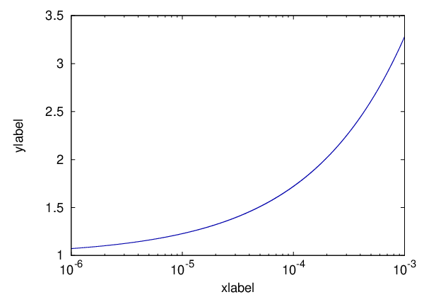
We see a clear connection between the neutrino–induced gravitational potential given by Eq. (20), , and the amplification of the peculiar velocity of matter. Even the values suggested by the observation of the bulk flow anomaly [4] can be reached.
Concerning the ISW, it would be desirable to also give an estimate that could be compared with the observed signal amplitude. Unfortunately, no robust estimation can be made at this stage. The background density oscillates with time [29] due to strong oscillations in the neutrino mass . If these oscillations visible in the background quantities also affect the non–linear neutrino lumps, the neutrino–induced gravitational potential will adopt this oscillatory behavior. Since its time derivative enters the ISW estimation (assuming a non–vanishing correlation between neutrino lumps and dark matter structures), every prediction would be extremely sensitive to small changes in the parameter values and to the details of the evolution. Moreover, since our discussion of the ISW in Sec. III is based on linear perturbation theory, it remains open whether a full non–linear treatment within growing neutrino quintessence would show new and different phenomena relevant for the ISW observable.
On the other hand, there is the realistic possibility, already mentioned above, that the neutrino–induced gravitational potential is sub–dominant. In this case, the evolution of the large–scale gravitational potential is dominated by matter and decays similarly to the CDM case. A neutrino lump in our cosmological vicinity could nonetheless generate a large local bulk motion. The neutrino fluid in growing neutrino quintessence is generically inhomogeneous on large scales allowing for local features that are unlikely in the standard scenario. The observed bulk flow could be such a phenomenon.
V Conclusion
In this work, we have investigated modifications to the standard cosmological model that could be required if the peculiar velocity anomaly persists. Extra couplings of the dark components are a natural possibility, as we have illustrated with two scenarios. We have also discussed the relationship between peculiar velocities and the ISW as observed in the cross–correlation between temperature fluctuations of the CMB and density fluctuations. Both are sensitive to the change of the gravitational potential with time in a similar range of length scales . While an enhanced bulk flow suggests a slower decrease of as compared to the fiducial CDM model, the observed ISW correlation requires an even faster decreasing . In models with more complex cosmological dynamics, this potential discrepancy can be alleviated by features in the time evolution of or if the large bulk flow is a local phenomenon.
As a first scenario, we have employed a coupling between dark energy and dark matter, which succeeds in generating large peculiar velocities but, in its simple form, conflicts with ISW observations. Our results suggest that more elaborate cosmological models with a dark coupling may be promising to resolve the peculiar velocity anomaly if, at the same time, they respect further constraints.
We have also considered the case in which the additional growth is not caused by an extra force directly acting on CDM particles, but rather indirectly via an extra gravitational potential. This feature is realized in growing neutrino quintessence, which includes a coupling between dark energy and neutrinos. Under the influence of this extra force, the neutrinos form large–scale structures in recent times, generating an additional gravitational potential felt by the matter perturbations. This scenario as well can be in accordance with the peculiar velocity measurements.
If the significance of the peculiar velocity anomaly will increase
with future observations, it will be a strong sign for physics beyond
the CDM concordance model. By our examples, we have seen that
modifications to CDM becoming effective only in the recent
epoch may be sufficient to generate large peculiar velocities. This
might suggest that the new physics is connected with the recent
transition to dark energy domination.
We thank Björn Malte Schäfer for interesting and useful discussions.
References
- [1] R. Watkins, H. A. Feldman, and M. J. Hudson, Mon. Not. Roy. Astron. Soc. 392, 743 (2009), eprint arXiv:0809.4041.
- [2] L. Perivolaropoulos (2008), eprint arXiv:0811.4684.
- [3] N. Afshordi, G. Geshnizjani, and J. Khoury, JCAP 0908, 030 (2009), eprint arXiv:0812.2244.
- [4] H. A. Feldman, R. Watkins, and M. J. Hudson, Mon. Not. Roy. Astron. Soc. 407, 2328 (2010), eprint arXiv:0911.5516.
- [5] Y.-S. Song, C. G. Sabiu, R. C. Nichol, and C. J. Miller, JCAP 1001, 025 (2010a), eprint arXiv:1001.1154.
- [6] E. Macaulay, H. A. Feldman, P. G. Ferreira, M. J. Hudson, and R. Watkins (2010), eprint arXiv:1010.2651.
- [7] J. Colin, R. Mohayaee, S. Sarkar, and A. Shafieloo (2010), eprint arXiv:1011.6292.
- [8] Y.-S. Song, C. G. Sabiu, I. Kayo, and R. C. Nichol (2010b), eprint arXiv:1006.4630.
- [9] S. J. Osborne, D. S. Y. Mak, S. E. Church, and E. Pierpaoli (2010), eprint arXiv:1011.2781.
- [10] D.-C. Dai, W. H. Kinney, and D. Stojkovic (2011), eprint arXiv:1102.0800.
- [11] A. Kashlinsky, F. Atrio-Barandela, D. Kocevski, and H. Ebeling, Astrophys. J. 686, L49 (2009), eprint arXiv:0809.3734.
- [12] A. Kashlinsky, F. Atrio-Barandela, H. Ebeling, A. Edge, and D. Kocevski, Astrophys. J. 712, L81 (2010a), eprint arXiv:0910.4958.
- [13] A. Kashlinsky, F. Atrio-Barandela, H. Ebeling, A. Edge, and D. Kocevski, Astrophys. J. 712, L81 (2010b), eprint arXiv:0910.4958.
- [14] A. Kashlinsky, F. Atrio-Barandela, and H. Ebeling (2010c), eprint arXiv:1012.3214.
- [15] F. Atrio-Barandela, A. Kashlinsky, H. Ebeling, D. Kocevski, and A. Edge, Astrophys. J. 719, 77 (2010), eprint arXiv:1001.1261.
- [16] L. Amendola, Phys. Rev. D60, 043501 (1999), eprint arXiv:astro-ph/9904120.
- [17] S. M. Carroll et al., Phys. Rev. D71, 063513 (2005), eprint arXiv:astro-ph/0410031.
- [18] A. A. Starobinsky, JETP Lett. 86, 157 (2007), eprint arXiv:0706.2041.
- [19] S. Carloni, P. K. S. Dunsby, and A. Troisi, Phys. Rev. D77, 024024 (2008), eprint arXiv:0707.0106.
- [20] S. Tsujikawa, Phys. Rev. D77, 023507 (2008), eprint arXiv:0709.1391.
- [21] Y. Gong, Phys. Rev. D78, 123010 (2008), eprint arXiv:0808.1316.
- [22] G. R. Dvali, G. Gabadadze, and M. Porrati, Phys. Lett. B485, 208 (2000), eprint arXiv:hep-th/0005016.
- [23] A. Cardoso, K. Koyama, S. S. Seahra, and F. P. Silva, Phys. Rev. D77, 083512 (2008), eprint arXiv:0711.2563.
- [24] J. Khoury and M. Wyman, Phys. Rev. D80, 064023 (2009), eprint arXiv:0903.1292.
- [25] C. Wetterich, Astron. Astrophys. 301, 321 (1995), eprint arXiv:hep-th/9408025.
- [26] L. Amendola, Phys. Rev. D62, 043511 (2000), eprint arXiv:astro-ph/9908023.
- [27] A. W. Brookfield, C. van de Bruck, D. F. Mota, and D. Tocchini-Valentini, Phys. Rev. Lett. 96, 061301 (2006), eprint arXiv:astro-ph/0503349.
- [28] L. Amendola, M. Baldi, and C. Wetterich, Phys. Rev. D78, 023015 (2008), eprint arXiv:0706.3064.
- [29] C. Wetterich, Phys. Lett. B655, 201 (2007), eprint arXiv:0706.4427.
- [30] K. Ichiki and Y.-Y. Keum (2008), eprint arXiv:0803.3142.
- [31] D. F. Mota, V. Pettorino, G. Robbers, and C. Wetterich, Phys. Lett. B663, 160 (2008), eprint arXiv:0802.1515.
- [32] G. Caldera-Cabral, R. Maartens, and B. M. Schaefer, JCAP 0907, 027 (2009), eprint arXiv:0905.0492.
- [33] M. B. Gavela, D. Hernandez, L. L. Honorez, O. Mena, and S. Rigolin, JCAP 0907, 034 (2009), eprint arXiv:0901.1611.
- [34] L. Mersini-Houghton and R. Holman, JCAP 0902, 006 (2009), eprint arXiv:0810.5388.
- [35] J. B. Jimenez and A. L. Maroto, JCAP 0903, 015 (2009), eprint arXiv:0811.3606.
- [36] S. Ho, C. Hirata, N. Padmanabhan, U. Seljak, and N. Bahcall, Phys. Rev. D78, 043519 (2008), eprint arXiv:0801.0642.
- [37] T. Giannantonio et al., Phys. Rev. D77, 123520 (2008), eprint arXiv:0801.4380.
- [38] E. V. Linder, Phys. Rev. D72, 043529 (2005), eprint arXiv:astro-ph/0507263.
- [39] E. V. Linder and R. N. Cahn, Astropart. Phys. 28, 481 (2007), eprint arXiv:astro-ph/0701317.
- [40] A. Hajian (2007), eprint arXiv:astro-ph/0702723.
- [41] C. J. Copi, D. Huterer, D. J. Schwarz, and G. D. Starkman, Mon. Not. Roy. Astron. Soc. 399, 295 (2009), eprint arXiv:0808.3767.
- [42] Y. Ayaita, M. Weber, and C. Wetterich, Phys. Rev. D81, 023507 (2010), eprint arXiv:0905.3324.
- [43] C. Wetterich, Nucl. Phys. B302, 668 (1988).
- [44] B. Ratra and P. J. E. Peebles, Phys. Rev. D37, 3406 (1988).
- [45] C. Wetterich, Phys. Rev. D77, 103505 (2008), eprint arXiv:0801.3208.
- [46] M. Doran, G. Robbers, and C. Wetterich, Phys. Rev. D75, 023003 (2007), eprint arXiv:astro-ph/0609814.
- [47] N. Brouzakis, N. Tetradis, and C. Wetterich, Phys. Lett. B665, 131 (2008), eprint arXiv:0711.2226.
- [48] A. E. Bernardini and O. Bertolami, Phys. Rev. D80, 123011 (2009), eprint arXiv:0909.1541.
- [49] N. Wintergerst, V. Pettorino, D. F. Mota, and C. Wetterich, Phys. Rev. D81, 063525 (2010), eprint arXiv:0910.4985.
- [50] V. Pettorino, N. Wintergerst, L. Amendola, and C. Wetterich, Phys. Rev. D82, 123001 (2010), eprint arXiv:1009.2461.
- [51] N. Nunes, L. Schrempp, and C. Wetterich (2011), eprint arXiv:1102.1664.