Exact-exchange kernel of time-dependent density functional theory: Frequency dependence and photoabsorption spectra of atoms
Abstract
In this work we have calculated excitation energies and photoionization cross sections of Be and Ne in the exact-exchange (EXX) approximation of time-dependent density functional theory (TDDFT). The main focus has been on the frequency dependence of the EXX kernel and on how it affects the spectrum as compared to the corresponding adiabatic approximation. We show that for some discrete excitation energies the frequency dependence is essential to reproduce the results of time-dependent Hartree-Fock theory. Unfortunately, we have found that the EXX approximation breaks down completely at higher energies, producing a response function with the wrong analytic structure and making inner-shell excitations disappear from the calculated spectra. We have traced this failure to the existence of vanishing eigenvalues of the Kohn-Sham non-interacting response function. Based on the adiabatic TDDFT formalism we propose a new way of deriving the Fano parameters of autoionizing resonances.
pacs
31.15.Ew, 31.25.-v, 71.15.-mI Introduction
The photoabsorption spectrum of an atom or molecule reveals detailed information about the structure and dynamics of its constituent electrons. Important phenomena, such as Fano resonances[1] and multiple-particle excitations, which can solely be attributed to the electron- electron interaction, has been under extensive experimental and theoretical investigation for several decades. To describe and quantify these exciting many-body effects is, however, still a major theoretical challenge. Traditional approaches to this problem are based on infinite-order many-body perturbation expansions which lead to complicated integral equations already at the Hartree-Fock level of approximation. This level of approximation is also referred to as the random phase approximation with exchange (RPAE) and was extensively used by Amusia[2, 3] and by Wendin[4] for the description of atomic photoabsorption spectra. From a mathematical or numerical point of view this entails the solution of an integral equation known as the Bethe-Salpeter equation for a four-point vertex function, the solution of which is computationally very demanding in low-symmetry systems like larger molecules or nano structures.
Since the pioneering work of Ando[5] and Zangvill and Soven[6] in the late seventies, time-dependent density functional theory[7, 8] (TDDFT) has emerged as a more convenient route toward the calculation of spectral properties. Within TDDFT, as it is presently formulated, only two-point correlation functions appear and, in addition, one arrives at explicit expressions for the linear density response function, thus avoiding the need for integral equations. The price to pay is the difficulties associated with obtaining approximations to the frequency-dependent exchange-correlation (XC) kernel, constituting one of the basic elements of TDDFT. In most calculations until today one uses a static, frequency-independent, kernel. These so called adiabatic approximations have, in many cases, produced relatively accurate and important results - especially for static properties or small excitation energies. There are, however, many cases where the inadequacies of the adiabatic approximations are easily discernible.
Until recently, no systematic way of obtaining successively better approximations to the XC kernel of TDDFT has been available. By means of the variational formulation of many-body theory[9] we have recently developed a tool for constructing approximations to the XC kernel, which not only incorporates the important energy dependence of the kernel but does it in a way so as to guarantee the fulfillment of many sum rules and conservation laws.[10] As discussed in these previous publications the variational approach is not uniquely defined and some implementations are preferable to others. For instance, starting from the functional of Luttinger and Ward[11] (LW) is usually a better approach as compared to starting from the Klein functional.[12] The simplest approximate kernel derived from the latter functional is that of the time-dependent exact-exchange (TDEXX) approximation. This approximation can be considered as an attempt to mimic the time-dependent Hartree-Fock approximation within a TDDFT framework, a point which has been discussed at length in previous work.[13, 14] The exact-exchange (EXX) kernel has, however, yet received little attention especially with regard to its ability to describe spectral properties which necessitates a calculation on the real frequency axis. Previous investigations have either addressed the adiabatic limit,[15, 16] focused on extended systems at low frequencies[17] or most recently carried out model calculations in the time domain.[18]
The present paper presents a numerical and analytical investigation of the fully frequency-dependent EXX kernel of closed-shell atoms. It is the fourth and latest in a series of papers by us concerned with approximations obtained from the variational scheme to TDDFT. In the first paper[13] we calculated the EXX kernel of the electron gas. From that kernel we obtained the interacting density response function of the gas, a quantity which enabled us to calculate the correlation energy via an integration over the strength of the Coulomb interaction. The results turned out to be rather close to accurate Monte-Carlo results. From the response function one can also indirectly obtain a local vertex function which can be used to calculate the electron self-energy and thus the one-electron Green function. Unfortunately, this local vertex turned out to be too simple minded to remedy the infamous band-narrowing problem[19, 20] in simpler metals - and in transition metals for that matter.[21] In the second paper[22] we went beyond the EXX approximation and calculated the XC potential at the level of the self-consistent GW approximation in atoms. This potential turned out to be superior to that of the second-order Møller-Plesset (MP2) approximation,[23] at least in the outskirts of the atoms. The resulting ionization potentials turned out to be surprisingly accurate. In the third paper[14] we calculated the EXX kernel at imaginary frequencies and used it to calculate static polarizabilities, van der-Waals coefficient and correlation energies of closed-shell atoms. The polarizabilities and van der-Waals coefficients were very similar to those of time-dependent Hartree-Fock theory and thus not very accurate. (See also Ref. 24.) On the other hand, we obtained better than 95% of the correlation energies which should be compared to errors of the order of a factor of two within the RPA. In contrast, our calculated discrete particle-conserving excitation energies were not far from those of the RPA. We attributed this partial failure to a poor description of the ground state within the EXX approximation.
It is interesting to investigate the performance of the TDEXX approximation as far as concerns the description of photoabsorption spectra. In previous papers we were, relying on a new numerical technique based on cubic splines. While this technique turned out to be ideally suited for the necessary inversion of the non-interacting density response function and also for the calculation of discrete excitation energies, the method was less effective in the case of continuous spectra. This deficiency is mainly a result of a too sparse and unpredictable sampling of the continuum especially at larger energies, something which would require a prohibitively large number of splines to remedy. For these reasons we have in the present work designed interpolation schemes and new numerical methods for directly extracting the important parameters determining the shape of the Fano resonances[1] resulting from the existence of quasi discrete inner-shell levels interacting with continua.
While we have seen that the energy dependence of the EXX kernel can improve on many of the deficiencies of typical adiabatic (read static) approximations we have in the present work made a very important although somewhat disappointing discovery. The TDEXX completely fails to describe parts of the spectra, especially at higher energies. At least if the spectra are calculated from Fourier transforms to frequency space as most researches consider to be the most natural approach.[25] Moreover, this failure is not connected, e.g., to the neglect of processes describing correlation effects. The failure is caused by the existence of zero eigenvalues of the non-interacting response function at certain energies. Any method for constructing an XC kernel starting from the linearized Sham-Schlüter (LSS) equation will suffer from the same ailment no matter how much of correlation one is trying to account for. And those variational approaches to many-body theory which build on the Klein functional will always result in the LSS equation, suggesting that a reasonable theory for constructing better kernels should start from a more elaborate variational functional like, e.g., that due to Luttinger and Ward. But this is, of course, only speculation at the present stage. Such investigations will be the topics of future works.
The paper is organized as follows. In Sec. II we present the linear response matrix equation for excitation energies and oscillator strengths and discuss how a frequency-dependent kernel might influence the results. In Sec. III we present the EXX equations. We also discuss possible generalizations and point out inherent limitations and potential problems. In Sec. IV the numerical method is briefly discussed. Sec. V is devoted to numerical results with a presentation of the EXX kernel and the consequences of zero eigenvalues in the KS response function. The excitation energies and continuum spectra of Be and Ne are also presented and compared to the results of the RPA and the adiabatic EXX (AEXX) approximations. In Sec. VI we give our conclusion and summarize our findings and, finally, in the Appendix we derive the Fano-profile formula[1] using the adiabatic TDDFT formalism.
II Linear response equation
Within TDDFT the electronic linear density response function is given by
| (1) |
where is the Kohn-Sham (KS) linear density response function, is the Coulomb interaction and is the XC kernel defined as the functional derivative of the XC potential ,
| (2) |
Eq. (1) can be considered as a matrix equation in and or in any other suitable basis.
The KS linear density response function or, equivalently, the retarded KS polarization propagator, can be written as
| (3) |
Here, is a composite index, in which labels an occupied state and an unoccupied state. The excitation function is a product of an occupied and an unoccupied KS orbital and is a KS excitation energy. The tilde in signifies a multiplication by . With in this representation, Eq. (1) for the full can be rewritten as[26]
| (4) |
where is the identity matrix and
| (5) |
The second term represents an integral over all spatial variables of multiplied with two excitation functions and . The matrix is symmetric and if, in addition, is frequency-independent and hence real, can be diagonalized as , where is a diagonal matrix. Then Eq. (4) simplifies to
| (6) |
Here, , where is the unitary matrix which diagonalizes . The square root of the eigenvalues can be interpreted as the new transition frequencies and as the excitation amplitudes.[27] For most known, or generally used, adiabatic kernels the matrix is dominated by the Coulomb interaction and therefore its eigenvalues are positive. As a consequence has the correct analytic structure with a positive spectral function. It is also easy to see that both and have the same large frequency behavior and thus both obey the -sum rule.
A frequency-dependent with the correct analytic structure requires to have both real and imaginary parts. The matrix is then not Hermitian. It is, however, still symmetric and can, in general, be diagonalized according to , where the eigenvalues and eigenvectors now can be both complex and -dependent. A particular consequence of having a frequency-dependent kernel is that more zeros in the denominator of Eq. (6) can be generated, which would imply more resonances in . These resonances could correspond to multiple-particle excitations or other excitations of collective nature. Unfortunately, an approximate frequency dependence is not guaranteed to yield a positive spectral function. It could also lead to poles in the upper half of the complex plane, thus destroying the analytic structure of . We will later demonstrate that this is indeed a reality to be considered.
III Exact-exchange equations
The derivation of the EXX potential and kernel has been given in several previous publications by us[10, 22, 14] and others.[28, 16] Our choice of approach is to start from that variational approach to many-body theory which builds on the Klein functional.[12] This functional of the Green function gives us the total action of the system and it contains the functional whose derivative with respect to the Green function gives the electronic self energy, .[29] When possible Green functions are restricted to those which can be generated by local multiplicative potentials the action becomes a functional of the density. The stationary property of the action with respect to variations in the particle density yields the linearized Sham-Schlüter (LSS) equation[30] for the KS potential (with ):
| (7) |
where is the self-energy calculated with KS orbitals generated by and
Here, is the KS Green function and is the total effective potential of the KS system. A further variation of the LSS equation with respect to the potential results in an equation for :
| (8) |
where .
In the EXX approximation one chooses the HF approximation for the functional ,
| (9) |
and the variation of the resulting self energy with respect to becomes
The terms on the right hand side of Eq. (8) are, in this approximation, represented diagrammatically in Fig. 1.

The first order vertex diagram, the first on the second row in Fig. 1), which will be referred to as , is given in terms of KS orbitals and eigenvalues as
| (10a) | |||
| where and is the occupation number of state . The other four diagrams are self-energy terms and their sum, referred to as , is: | |||
| (10b) | |||
We see immediately that the poles of and are located at the KS eigenvalue differences, just as in the case of . The EXX approximation can, therefore, not describe multiple-particle excitations. In order to incorporate those one has to include diagrams which contain new poles, as obtained, e.g., by choosing in the GW approximation. The new poles are in that approximation generated by the dynamically screened interaction, .
It is apparent from Eq. (1) that only the quantity is needed to obtain the spectrum. Consequently, it is sufficient to invert once in Eq. (8). It has, however, been known for some time that is not always invertible due to the existence of nontrivial vanishing eigenvalues at particular frequencies.[31] At these frequencies there exists an external perturbation which does not produce a density response to first order. Thus, in the unlikely case that has zero eigenvalues at the same frequencies the kernel diverges.[32] This can have a drastic effect on the calculated spectra as we will see later.
IV Numerical approach
For the numerical implementation we have used an approach based on cubic splines as radial basis functions. This approach was used also in previous works[22, 14] and showed to be ideally suited for solving equations where an inversion of is needed. In short, a cubic spline is a piecewise third order polynomial with compact support. Defined on four sub-intervals, and hence composed of four different third order polynomials with in total 16 unknown constants, it is uniquely determined up to a multiplicative constant by imposing continuity up to the second derivative. A mesh is distributed on the -axis up to a finite and the basis set is formed by constructing a spline starting at every mesh point and extending over four intervals. In this way the splines only overlap with its three nearest neighbors on either side. The basis set is complete on the interval in the limit , where is the number of splines. A review on the use of general B-splines in electronic structure calculations can be found in Ref. 33.
The numerical solution of Eqs. (7-8) involves the calculation of products of KS orbitals. The completeness of the spline basis allows us to re-expand these products in splines, thus casting the original problem into a linear system of equations. The accuracy of this procedure was checked by increasing the number of splines and a fast convergence was observed.
For the discrete part of the spectrum in the TDEXX approximation we have extracted both excitation energies and oscillator strengths from the position and the hight of the peaks of . In the RPA and the AEXX the kernels are frequency independent and thus excitation energies and oscillator strengths can be directly obtained from the eigenvalues and eigenvectors of matrix , defined in Eq. (5). We will now describe the method that we used in the continuos part of the spectrum.
Once the radius is fixed the system studied is actually an atom in a box. It turns out, however, that the discrete positive energy states provide a good description of the true continuum orbitals at the same energy but with a different normalization. To get the correct normalization the box states only need to be multiplied with a local density of states factor. By choosing an appropriate mesh both bound and continuum orbitals are well described within the same basis.

In our calculation we have used a mesh which starts as cubic and then smoothly changes to a linear mesh, according to the formula
| (11) |
The photoionization cross sections have been obtained by first interpolating the discretized up to large energies, which is possible since it is a smooth function of for every and . The real part of was then obtained through the Kramers-Kronig relations. This was done for every continuum channel. Since the bound states are not coupled to the continuum in the KS system, the discrete part of can simply be added to form the total non-interacting response function of the atom. The resulting response function is then used to solve Eq. (1) and to obtain the interacting continuum. The accuracy of this method has been checked by calculating the RPA spectra of some atoms and comparing them with those of other works.[34, 35]
V Results and Discussion
In this section we present numerical results on the EXX kernel for the Be and Ne atoms. The photoabsorption spectra calculated using this kernel as well as its adiabatic counterpart are presented and compared. We begin with a study of the vanishing eigenvalues of the KS linear density response function . This analysis will be useful to interpret and understand the structure of the EXX kernel in the frequency domain.
V.1 Vanishing eigenvalues of
Mearns and Kohn,[31] showed that can have nontrivial vanishing eigenvalues for finite systems at certain frequencies. Physically this means that there is a monochromatic perturbation which differs from a constant, and which yields a vanishing density response. Note that this is true only if the perturbation is not switched on at a particular time. If that is the case there is always a finite density response.[36]
The condition for having a vanishing density response , at frequency , can be expressed as
| (12) |
where is an eigenvector of corresponding to an eigenvalue equal to zero and describes the spatial part of the monochromatic perturbation. With only one occupied orbital like, e.g., in He, the -functions are linearly independent. In that case vanishes only if the integral in is zero for every , a condition which implies to be independent of position. On the other hand, with more than one occupied level the -functions are linearly dependent and hence it is, in general, possible to find a , different from a constant, that fulfills Eq. (12).
The Be atom has two occupied levels and is therefore the simplest closed-shell spin compensated atom for which a nontrivial zero eigenvalue can occur. We have diagonalized (in the EXX approximation) for the excitation channel of the Be atom in a large finite box (40 a.u.) and found a number of eigenvalues which pass through zero. The first zero can be found around 2 a.u., an energy far above the first ionization threshold. At higher frequencies, a set of zeros are found close to the excitation energies of the inner -shell. The eigenvalues of for frequencies in the range of the and transitions are displayed in Fig. 2. We note that close to the transition (3.948 a.u.) there is an eigenvalue which crosses zero at 4.005 a.u., and that close to the transition (4.058 a.u.) a second eigenvalue crosses zero at 4.072 a.u.. We have in fact observed that there is one vanishing eigenvalue close to every inner-shell transition.
The Ne atom has three occupied shells and, therefore, a larger number of vanishing eigenvalues are expected. Indeed, vanishing eigenvalues where found already at low frequencies before the first ionization threshold. We did, however, not find any vanishing eigenvalues before the first excitation energy, in agreement with the findings in Ref. 31.
For the numerical calculations of the eigenvalues the atom has been confined to a finite box, albeit large. The response function is then a sum of discrete transitions and it is real almost everywhere. In the limit of an infinite box acquires a finite imaginary part at frequencies in the continuum. The zero eigenvalues may then also acquire a finite imaginary part.
As seen from Fig. 2 the eigenvalue of which passes through zero is proportional to for frequencies close to . The inverse of will, therefore, diverge as a simple pole. If the sum in Eq. (10) has a finite component along the eigenvector with zero eigenvalue it may have severe consequences for the calculation of , as we will see shortly.
A natural way of handling problems associated with zero eigenvalues of matrices which need to be inverted is so called singular value decomposition. This means that one finds the eigenvector corresponding to the zero eigenvalue and then invert the matrix in the subspace orthogonal to that eigenvector. Notice, however, that eigenvalues of are frequency dependent and projecting out states within a limited range of frequencies will result in abrupt changes in the spectrum at the borders of the frequency range. And we can find no physical motivation for such drastic manual changes.

V.2 The EXX kernel

As noted previously,[37, 14] the XC kernel is not uniquely defined by Eq. (8). Given an one can always add two arbitrary functions and without changing the results for . This originates in the fact that the potential is determined up to the addition of a purely time-dependent function and that the density variations must integrate to zero. When we discuss and its dependence on the frequency we instead consider the quantities , which are unique since the excitation functions integrate to zero and thus remove the effect of adding functions of the form and .
Let us first consider the case of the He atom, or for that matter, any other spin-compensated two-electron system. In this case equals minus half the Coulomb potential . This can be seen either by noting that the EXX potential becomes and hence the functional derivative can be taken explicitly, or after some manipulations of the diagrammatic expression in Eq. (10). In the latter case it is important to impose the LSS equation as well as the additional constraint[38]
where denotes the highest occupied orbital. We thus see that for He the EXX kernel is energy independent.
Let us now consider systems with more than one occupied orbital. The Be atom has two filled closed shells - the inner 1s-shell and the outer 2s-shell - and a full numerical solution is therefore required. The kernel for the channel was calculated with a finite box radius of 40 a.u.. At low frequencies has a weak frequency dependence and is purely real. At larger frequencies, however, develops a strong frequency dependence and around 2 a.u. the kernel diverges. In Fig. 3 we show the real and imaginary parts of around this point. The divergence is typical of a double pole with the real part given by the difference between a term and a squared delta function, . A small asymmetry around the pole can be observed which indicates the presence of an additional simple pole. The exact location of the pole can be traced back to the first vanishing eigenvalue of (see discussion in the previous section). The pole structure of shows that does not compensate for the zero of .


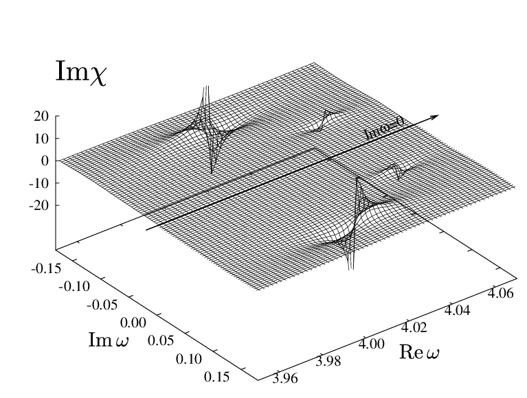
Continuing to higher frequencies more singularities in the kernel are observed. Near the transition in a second pole in develops. As a matter of fact we find a pole in close to every transition in (see the upper panel of Fig. 4). These poles have the same structure as the one at 2 a.u. and are also confirmed to originate from the vanishing eigenvalues of . The vanishing eigenvalues corresponding to the first two inner-shell excitations are displayed in Fig. 2. The double and simple pole structure in is expected since, in order to calculate the kernel, has to be inverted twice, see Eq. (8). Let us call the eigenvector of with eigenvalue . Then from the equation the kernel can be expressed as
| (13) |
If we denote by the frequency for which there is an eigenvalue equal to zero, we have that for and Eq. (13) can be cast in a more transparent form
| (14) |
where the quantities , and are weakly dependent on , and the and dependence has been suppressed. Notice that the object , the basic quantity needed to calculate the full response function , only has simple poles at the same frequencies.
The kernel for the Ne atom has an even larger number of poles due to the larger number of inner-shells and thus a larger number of vanishing eigenvalues of its . All poles are of the same structure as those discussed for Be, but the first pole appears already between the first and second resonance in , i.e., below the ionization threshold of Ne.
As can be seen from Eq. (13) the -representation is not well suited for studying the singular behavior of the kernel in real space. The elements of the matrix in Eq. (5) will all have the pole structure described above. When the matrix is diagonalized, however, this pole structure survives in only one of the eigenvalues, whereas the remaining ones appear to have a smooth frequency dependence but still affected by the pole giving rise to an oscillatory behavior. In Figs. 4 and 5 two different smooth eigenvalues of this matrix are shown for Be and Ne respectively. The eigenvalue corresponding to the transition in Be is weakly dependent on the frequency and hence the intersection with the line giving the location of the new excitation energy is only slightly shifted from that of the adiabatic approximation. The new position in the TDEXX approximation is in better agreement with the corresponding excitation energy of the TDHF approximation as compared to the same position in the adiabatic case, see Tab. 1. The position of the first discrete excitation in Ne is, however, strongly modified by the frequency dependence as is shown in Fig. 5. The kernel of the adiabatic approximation moves the peak to a lower frequency as compared to the RPA while the TDHF result lies at a higher frequency (0.674 a.u.). The frequency dependence of the kernel leads to the opposite effect and moves the peak even a little beyond the true TDHF value. At a somewhat larger frequency the EXX kernel has a pole and the eigenvalue corresponding to the excitation is seen to oscillate (see lower panel of Fig. 5). The maximum of the oscillation occurs exactly at the location of the pole. Apart from the desired solution, i.e., the crossing with the -line at 0.680 a.u., there are two more crossings. The first of these corresponds to the small negative peak found in the spectrum (at 0.71 a.u.) and the next has zero oscillator strength. Clearly, the negative peak is unphysical but we expect that the ability of the TDEXX to describe the spectrum rapidly decreases as we approach the pole.
Since there is a pole close to every inner-shell excitation the eigenvalues oscillate in these regions. The eigenvalue corresponding to an inner-shell excitation gives only one solution exactly at the pole as seen in the upper panels of Figs. 4 and 5. This is true for all inner-shell transitions in Be and Ne and seems to be a general behavior. The oscillator strength is zero at these points leading to a complete disappearance of the peaks from the spectrum as also seen, e.g., at third crossing corresponding to the first excitation in Ne as discussed above. Because the sum rule is obeyed the missing oscillator strength is expected to be transferred to excitations of the outer shell. This conjecture is based on having the correct analytic structure of the response function with a Lehmann representation leading to the fact that the large frequency behavior of the response is determined by the sum of the different oscillator strengths. Unfortunately, in many cases the three solutions at the real frequency axis close to the double pole structure, which we discussed above, instead leads to one solution at the real axis and two more complex solutions one of which is in the upper half plane and the other in the lower.
| Trans. | KS(EXX) | RPA | AEXX | TDEXX | TDHF11 1 From Ref. 39 and 40 | KS(Exact)22 2 From Ref. 41 | Exp.44 4 From Ref. 42 |
|---|---|---|---|---|---|---|---|
| Be | |||||||
| 1s2p | 3.948 | 3.959 | 3.956 | 4.00533 3 Transition calculated assuming no inter-shell coupling. | 4.346 | 4.017 | 4.243 |
| 1s3p | 4.058 | 4.060 | 4.059 | 4.07233 3 Transition calculated assuming no inter-shell coupling. | 4.646 | 4.153 | 4.461 |
| 2s2p | 0.131 | 0.203 | 0.177 | 0.176 | 0.176 | 0.133 | 0.194 |
| 2s3p | 0.241 | 0.255 | 0.247 | 0.247 | 0.247 | 0.269 | 0.274 |
| Ne | |||||||
| 2s3p | 1.604 | 1.608 | 1.607 | 1.60933 3 Transition calculated assuming no inter-shell coupling. | - | 1.542 | 1.674 |
| 2s4p | 1.667 | 1.668 | 1.667 | 1.66933 3 Transition calculated assuming no inter-shell coupling. | - | 1.602 | 1.731 |
| 2p3s | 0.659 | 0.667 | 0.663 | 0.680 | 0.674 | 0.612 | 0.619 |
| 2p4s | 0.779 | 0.781 | 0.780 | 0.783 | 0.782 | 0.725 | 0.727 |
Thus the proper analytic structure of the response is destroyed and the fact that the TDEXX response has the correct large frequency behavior does not guarantee that the full spectrum contains the correct sum of oscillator strengths. Part of the spectrum is actually missing which is a clear failure of the theory. In Fig. 4 clearly exhibits two peaks located symmetrically on opposite sides of the real axis. Apart from the solution with zero oscillator strength there are thus two more solutions at complex frequencies ().
Finally, before further discussing the spectrum we will make a small digression and investigate the eigenvalues of . In Fig. 2 the eigenvalues of both and are presented in a frequency range where there are two vanishing eigenvalues of . We see, however, that also have vanishing eigenvalues at the same points. We also see that the eigenvalues of only touches the zero intensity axis whereas the eigenvalues of cross this axis. This can be explained by studying
| (15) |
obtained by using the equation . Our calculations show that the matrix does not have a zero eigenvalue where has. Consequently, by writing this equation in the basis of the eigenvectors of , we immediately see that behaves as close to . There is no reason to believe that the Coulomb interaction would change the simple zeros of to double zeros. We therefore expect also to have simple zeros although shifted relative to those of . From the definition of the exact XC kernel,
| (16) |
should have simple poles where and have vanishing eigenvalues. The double pole structure found within the EXX approximation is thus an artifact of this theory.
V.3 Discrete excitation energies
Before the first ionization threshold the atomic photoabsorption spectra consists of a set of discrete transitions. In Tab. 1 the first two discrete transitions are presented for Be and Ne. A comparison is made between the AEXX, TDEXX, TDHF and the RPA as well as the KS eigenvalue differences of the exact[41] and the EXX potentials. The latter potential was also used when calculating in the aforementioned approximations.
The TDEXX approximation is expected to give results close to TDHF. In this sense the outer-shell transitions of Be are well described already in the AEXX approximation. By also accounting for the frequency dependence the results improve even further. For the outer-shell excitations of Ne dynamic effects in are crucial. The AEXX approximation reduces the values of the RPA whereas the TDHF results are larger than those of the RPA. The frequency dependence corrects this tendency yielding results in good agreement with TDHF, although somewhat over-estimated. The effect of the kernel on the first excitation energy of Ne is illustrated in Fig. 5. The results of TDHF and hence of TDEXX differ markedly from the experimental values. By looking at the exact KS eigenvalue differences it can be concluded that the error is mainly related to the effect of the ground state potential. The kernel has only a small effect on the outer shell excitation energies as was previously pointed out by Petersilka et. al..[43]


A description of inner-shell excitation energies in terms of density functional eigenvalues is bound to fail. In Tab. 1 we see that the true core excitation energies are largely under-estimated by even the exact KS eigenvalue differences as compared to the true excitation energies. An adiabatic kernel is unable to correct these errors as confirmed by the examples (RPA and AEXX) shown in the table. A strong frequency dependence in the kernel might, however, improve the situation considerably. The vanishing eigenvalues of result in a strong frequency dependence in the EXX kernel near these excitations. As we saw in Sec. IIIC this frequency dependence is, however, too strong and even produces the wrong analytic structure of the response. The matrix contains separate diagonal blocks for different excitation channels and off diagonal blocks for the coupling between them. Notice, however, that this separation is not entirely well defined since part of the inter-channel coupling is already contained in . By including and diagonalizing only the block containing the inner-shell excitations we obtain some improvement for the position of these. Accordingly, for Be we have diagonalized the block and for Ne we have diagonalized the block. The results are marked in Tab. 1. The most important observation here is the fact that by means of this somewhat ad-hoc procedure we can obtain results for those inner-shell excitations which completely vanish in the full treatment.
The calculation of the inner-shell transitions was done with a finite box size and the excitation energies where extracted from the location of the delta peaks in . In reality these peaks will be somewhat shifted and broadened forming a so-called Fano resonance due to the coupling to continuum channels. In the next section we will present results for these resonance structures.
V.4 Photoionization cross sections and
Fano resonances
The photoionization cross section of Be is presented in Fig. 6 and different approximations are compared. The experimental result has not been included since in this region the spectrum is dominated by the and double excitation resonances, which cannot be captured by the approximations studied here. The figure shows that the AEXX and the TDEXX approximations are almost indistinguishable and also very close to the RPAE results of Amusia et. al.[44] We remind the reader that the RPAE approximation is identical to linearized TDHF. The frequency dependence of the kernel is weak up to around 2 a.u. where the first singularity of occurs. This strong frequency dependence of has, however, only a small effect on the spectrum in the studied region.
The photoionization cross section after the first ionization threshold of Ne is presented in Fig. 7. It contains two ionization channels, to continuum or . The AEXX agrees very well with the RPAE results.[45] There is also a fairly good agreement with experiment.[46] In the figure we have deliberately not presented results obtained by including the full energy dependence of . In the energy region covered by Fig. 7 the non-interacting response function of Ne has a number of zero eigenvalues producing violent structures in . This unphysical behavior results in a series of strong peaks also in the full response. Thus including the energy dependence of results in absorption spectra with no resemblance to the spectra in Fig. 7. These strong structures are of course obtained using discrete splines which give only a discrete sampling of the continuum. It could be possible that calculating using true continuum functions would somehow alleviate this problem even though it will not go away completely. The zero eigenvalue below the ionization threshold does produce unphysical structure in the absorption spectra of Ne. In this case one cannot blame the unphysical spectrum on the lack of a proper continuum, and we are convinced of the futility in going through the trouble of calculating proper continuum functions.


At higher frequencies, Fano resonances due to excitations of inner-shell electrons occur. In the Appendix we present a derivation of the Fano profile formula for excitations with single-particle character starting from the linear density response function within adiabatic TDDFT. The Fano parameters , , and are there given expressions in terms of the adiabatic kernel , see Eq. (23) and Eq. (27). In Figs. 6 and 7 we compare spectra calculated either directly from Eq. (1) using an interpolated or by employing the analytic method described in the Appendix. Within the analytic approach we have for both Be and Ne ignored the coupling between different discrete states via the continuum (which corresponds to ignoring the off-diagonal elements of the matrix in Eq. (28)). For Ne we have also assumed that we can ignore the coupling between the and continua, which can be reached from the -shell. The Figs. 6 and 7 contain results of both the RPA and the AEXX approximation. As seen, the two different ways of calculating the spectra around a resonance give almost identical results. This verifies the validity of the assumptions made above.
The two first inner-shell resonances of Be are very sharp with a zero on one side of the resonance due to the coupling to only one continuum. The very large -parameter is accompanied with a very small width, and meV in the RPA and and meV in the AEXX approximation, for the case of the resonance. In Ref. 47 the same parameters were calculated using the ALDA kernel giving similar results for the -parameter. The width () from the AEXX approximation is, however, a factor of two smaller than those from both the RPA and the ALDA. Experimental results have in this case not been found.
In Ne the discrete excitations of the -shell couples to both the and the continua. The minima on one side of the resonances therefore never reaches zero, which means that . This parameter is for the first resonance in the RPA and in the AEXX approximation. Since the experimental value is the AEXX approximation improves over the RPA. The widths are meV in the RPA and meV in the AEXX approximation. Again, the value of the AEXX approximation is in quite good agreement with the experimental result of 13 meV. The parameter differs, however, substantially from the experimental values. The RPA gives 6.3 and the AEXX approximation 3.5 whereas the experimental value is 1.6. In Fig. 7 the two first resonances of Ne are displayed. We clearly see that the shape is very sensitive to the -parameter. Notice that the experimental[48] and the RPAE results of Amusia[3] are shifted in order to facilitate the comparisons. The RPAE approximation yields and meV. The latter is about three times larger than the experimental value. In conclusion we can say that for the resonance of Ne neither of the static approximations here give a reasonable account of the experimental findings. The deviations to experiment is in many cases much larger than the results from different theories. A more sophisticated theory is therefore required. Theories which do provide a reasonable description of the spectra are wave function based, include many terms in a configuration interaction expansion, and can hardly be used on larger systems.
VI Summary and conclusions
In the present work we have used the so called exact-exchange approximation within TDDFT to calculate particle conserving discrete excitation energies and photoabsorption spectra of a few spherical atoms. As in several earlier papers on this topic we have also here relied on a numerical method based on cubic splines as basis functions for one-electron wave functions, polarizabilities, and the XC kernel. Clearly, such a numerical method amounts to a discretization of the continuum in which we have no control over the resulting positions of one-electron eigenvalues or electron-hole excitation energies which are ingredients in the necessary correlation functions. In order to circumvent such problems we have here constructed interpolation schemes which work very well for the description of, e.g., the non-interacting KS response function and other functions in the continuous part of the spectrum. In addition, we present in the Appendix a new way in which the parameters of the Fano profiles associated with the autoionizing resonances corresponding to inner-shell excitations can be calculated directly within adiabatic TDDFT without resorting to a full calculation of the entire spectrum. The resulting parameterized spectra are actually very accurate approximations to the full spectra which was demonstrated for the RPA and for the spatially non-local EXX kernel evaluated at zero frequency (AEXX). But, unfortunately, it has not been true when we have tried to incorporate the full frequency dependence of the EXX kernel. For reasons which have been discussed in the paper and will be mentioned again later on, the violence of that frequency dependence has defied any reasonable interpolation scheme. As a result we present few results based on the fully frequency dependent EXX kernel.
One such result is the calculation of discrete transition energies. There are really no strong trends in the results. We here compare our results to the corresponding results from a full time-dependent Hartree-Fock (HF) calculation. As discussed in the paper, this is motivated by our belief that the latter calculation is the ’target’ for the TDEXX approximation. It is not motivated by the HF results being very close to experiment which they are not. We find that the rather poor eigenvalue differences in the EXX approximation are improved by the inclusion of the Hartree part of the kernel (the RPA results). Then, for Ne, the situation deteriorates when the static (adiabatic) exchange effects are included just to again improve when the exchange effect are treated in a frequency dependent fashion. The full frequency-dependent kernel has, however, a tendency to overcorrect the errors from the RPA. In the case of Be the results of the adiabatic approximation instead represent a marked improvement on the RPA results and the frequency dependence gives a slight additional improvement. In all fairness we must add that these feeble trends are completely overshadowed by starting from a better XC potential like the exact DF potential available for the light atoms or from the very similar XC potential from a full GW calculation. The outer transition energies then move much closer to experimental results.
In the continuous part of the spectra we have used our new way of obtaining the parameters of the Fano line shapes and compared our results to those of the RPA, to previous calculations using different versions of the ALDA, and to experiment. We have found that all adiabatic kernels including the AEXX give a clear improvement over the RPA results for those Fano parameters which, roughly, correspond to the weights and the widths of the resonances with a slight edge for the AEXX approximation. The fact that the parameter mainly responsible for the height of the resonances is poorly described by all static approximations suggests that the former results are fortuitous. This impression is further reenforced by observing that a supposedly superior treatment including full energy dependence like the RPAE yields results for the parameters which are further away from experiment. Turning then to the density-functional version of RPAE, i.e., the TDEXX the description completely breaks down and the resonances disappear as will now be discussed.
Perhaps the most important finding of the present work is the violent frequency variation of the EXX kernel discovered in the vicinity of energies associated with inner-shell excitations. This, in turn, is a result of vanishing eigenvalues of the non-interacting Kohn-Sham response function close to these energies, and the necessity to invert that response function in order to obtain the resulting EXX kernel - at least in the way we presently formulate the theory. Although we can observe a tendency of the EXX kernel to use a strong frequency variation as a way to mimic the effect of the non-local but frequency independent three-point vertex of time-dependent Hartree-Fock theory this frequency behavior is quite unphysical and actually leads to the complete disappearance from the spectrum of all inner-shell excitations. We here trace this breakdown of the TDEXX approximation to the appearance of poles at a finite distance in frequency into the upper complex frequency plane thus producing a density response function with an incorrect analytic structure. One might think that this could be an order of limits issue and that the problem might go away if a proper continuum was included in the calculations. We doubt the correctness of this conjecture because the problem is already visible in the truly discrete part of, e.g., the Ne spectrum. In the present approach we implicitly calculate the linear response to a perturbation which has a sinusoidal variation at all times. It has been shown by van Leeuwen[36] that the non-interacting response function is always invertible for perturbations which completely vanish before a given time. This suggests that a proper TDEXX spectrum could be obtained by applying a sinusoidal perturbation at one particular time, propagate the time-dependent EXX orbitals, wait a time T until all transients have died out and then Fourier transform the charge density starting from time T to a very large time. This would amount to some limiting procedure which is quite feasible to carry out. It is, however, hard to see that such an approach would lead to something different to what we already have obtained.
It should be noted that the inclusion of higher-order correlation effects like, e.g., screening or relaxation effects will not be a remedy to the problem. Any procedure for obtaining better XC kernels based on the variational formulation of many-body theory and the Klein functional will lead to the linearized Sham-Schlüter equation at the first variation, albeit with a very sophisticated self-energy containing many physically important correlation effects. One further variation of the LSS equation in order to obtain the kernel will again reveal the necessity to invert the non-interacting Kohn-Sham response and the problem is still there. Only by pure coincidence will the right hand side of the equation determining the kernel have a zero eigenvalue at the same frequency as the non-interacting response. A possible resolution to the problem could be starting from a more sophisticated and variationally stable functional than the Klein functional, e.g., the functional of Luttinger and Ward (LW), see Ref. 32. The additional computational work will be substantial already at the exchange-only level but it is definitely worth a serious research effort. But then, of course, we are no longer working within the TDEXX. The underlying -functional will still be at the level of the HF approximation but it could be hoped that the more complicated LW functional would render a kernel within TDDFT which would result in a response function much closer to that of TDHF. The latter is expected to have the correct analytic structure but it does not produce overly impressive results.
Acknowledgements.
The authors would like to thank R. van Leeuwen and C.-O. Almbladh for useful discussions. This work was supported by the European Community Sixth Framework Network of Excellence NANOQUANTA (NMP4-CT-2004-500198) and the European Theoretical Spectroscopy Facility (INFRA-2007-211956).Appendix A Fano resonances
In this section we derive expressions for the Fano parameters[1] of the autoionizing resonances of single-particle character. The derivation is based on adiabatic linear response TDDFT.
In the zeroth-order approximation, given here by the non-interacting KS system, there is no coupling between single-particle transitions. Different excitation channels can therefore be treated independently. When interactions are present and two channels overlap, one with discrete levels and the other with continuum levels, the coupling forms resonance structures having so-called Fano profiles.
Starting from the assumption of having only one discrete transition superimposed on only one continuum, the KS response function can be written as
| (17) |
Choosing the retarded response function which is analytic in the upper half of the complex plane we have . The quantities and are the excitation function and the excitation energy of the discrete transition respectively. Notice that we have defined in order to make the formulas as light as possible. The ionization potential is naturally smaller than . As an example of this model we can consider the transition of Be where the other transitions are neglected and the continuum is given by .
Within TDDFT the fully interacting can be obtained from Eq. (4):
| (18) | |||||
The matrix has a submatrix containing elements involving only excitations to the continuum. This matrix can be diagonalized initially by a linear transformation of all the continuum excitation functions . If the kernel is frequency independent (adiabatic) this transformation is unitary. The matrix then takes the form
| (19) |
where , and . From Sec. II, and , where the superscript signifies an adiabatic approximation to .
Analytic expressions for the elements of the inverse of can now easily be obtained. Defining the complex function
| (20) |
we can write as
| (21) | |||||
where , i.e., the non-resonant background continuum and
| (22) |
From now on, let us assume that we have integrated with some perturbing time-dependent potential and thereby removed the dependence on and . After some manipulations we can extract the real and imaginary parts of . If we have
Note that the real and imaginary parts of depend on . For we also have that
If we define
| (23) |
we can write
| (24a) | |||||
| (24b) | |||||
| The full can then be written as | |||||
| (25a) | |||||
| If the first term in Eq. (24a) acquires a minus sign and the full becomes | |||||
| (25b) | |||||
These equations show that has the correct analytic structure. It is analytic in the upper half of the complex plane and has a symmetric real part and an antisymmetric imaginary part. If we redefine such that and the poles of are located at , where the plus sign refers to . With a reasonably well behaved kernel the poles are in the lower half of the complex plane as they should. The real part corresponds to the position of the resonance and the imaginary part to the width.
The formula in Eq. (24b) gives the asymmetric resonance profile due to Fano but the parameters are here defined in terms of TDDFT quantities.
With this derivation we have shown that Fano resonances for single-particle excitations occur already in RPA, i.e., with , and how an adiabatic kernel modifies the parameters. (See also Ref. 49)
All parameters are frequency dependent, but this is assumed to be weak and approximately constant over the resonance region. Double and multiple-particle excitations are not present in the adiabatic approximation since such states are absent in the KS response function. Maitra et. al.[50] have studied how should behave in order to describe double excitations.
The above discussion has been limited to the case of one discrete state and one continuum. The formula can, however, easily be generalized to the case of several discrete states coupled to several continua. The derivation does not involve steps more complicated than those above and therefore we simply state the formulas and discuss the parameters. If we have discrete states and continua the response function can be generalized to ()
| (26) |
where , i.e., a sum over the non-resonant background for every continuum channel. We see that we have different -parameters for every discrete state as well as different widths. These are given by the new definitions of and which now become and . The new parameter is defined as
| (27) |
and gives the fraction of the continuum which mixes with the discrete state. If there is only one continuum for every discrete state and we have a zero on one side of the resonance. In order to obtain Eq. (26) for we have assumed that the matrix
| (28) |
where
is diagonal. Physically, the matrix describes the interaction between the discrete states via the continua and the neglect of off-diagonal elements of this matrix has a very small effect on the spectra as seen by comparing our parametrized spectra to the full ones in Sec. V.4.
The derivation above is based on adiabatic TDDFT. If the kernel is frequency dependent it also has an imaginary part which cannot be neglected. We notice that with a general complex kernel it is not possible to derive the equations above using the same steps.
References
- [1] U. Fano, Phys. Rev. 124, 1866 (1961).
- [2] M. Y. Amusia, in Proceedings of the Fourth International Conference on Vacuum-UV Radiation Physics (Vieweg-Pergamon, Hamburg, 1974).
- [3] M. Y. Amusia and N. A. Cherepkov, in Case Stud. At. Phys. (1975), vol. 5.
- [4] G. Wendin, in Lectures presented at the NATO Advanced Study Institute on ’Photoionization and Other Probes of Many Electron Interactions’ (Carry-le-Rouet, France, 1975).
- [5] T. Ando, Z. Phys. B 26, 263 (1977).
- [6] A. Zangwill and P. Soven, Phys. Rev. A 21, 1561 (1980).
- [7] V. Peuckert, J. Phys. C: Solid State Phys. 11, 4945 (1978).
- [8] E. Runge and E. K. U. Gross, Phys. Rev. Lett. 52, 997 (1984).
- [9] C. O. Almbladh, U. von Barth, and R. van Leeuwen, Int. J. Mod. Phys. B 13, 535 (1999).
- [10] U. von Barth, N. E. Dahlen, R. van Leeuwen, and G. Stefanucci, Phys. Rev. B 72, 235109 (2005).
- [11] L. M. Luttinger and J. C. Ward, Phys. Rev. 118, 1417 (1960).
- [12] A. Klein, Phys. Rev. 121, 950 (1961).
- [13] S. Kurth and U. von Barth, unpublished.
- [14] M. Hellgren and U. von Barth, Phys. Rev. B 78, 115107 (2008).
- [15] S. Hirata, S. Ivanov, I. Grabowski, and R. J. Bartlett, J. Chem. Phys. 116, 6468 (2002).
- [16] M. Petersilka, U. J. Gossmann, and E. K. U. Gross, in Electronic Density Functional Theory: Recent Progress and New Directions, edited by J. F. Dobson, G. Vignale, and M. P. Das (Plenum, New York, 1998), p. 177.
- [17] Y.-O. Kim and A. Görling, Phys. Rev. Lett. 89, 096402 (2002).
- [18] H. O. Wijewardane and C. A. Ullrich, Phys. Rev. Lett. 100, 056404 (2008).
- [19] I.-W. Lyo and E. W. Plummer, Phys. Rev. Lett. 60, 1558 (1988).
- [20] G. D. Mahan and B. E. Sernelius, Phys. Rev. Lett. 62, 2718 (1989).
- [21] F. Aryasetiawan and U. von Barth, Physica Scripta T45, 270 (1992).
- [22] M. Hellgren and U. von Barth, Phys. Rev. B 76, 075107 (2007).
- [23] H. Jiang and E. Engel, J. Chem. Phys. 123, 224102 (2005).
- [24] Y. Shigeta, K. Hirao, and S. Hirata, Phys. Rev. A 73, 010502(R) (2006).
- [25] E. K. U. Gross and W. Kohn, Phys. Rev. Lett. 55, 2850 (1985).
- [26] M. Marques and C. U. et al., eds., Time-Dependent Density Functional theory (Springer, Berlin, Heidelberg, 2006).
- [27] M. E. Casida, in Recent Developments and Applications in Density Functional Theory, edited by J. M. Seminario (Elsevier, Amsterdam, 1996).
- [28] M. E. Casida, Phys. Rev. A 51, 2005 (1995).
- [29] G. Baym, Phys. Rev. 127, 1391 (1962).
- [30] L. J. Sham and M. Schlüter, Phys. Rev. Lett. 51, 1888 (1983).
- [31] D. Mearns and W. Kohn, Phys. Rev. A 35, 4796 (1987).
- [32] Notice that starting from the variational formulation based on the Klein functional leads to the necessity to invert the non-interacting response twice in order to construct the XC kernel. This is most likely not the case starting from a more sophisticated variational functional.
- [33] H. Bachau, E. Cormier, P. Decleva, J. E. Hansen, and F. Martin, Rep. Prog. Phys. 64, 1815 (2001).
- [34] M. Stener, G. D. Alti, G. Fronzoni, and P. Decleva, Chemical Physics 222, 197 (1997).
- [35] M. Stener, P. Decleva, and A. Lisini, J. Phys. B 28, 4973 (1995).
- [36] R. van Leeuwen, Int. J. Mod. Phys. B 15, 1969 (2001).
- [37] F. Aryasetiawan and O. Gunnarsson, Phys. Rev. B 66, 165119 (2002).
- [38] J. B. Krieger, Y. Li, and G. J. Iafrate, Phys. Rev. A 45, 101 (1992).
- [39] R. F. Stewart, J. Phys. B 8, 1 (1975a).
- [40] R. F. Stewart, Mol. Phys. 29:5, 1577 (1975b).
- [41] C. J. Umrigar and X. Gonze, Phys. Rev. A 50, 3827 (1994).
- [42] NIST Atomic Spectroscopic Database, National Institute of Standards and Technology. Available online, http://physics.nist.gov/PhysRefData/ASD/index.html.
- [43] M. Petersilka, E. K. U. Gross, and K. Burke, Int. J. Quantum Chem. 80, 534 (2000).
- [44] M. Y. Amusia, N. A. Cherepkov, D. Zivanovic, and V. Radojevic, Phys. Rev. A 13, 1466 (1976).
- [45] M. Y. Amusia, N. A. Cherepkov, and L. V. Chernysheva, Zh. Eksp. Teor. Fiz. 60, 160 (1971).
- [46] F. Chan, G. Cooper, X. Guo, and C. E. Brion, Phys. Rev. A 45, 1420 (1992).
- [47] M. Stener, P. Decleva, and A. Görling, J. Chem. Phys. 114, 7816 (2001).
- [48] K. Codling, R. Madden, and D. Ederer, Phys. Rev. 155, 26 (1967).
- [49] A. J. Krueger and N. T. Maitra, Phys. Chem. Chem. Phys. 11, 4655 (2009).
- [50] N. T. Maitra, F. Zang, R. J. Cave, and K. Burke, J. Chem. Phys. 120, 5932 (2004).