A light scalar from walking solutions in gauge-string duality.
Abstract
We consider the type-IIB background generated by the strong-coupling limit of branes wrapped on , and focus our attention on a special class of solutions that exhibit walking behavior. We compute numerically the spectrum of scalar fluctuations around vacua of this class. Besides two cuts, and sequences of single poles converging on one of the branch points, the spectrum contains one isolated scalar, the mass of which is suppressed by the length of the walking region. Approximate scale-invariance symmetry in the walking region suggests that this be interpreted as a light dilaton, the pseudo-Goldstone boson of dilatations.
pacs
11.25.Tq, 12.60.Nz.I introduction
Theories with strongly-coupled approximate infrared fixed points, such as for instance [1], are difficult to study. The notion itself of approximate scale-invariance, which they imply, is very elusive, and its dynamical implications obscure. In particular, it is an open question whether such a dynamical feature requires the existence of a light scalar in the low-energy spectrum, the dilaton, remnant of the spontaneous breaking of scale invariance. The consequences of its existence would be very dramatic in phenomenological applications, including dynamical electro-weak symmetry breaking [2].
In this paper, we address this specific question in the context of gauge-gravity correspondence. We focus on one specific set-up, based on a 10-dimensional type-IIB string theory background, generated by taking the strong-coupling limit of the system [3] of stacked branes, wrapped on an in an internal CY3 manifold. A large class of solutions to this system (with no flavor degrees of freedom, ) behaves in the IR in a way very similar to what is expected in the presence of an approximate fixed point [4]. Namely, a suitably defined gauge coupling [5] is finite and approximately constant over a sizable intermediate-energy regime (walking).
We carry out the study of the scalar perturbations to this class of solutions, and study numerically the discrete mass spectrum. In order to do so, we draw heavily on [6] and [7], and apply the formalisms developed there to the new specific solutions we are interested in. In particular, it was found in [7] that the 10d system admits a consistent truncation to a 5d non-linear sigma model consisting of six scalar fields coupled to gravity. Furthermore, a formalism was developed (and generalized in [8]) in which it is possible to study the fluctuations of these six scalar fields as well as of the 5d metric (also considered dynamical), and where equations of the scalar fluctuations effectively decouple from those of the 5d-gravity degrees of freedom. This renders the present study technically feasible.
II Wrapped D5 system
We start from the action of type-IIB supergravity, truncated to include only the graviton, dilaton and RR 3-form of flux proportional to (the number of colors of the dual field theory),
| (1) |
We propose a background solution where the functions appearing in it depend only on the radial coordinate , and not on the Minkowski coordinates nor on the 5 angles :
| (2) |
We have defined , and used the left-invariant one forms, , and . Following [6], and fixing some integration constants, the background can be rewritten as , and
| (3) |
where
| (4) |
and satisfies a decoupled second order equation
| (5) |
II.1 Walking solutions
We are looking for solutions to Eq. (5) which in the UV are just tiny perturbations of the special solution [3], but that become approximately constant below some finite , analogous to the solutions in [4]. We can do this by linearizing a perturbation around , by assuming that the solution can be written as , and replacing in Eq. (5). For large- , the resulting equation can be solved exactly, and neglecting power-law corrections, the solution behaves as
| (6) |
implying that consistency of the perturbative expansion towards enforces the choice .

We can use this result in setting up the boundary conditions (at large-) and numerically solve Eq. (5) toward the IR. By inspection, these solutions are precisely the ones we were looking for: they start deviating significantly from at some , below which they become approximately constant. We plot a few examples of such solutions in Fig. 1.
Following [5], we define the four-dimensional gauge coupling to be:
| (7) |
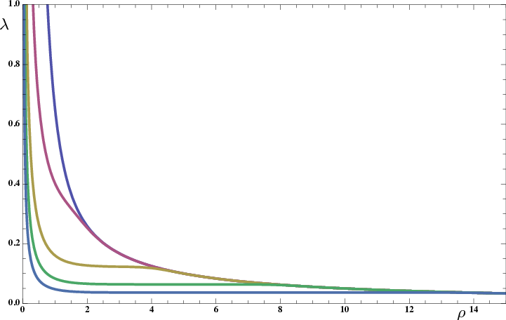
We plot in Fig. 2 the results obtained for the solution and the same sample of solutions as in Fig. 1. Notice the three distinct behaviors. Near the IR (), the running leads to a divergence. Near the UV (), the coupling is vanishing. In the intermediate region , where , the gauge coupling is effectively constant (walking).
III Five-dimensional supergravity formalism.
Following [7], we define new variables as
| (8) |
replace in the background equations from Eq. (1) and change the radial coordinate according to . The resulting system admits a consistent truncation to an effective 5-dimensional non-linear sigma model with fields coupled to gravity:
| (9) |
in a space-time of the form
| (10) |
IV Fluctuations, boundary conditions and numerical study
From here on, we work in units where . Following [7], after changing coordinates , writing the fluctuations as , replacing by (=) and using the equations for the 5d gravity fluctuations, we obtain the system of linearized equations for the scalar perturbations [8]
| (13) |
It is only for particular values of that the coupled differential equations (13) allow for solutions with acceptable IR and UV behavior. These give us the glueball spectrum of the dual field theory. In order to find them, we employ a numerical method described in [7], that in effect evolves solutions from both the IR and the UV, and then determines whether they match smoothly at a midpoint.
In the UV (for ), Eq. (13) can be diagonalized by a change to a basis in which the fluctuations behave as , where the exponents in general are non-integer, while
| (14) |
Notice that this behavior implies the presence of cuts in the two-point functions for and . We are interested here in the discrete spectrum, hence in the subleading behavior. We choose the minus signs in these expressions and use the result to set up the UV boundary conditions. Note that the consistent truncation used in [7], when studying the perturbations around , corresponds to keeping only the fluctuations that fall off as in the UV.
The following expansion of holds in the IR [6]:
| (15) |
where and are integration constants. Requiring that the background asymptotes to in the UV makes a function of (the analytical form of which is unknown).
We expand the fluctuations for as and plug them into the differential equation. The solutions are determined by the 12 integration constants , , , , , , , , , , , and , as
| (16) |
Regularity in the IR requires (taking (11) into account) and . We use Dirichlet boundary conditions for the first four fields.

The numerical results are plotted in Fig. 3. The spectrum for () consists of a series of poles approaching (in agreement with [7]). For large values of (equivalently, of ), all the masses in the series approach the branch points, so that the discrete spectrum effectively disappears into the continuum. With one notable exception: one of the states becomes lighter, and as is increased, its mass is pushed below both the continuum thresholds. For , this state becomes massless.
V Symmetry considerations
Expressing the five-dimensional background metric in terms of and yields
| (17) |
For , there exists a region where
| (18) | |||||
| (19) | |||||
| (20) |
and in this region the metric is approximated by
| (21) |
Defining the scaling transformation
| (22) | |||||
| (23) |
the metric is conformal to itself: .
This suggests that the light scalar might be a light dilaton, and hence its couplings should be dictated by this property. With present information, we are not able to reconstruct its composition in terms of the original degrees of freedom in the sigma-model. The metric is not asymptotically AdS in the UV, hence the rigorous procedure for holographic renormalization is not known, nor is it known how to characterize this state as normalizable or non-normalizable. A more detailed study of this and related points will be presented elsewhere [9].
VI Comments
This is not a walking technicolor theory, since it does not yield a mechanism for electro-weak symmetry breaking. However, the set of results collected here supports the idea that this system is a very interesting laboratory, in which walking can be studied systematically, and in which dynamical questions can be addressed in a calculable form, providing a guidance for model building.
The class of solutions we found yields the four-dimensional gauge coupling of a walking theory (the Lagrangian of which, for present purposes, we do not need to know), in the sense that there is an intermediate region where the gauge coupling is approximately constant. While the interpretation in terms of the dual field theory is at this point not well understood, the very fact that we observe a particle in the spectrum with a mass much lower than the dynamical scale of the theory (the main result of this paper) suggests that its existence is due to the spontaneous breaking of an approximate symmetry. If this symmetry is scale invariance, as suggested in the previous section, then the light scalar would be interpreted as the dilaton, the pseudo-Goldstone boson of dilatations. From the gravity point of view, it is clear that scale invariance is broken in the IR by the gaugino condensate, and in the UV at the scale set by .
Acknowledgements.
We thank A. Armoni, S. P. Kumar, and I. Papadimitriou for useful discussions. The work of MP is supported in part by WIMCS. The work of DE is supported in part by STFC Doctoral Training Grant ST/F00706X/1.References
- [1] B. Holdom, Phys. Lett. B 150, 301 (1985); K. Yamawaki et al. Phys. Rev. Lett. 56, 1335 (1986); T. W. Appelquist et al. Phys. Rev. Lett. 57, 957 (1986).
- [2] W. A. Bardeen et al. Phys. Rev. Lett. 56, 1230 (1986); M. Bando et al. Phys. Lett. B 178, 308 (1986); B. Holdom and J. Terning, Phys. Lett. B 187, 357 (1987); Phys. Lett. B 200, 338 (1988); W. D. Goldberger et al. Phys. Rev. Lett. 100, 111802 (2008).
- [3] J. M. Maldacena and C. Nunez, Phys. Rev. Lett. 86, 588 (2001).
- [4] C. Nunez et al. arXiv:0812.3655 [hep-th].
- [5] P. Di Vecchia et al. Nucl. Phys. B 646, 43 (2002); M. Bertolini and P. Merlatti, Phys. Lett. B 556, 80 (2003).
- [6] C. Hoyos-Badajoz et al. Phys. Rev. D 78, 086005 (2008). See also R. Casero et al. Phys. Rev. D 73, 086005 (2006); Phys. Rev. D 77, 046003 (2008).
- [7] M. Berg et al. Nucl. Phys. B 736, 82 (2006); Nucl. Phys. B 789, 1 (2008).
- [8] D. Elander, arXiv:0912.1600 [hep-th].
- [9] D. Elander et al., in preparation.