ANALYSIS AND COMPUTATION OF A DISCRETE KdV-BURGERS TYPE EQUATION WITH FAST DISPERSION AND SLOW DIFFUSION
Abstract.
The long time behavior of the dynamics of a fast-slow system of ordinary differential equations is examined. The system is derived from a spatial discretization of a Korteweg-de Vries-Burgers type equation, with fast dispersion and slow diffusion. The discretization is based on a model developed by Goodman and Lax, that is composed of a fast system drifted by a slow forcing term. A natural split to fast and slow state variables is, however, not available. Our approach views the limit behavior as an invariant measure of the fast motion drifted by the slow component, where the known constants of motion of the fast system are employed as slowly evolving observables; averaging equations for the latter lead to computation of characteristic features of the motion. Such computations are presented in the paper.
MSC Classification: 34E13, 34E15, 34C29, 35A35, 65L05, 65N22.
Keywords: singular perturbations, Young measures, multiscale computation, fast-slow systems.
1. Introduction
We consider the slow-fast system of ordinary differential equations
| (1.1) |
, with periodic boundary conditions , and where and are small parameters, such that in a sense that will be specified later. It is an elementary observation that (1.1) is a spatial discrete analogue of the classical Burgers’ equation
| (1.2) |
subject to periodic boundary conditions, with a basic domain , and is the size of the uniform mesh with points. But a more careful analysis (see, for example, Goodman and Lax [11]) shows that a higher order approximation of (1.1) is provided by the Korteweg-de Vries-Burgers’ type equation
| (1.3) |
with periodic boundary conditions
| (1.4) |
In section 2 we establish a formal derivation of (1.1) from (1.3), following Goodman and Lax [11]. This relation of (1.1) to (1.3), under the assumption that , reflects a competition between fast dispersion and slow diffusion mechanisms. Our goal in this paper is to find an effective equation governing the long time behavior of the “slow” diffusion, obtained via an “averaging” of the “slow” right hand side of (1.1) against the fast oscillations originating from the left hand side of (1.1). Intuition suggests that averaging will be relevant; however, implementing classical averaging results is not possible; we elaborate on this in the body of the paper, but note here that the source of the difficulty is to establish the existence and the identity of the “angle variables” in, say, a Hamiltonian representation, with respect to which averaging should be carried out. Solutions of (1.1) can be presented as images of solutions of a Hamiltonian system, but the latter are not bounded, so do not induce relevant information (this issue is discussed in section 3). Our approach relies on an alternative new theory of computing slow observables for singularly perturbed differential equations [3]. This theory has the distinct advantage of not requiring an explicit knowledge of the “angle variables” and for this problem will produce a system of equations for the slow observables of our approximate system of ordinary differential equations. The Lax invariants, which are traces of powers of a matrix component in a Lax pair, as developed systematically in Goodman and Lax [11] and the related work of Kac and van Moerbeke [13], are slow observables. We employ these and other invariants of the fast flow in the computations of the solutions of the discrete approximation.
The implementation of averaging techniques for systems of equations which are separated into fast and slow components is well known. These techniques in addition to component splitting often require explicit information on the fast dynamics, e.g. time periodicity, existence of limit cycles, or known stochastic behavior (see for example the survey of Givon, Kupferman, and Stuart [10], see also E et al. [8] and Kevrekidis et al. [14]). The issue of averaging in the absence of explicit knowledge of the fast dynamics was first considered by Artstein and Vigodner [7] in 1996 and continued in Artstein [1], [2], Artstein and Slemrod [5], [6]. A rigorous theory of averaging in the absence of both a component split and explicit limit characteristics of the fast dynamics was first given in [3]. The possible application of theory of [3] to a system with fast dispersion and slow diffusion was alluded to in [3] and this paper completes part of that program. In fact when the theory is coupled with techniques such as projective integration it provides, as we demonstrate in section 6, a fast and accurate method for computation of fast dispersion systems undergoing a slow perturbation. Of course our method does require some special features of the fast system, i.e. a rich family of first integrals of motion (invariants) of the type usually associated with, but not limited to, for instance, completely integrable Hamiltonian systems. System (1.1) is particularly interesting in that as far as available in the relevant literature, e.g. Moser and Zehnder [17], there is no known one-to-one correspondence between its fast part (when ) and a Hamiltonian system, nor do we know whether solutions of this fast system can be presented as the image of solutions of a Hamiltonian system with bounded dynamics. This fact renders the splitting into fast and slow components difficult at best and perhaps impossible.
The paper has five sections after this Introduction. Section 2 derives the semi-discrete approximation to the system in a manner suggested in the paper of Goodman and Lax [11]. It allows us to represent, in Section 3, the fast part of the system in terms of a Lax pair of matrices, thus producing a set of invariants of the fast dynamics. We also comment there on the Hamiltonian-type structure of the system. In section 4 we show that the positive orthant is invariant under the dynamics of the full system (1.1). Moreover, we use this fact to show the global existence of solutions to (1.1) with initial data in the positive orthant. In Section 5 we apply the theory of [3], displaying Young measure solutions to the limit problem, and the resulting evolution equations for the slow observables of our equation. Finally, in Section 6, we present numerical results for the relevant “effective slow” dynamics obtained in the limit as the parameter .
2. Derivation of the semi-discrete system
In this section we establish a formal derivation of (1.1) from (1.3) using the dispersive approximation scheme of Goodman and Lax [11] suitably modified for our viscous problem; for convenience of comparison we use the notation in [11].
For integers set . Hence periodicity of in implies is periodic in with period where . Assume is chosen so that is an even integer. Taylor’s theorem yields
| (2.1) |
and
| (2.2) |
Addition of (2.1) and (2.2) yields
| (2.3) |
while subtraction of (2.2) from (2.3) gives
| (2.4) |
Notice that the right hand sides of the latter two equations correspond to the expressions which constitute the continuous equation (2.1). Thus the continuous system (1.3) is formally equivalent to the semi-discrete, i.e., continuous in time only, discrete and -periodic in , system
| (2.5) |
with initial condition
| (2.6) |
(which is our original system (1.1)). The -periodicity means that in (2.5), and in equations later on, we use and . It is important to notice, though, that here the step size of the approximation and the dispersion coefficient are changed in a correlated way through the equality ; thus, a finer grid, namely, a larger but fixed , corresponds to a smaller dispersive coefficient; yet we always take
Goodman and Lax [11] examined the limit as of the non-viscous version of (1.3) via the analogous semi-discrete approximation. They proved, in particular, that during the time period prior to the formation of a shock in the KdV type equation, the solutions of the discrete approximation converge uniformly to the solution of the continuous one; but after the time instant when a shock forms in the Burgers equation, the discrete approximation generates oscillations. We consider equations (2.5)-(2.6) as the semi-discrete approximation of the KdV-Burgers equation (1.3); we wish to study the latter for fixed and as , namely, on long time intervals. To this end we rewrite (2.6) in the time scale , yielding
| (2.7) |
Denote by the vector ; system (2.7) can be rewritten as:
| (2.8) |
where
Now, in (2.8) (equivalently in (2.7)) we identify two contributions: The “fast part”, namely the vector field (for fixed), and the slow part, namely, , which corresponds to the diffusion.
3. Analysis of the fast equation
In this section we examine the “fast part” of the vector field determined by (2.7), i.e. we consider (2.7) after replacing its right hand side by zero. We seek to find invariants of the motion. These are not affected when multiplying the equation by a constant. Hence we write now the fast part of equation (2.7) suppressing the coefficient ; this amounts to a change of time scale, , without affecting other features of the dynamics; namely, we examine the equation
| (3.1) |
where and with even and with periodic boundary conditions (in particular, in (3.1) we interpret and ).
Observation 3.1.The product is an invariant of equation (3.1); also the product of the even coordinates and the product of the odd coordinates of the state, are invariants of equation (3.1). (We, actually, arrived at the above quantities guided by numerical simulations).
Proof. Straightforward, by showing that the time derivative of each of the terms is equal to zero (in fact, establishing invariance for two of the quantities implies that the third is also invariant).
Corollary 3.2. The positive orthant, determined by the condition for all , is invariant under the dynamics of (3.1) (later in the section we establish a stronger property).
In the closing paragraph of this section we identify Hamiltonian-type properties of the fast system (3.1). Now we identify first integrals of the fast dynamics, namely, constants of motion. To this end we review the results of Goodman and Lax [11] for the fast system, equation (3.1), and also borrow extensively from the presentation of Kac and van Moerbeke [13] and Moser [15], [16]; as far as the authors can tell the first representation of (3.1) in terms of Lax pairs was given by Moser [15], but, as was noted by Moser himself, it was analogous to that of Flaschka [9]. Moser, however, imposes Dirichlet boundary conditions while here we are interested in periodic boundary conditions; this case was also discussed in Moser and Zehnder [17].
We make a change of variables
| (3.2) |
With the additional change of time scale , the system (3.1) is transformed into
| (3.3) |
with periodic boundary conditions, hence in (3.3) and . We note that any positive solution of the system (3.1) can be rewritten as a solution of (3.3); by Corollary 3.2 the product is also an invariant of the equation. Hence the positive orthant in is invariant with respect to (3.3), and equations (3.1) and (3.3) are equivalent for solutions with positive initial data.
Now set , an -dimensional vector of real numbers, and extend periodically by .
Define the operation on elements as the translation and use the abbreviation ; likewise, is the translation in the opposite direction and .
Following Goodman and Lax [11], Kac and van Moerbeke [13] and Moser [15], [16], we associate with each vector the operators
| (3.4) |
where acts as a multiplication operator, i.e., when is written in its matrix representation then means that the -th row of is multiplied by the corresponding element, namely , of . The matrix is symmetric with diagonal elements equal to . For the convenience of the reader and further reference we give below the explicit terms when ; it should make the general case transparent.
| (3.5) |
With the aid of we now find conserved quantities for the equation (3.1). To this end define
| (3.6) |
which is anti-symmetric. Here . Furthermore, the commutator is given by
| (3.7) |
Note that (3.3) is equivalent to
| (3.8) |
Then, of course,
| (3.9) |
and more generally,
| (3.10) |
for any natural number . Since the right hand side of (3.10) is a commutator its trace is equal to zero. Therefore, for each we have
| (3.11) |
where signifies the trace. For odd the trace of is zero, so it does not reveal any information concerning equation (3.3). But for even, , the term is a nontrivial polynomial of degree . Thus, we have arrived at non-trivial conserved quantities, namely, first integrals, of equation (3.3). For example, the first two non-trivial traces for are
| (3.12) |
and
| (3.13) |
The last trace for the case is
| (3.14) |
Remark 3.3. As stated in Observation 3.1 the product of the is conserved by the equation (3.1); by (3.13) each of the stays uniformly bounded. Hence, for an initial condition with positive coordinates, the quantities along a trajectory are bounded and bounded away from zero; in particular, the solution exists for all time.
Remark 3.4. Invoking the relation (3.2), the invariants for (3.3) give invariants for (3.1). It is not easy to verify analytically that the invariants are functionally independent, namely, that they identify distinct dynamics; numerical simulations show, indeed, that their gradients are linearly independent, indicating their functional independence. In addition, and as noted in Observation 3.1, the following quantity is also an invariant of (3.1),
| (3.15) |
It has been shown by simple algebra for that the other invariants mentioned in Observation 3.1, namely
| (3.16) |
are not independent of the noted above and that this is hypothesized to be true for all even . Altogether we get functionally independent invariants. We do not know whether there are any independent global (i.e. not restricted to a specific lower dimensional manifold) first integrals in addition to the that we have identified; as we explain later on, the numerics indicates that the list is exhausted.
Considerations of the number of invariants may be significant as, under an appropriate transformation, solutions of (3.1) are differences of solutions of a completely integrable Hamiltonian system. This was noted in Goodman and Lax [11], referencing the work of Kac and van Moerbeke [13], Flaschka [9] and Moser [15], [16], see also Moser and Zehnder [17]. The technique follows a change of variables
| (3.17) |
under which the differential equation (3.1) takes the form
| (3.18) |
which we relate to the equation
| (3.19) |
via the relation
| (3.20) |
Observe that due to the periodicity of the ’s the sum of the ’s is zero, which might be a source for an extra invariant. Equation (3.19) is the well studied Toda lattice that forms a completely integrable Hamiltonian system. It is clear, however, from (3.19), that the solutions we are interested in, namely, solutions of (3.18), are differences of unbounded monotone increasing solutions (Moser [16] computes the asymptotics of these solutions). Due to the unboundedness, this Hamiltonian structure is not of much help in the computations of solutions of (3.1). We do not know if, possibly, another change of variables will induce a Hamiltonian structure on (3.1) or will make solutions of (3.1) images of bounded solutions of a Hamiltonian system.
4. A comment on the fast-slow system
In this section we show that the positive orthant is invariant with respect to the full fast-slow system (1.1). Moreover, we show that every such solution converges to a constant state .
Proposition 4.1. System (1.1) with for all , possesses a unique positive solution , for all . Moreover,
| (4.1) |
and converges to a constant, independent of , for all , as goes to infinity.
Proof. Since , for all , then for a short time we conclude from (1.1) that
| (4.2) | |||||
The last inequality is true since the function is monotone decreasing. Hence,
| (4.3) |
and
| (4.4) |
Consequently, for all , and for all .
Since in addition
| (4.5) |
we have uniformly bounded and hence we have global unique solutions. Finally, the expression is a Lyapunov function and via the well known LaSalle Invariance Principle (see, for example, [12], Chapter 10, Theorem 1.3, page 316) all solutions converge to the largest invariant set contained in the set defined by the solution of the algebraic equation
| (4.6) |
Since the only possible solutions to the above equality are , the proposition is proven.
5. Young measures solutions and observables of the fast-slow problem
In this section we address the full system (2.7). Let be arbitrary, but fixed. Based on the theory developed in [3] we represent limits, as , of solutions as Young measures over the interval ; then examine how slow observables of the system evolve over this arbitrary, but fixed, interval of time. The analysis is the basis for the computational developments in the closing section, section 6.
In the discussion that follows is fixed, hence is fixed. We will write for the vector in . We are interested then in limits of solutions of (2.7), as , over the interval .
The Young measures we use are defined on a time interval , with values being probability measures on , namely, on the state space of solutions of (2.7). For the relevant theory of Young measures see, e.g., [3] and references therein. A solution of (2.7), say , can be viewed as a Young measure when for each the vector is interpreted as a Dirac measure supported on . A Young measure can be viewed also as a measure on . Convergence of Young measures of the full fast-slow system (2.7), as , is interpreted as the weak convergence of the associated measures on ; the notion includes the case where a sequence of point-maps into , interpreted as Young measures, converge to a Young measure. Convergence of solutions of (2.7) in the sense of Young measures reflects that the distribution of the location of the solutions converge. In particular, the convergence in the sense of Young measures gives a more complete description of the limit behavior of the full system than the standard averaging method. This is because the Young measures approach provides a mathematical framework, i.e. in the sense of measures, for investigating and describing the limit behavior of both the slow as well as fast dynamics, while the averaging method restricts itself to the slow part of the dynamics.
The following result addresses the convergence of solutions in the sense of Young measures; its proof is based on the developments in previous sections and on [3], Theorem 4.4.
Theorem 5.1. Let the initial condition for (2.7) be given (alternatively, let be in a compact set in the positive orthant of ). Let be given, and fixed. Denote by the solution of (2.7), for a given , over the interval . Then a subsequence exists such that converge as , in the sense of Young measures on , to a Young measure, say , . Moreover, for almost every the measure is an invariant measure of the fast equation (3.1).
Proof. A straightforward computation shows that the quantity is not only an invariant of the fast flow (3.1), see (3.12), but also of the full equation (2.7) (indeed, it represents the total mass of the system, which, under periodic boundary conditions, is preserved under viscosity). Hence the family of functions, which is from into the positive orthant of , is bounded in . In particular, each solution in the sequence can be extended to the entire interval . Now the theorem follows from [3], Theorem 4.4.
The next result addresses the evolution of observables of the system. A measurement, or observable, is simply a function of . The notion of an orthogonal slow observable was defined in [3]; in our system it amounts to a measurement which is a first integral, namely, an invariant, of the fast equation (3.1). In Section 3 we identified such invariants. Denote by the invariants which are the traces of (see Section 3, but note that in that section the traces are expressed in terms of ); denote by the invariant given in (3.15). The invariance of each of the implies that whenever is an invariant measure of (3.1), the observed value is constant on the support of . We denote this value by .
Theorem 5.2. Let be as in the statement of Theorem 5.1 which converge, as , in the Young measures sense, to the Young measure , for . Denote = , namely, the measurement on the limit invariant measures. Then for each , the function satisfies the differential equation
| (5.1) |
where is the vector field given in (2.8), and the operator is with respect to the vector . Furthermore, the sequence of measurements converge weakly to , as , for .
Proof. The claims form a particular case of Theorem 6.5 in [3].
Under stronger conditions on continuity properties of the limit measure , the weak convergence in the previous result becomes a strong convergence; we do not pursue this here since in our system it is not easy to establish such continuity.
The differential equation (5.1) is not an autonomous ordinary differential equation since the limit measure is not determined by the observation . In some cases a set of observables determines the invariant measure; then, under continuity assumptions one can write an ordinary differential equation for this set of observables; without continuity a differential inclusion would determine the limit evolution of the observables. See Theorem 6.9 and Remark 6.11 in [3]. These results can be stated in our case employing the terms in (5.1), (2.8); we do not follow this direction since we do not know to what extent the observables we found form such a determining vector of observables. At any rate, the structure described here allows one to make progress toward a computational method, as displayed in the next section.
6. Computational study
In section we present a computational study of the theoretical tools that were developed in [3] and which were presented in the previous sections for system (2.7) (or equivalently (2.8)), with small values of . Specifically, we introduce two efficient numerical schemes for computing the evolution of the slow observables of (2.7), for small values of . In particular, we implement these schemes for computing the evolution of the slow observables , , that are discussed in section 5. Moreover, we demonstrate the computational efficiency of these algorithms in comparison to direct numerical simulations of the full system (2.7) for small values of . Both schemes are based on numerical evaluation of the time derivatives of the slow observables. That is, they are based on evaluating the time derivatives of the invariants of the fast system (3.1), , , as they are drifted by the slow field in (2.8).
In addition to the evolution of the slow observables, the method can simulate the evolution of the invariant measures of (3.1) themselves, thus getting a picture of the entire rapidly oscillating trajectories of (2.7).
The first approach, the Young measures approach, is based on computing the right hand side of (5.1). To this end, one has to compute first the invariant measures (see Theorem 5.1 and Theorem 5.2) of the fast system (3.1) by, for example, integrating system (3.1) for an appropriate interval of time, and then to advance , , numerically, according to the numerical evaluation of the right hand side of (5.1).
The second approach, the equation-free approach of [14] (it is equation-free since it avoids the direct use of any analytic form for the equation of evolution of the slow observables ), is based on numerically evaluating the time derivative of , , from the detailed simulator of the solution of the full fast-slow system (2.7), for small values of . It is worth mentioning, however, that the success of this method relies on the a priori knowledge that , are slow observables of (2.7) and that at the limit, when , their evolution is governed by a deterministic equation; that may not be at hand. These facts were established in the previous sections.
The efficiency of both algorithms stems from the fact one can take relatively large time steps for advancing the slow observables, in the first approach, and , for small values of , in the second approach. We call this step in both algorithms the projective step.
It is worth mentioning the philosophical difference between the two approaches. The first approach, which is based on Theorem 5.1 and Theorem 5.2, takes advantage of the fact that the evolution of the slow observables , , along the solution of system (2.7), are approximated, for small values of , by their corresponding limits , , as . Therefore, the first approach focuses on computing the slow observables of the limit equation, as . This is because the slow observables will then be considered as the approximations to the corresponding “real” slow observables , for small values of . The second approach, which is based on [14], deals, on the other hand, directly with system (2.7) without resorting to the limit equation, equation (5.1), but it implicitly assumes the existence of a limit equation.
Recall that in section 3 we established that there are at least invariants of the fast system (3.1), therefore each trajectory is constrained to a manifold of dimension at most . This appears to be achieved for the case of as shown in Figure 1,

which illustrates the solution of (3.1) for one initial value plotted in the first three variables, and . The solution lies on the surface of a 2-torus in this 3D projection. The same observation holds for all 3D projections of this case except those projections into either of all the odd-numbered or all the even-numbered coordinates (where it necessarily lies on the surface of one sheet of a two sheeted hyperboloid; this is because of the invariants noted in Observation 3.1). The trajectory “orbits” around the “long” direction of the torus, precessing from orbit to orbit. We assume, however, that we can approximate it, and the relevant invariant Young measure, , by integrating over an appropriate finite interval of time. Indeed, we have found that integrating for a few “orbits” over the “long” direction of the torus can give an adequate approximation for our application.
For a typical solution of (3.1) was found to be approximately a combination of two periodic motions, the fastest corresponding to an orbit around the long direction of the torus and the slow one corresponding to the precession time around the short direction. See, for instance, the graph of the first component, , of the solution of system (3.1) shown in Figure 2.

Whereas the general theory, as described in section 3, shows that there is a set of at least invariants for all solutions of the -dimensional problem (3.1), some particular solutions may satisfy additional invariants which we might call local invariants. That there are initial conditions leading to local invariants is easy to see. For instance, the case has 2 invariants ( and ). The case , the solutions of (3.1) that have started with , , and , will continue to maintain those identities along the trajectory and will have the same solution as the problem with those starting conditions. Hence its solution will lie on a one-dimensional manifold. This is shown in Figure 3. (The invariants in this case are the 2 invariants, for the case, and the 3 equalities, .) The case , for example, that is known to have at least 7 invariants, will have certain initial conditions with 10 invariants (corresponding to 2 copies of the case) or 11 invariants (corresponding to 3 copies of the case, or 4 copies of the case).

6.1. Two approaches for computing slow observables
In this subsection we illustrate in more detail the two approaches for computing the behavior of the fast-slow system (2.7) which we rewrite in the form
| (6.1) |
where is very small.
We do this for the case , but the technique is not restricted to that case. Both approaches are based on evaluating the time derivatives of the slow observables, , , as we have discussed above.
In the first approach, which is based on the Young measures as described in section 5, we utilize the right hand side of equation (5.1) to evaluate the “slow” derivatives of the slow observables , . This can be done by integrating the fast system (3.1), namely, the case of equation (6.1), to approximate the invariant Young measure of (3.1); what we practically do to evaluate the right hand side of (5.1) is to integrate over equally spaced time steps and approximate the integral in the right hand side of (5.1) by an averaged Riemann sum based on those points.
In the second approach, the equation-free method [14], we integrate the actual full fast-slow system equation (6.1) with small value of , compute the slow observables , , along the trajectory , which are guaranteed to be slow by our theory, and evaluate their slow derivatives by numerical differencing.
In both approaches we use the time derivative evaluation of the slow observables , , in order to advance them in time. We call this very last step in our scheme the “projective level”. We observe that the gain in the speedup of both schemes is due to the use of relatively large time steps at the projective level of the schemes for advancing the slow obervables. In order to repeat the process we need to initialize the detailed simulator (i.e., find initial conditions, , for the variables in the original -dimensional space) consistent with the “projected” values of the slow observables. That is, from the computed values of the slow observables, say , , we need to find a corresponding state variable , for which , for all . This procedure is called “lifting” in the equation-free literature [14]. In general this will involve the solution of a set of nonlinear algebraic equations with unknowns (and this implies that features of the solution can, in principle, be selected (almost) arbitrarily; in our six-dimensional example this “arbitrary” selection was implemented by carrying the values of two of the entries of the sought vector over from the last simulation.) As mentioned above, we take the point as an initial value for the corresponding system, i.e., an initial value for system (3.1) to compute the corresponding Young measure in the first approach, or an initial value for (6.1) to compute the corresponding solution in the second approach, and we repeat the above described process. Note that if is another point that has the same projected values of the slow observables as those of , i.e. , for all , then we are not guaranteed that the dynamics of the fast system (3.1) starting from will lead to the same invariant Young measure, , which is corresponding the trajectory starting from (see the relevant discussion regarding this matter in the closing paragraph of section 5). This is unless the invariant Young measure of (3.1) is unique, which is the case if the trajectory corresponding to the solution of fast dynamics (3.1) “fills” the manifold defined by the invariants of (3.1). As noted earlier, this manifold can be up to dimensional, since it is a sub-manifold of the manifold defined by the intersection of the invariant manifolds , ; although in reality it might be of lower dimension because of the additional local invariants.
6.2. The first approach - using the invariant Young measures
The invariants , , of the fast system (3.1) were identified in section 3 to be slow observables of the full fast-slow system (2.7), or equivalently of (2.8). Since these quantities are constants of motion for the fast dynamics, the contribution of the fast vector field, in (2.8), to their evolution is zero. Consequently, we focus only on computing the evolution of these slow observables as they are drifted by the slow vector field in (2.8). At the limit case, as , the rate of change of these slow observables, , is given by the right hand side of (5.1), that is, by the average of , the directional derivative of along the vector field , with respect of the Young invariant measure of the fast dynamics (3.1). The need to average over the measure can be seen from the wild fluctuation in Figure 4 of , for the 3rd Lax invariant , along the trajectory of the fast dynamics (3.1) that is shown in Figure 1.

As we mentioned earlier in the introduction of section 6, a typical solution of the fast dynamics (3.1) was found to be approximately a combination of two periodic motions, one fast and the other slower. The average value of along the trajectory of the fast dynamics (3.1), from the time to the current time, is shown in Figure 5. Either the time over which the average is taken has to be chosen carefully with respect to the approximate period of , or the average must be taken over a long time. In Figure 5 the circles indicate the averages at “periodic” points (the approximate fast period was estimated as 2.4868). Those dots indicate that we can get a reasonable approximation for the Young measure using a small number of approximate orbits.

We use this method of derivative evaluation of the slow observables, by virtue of the average over the Young’s measure in the right hand side of (5.1), in order to integrate them forward in time by simple forward Euler integration scheme with relatively large time steps. Then we compare the performance, i.e. speedup and efficiency, of this method to computing the slow observables through direct numerical simulation of the full fast-slow system (6.1) with , where the latter will be considered as a “true” solution. Computing the slow observables via the Young’s measure approach was done separately by first evaluating the time derivatives of the slow observables, as it was described above, over a fixed number of “fast periods”, and then advancing the slow observables by taking an integration step in a forward Euler scheme of either 3, 6, or 12 period length. We emphasize that the gain in the efficiency of this method lies in the last step, i.e. in the use of these relatively large time steps in advancing the slow observables forward in time. The solutions for the second through fourth slow observables, , over 3,000 “fast periods” (a time interval of 7,460.4) are shown in Figure 6. The slow observables of the “true” solution (found by integrating the full fast-slow system (6.1), with , and then computing the slow observables directly from it) are plotted as solid lines, while the integration of the slow observables via the Young’s measure method, as described above, are plotted as dotted lines; but the difference (to plot accuracy) is not visible.

We ran separate integrations over either 1, 2, 3, or 4 fast periods, in order to approximate the average in the right hand side of equation (5.1) with respect to the corresponding approximate invariant Young measures of the fast system (3.1). These separate integrations, or approximations of the Young measures, had less than a 10% effect on the solution errors. The dominant errors were due to the Euler integration. The errors in the slow observables after 600 fast periods are shown in Table 1.
| Euler step (periods) | |||
|---|---|---|---|
| 3 | 0.45 | 0.47 | 0.68 |
| 6 | 1.3 | 2.1 | 1.8 |
| 12 | 3.9 | 10.8 | 4.1 |
The speedup and efficiency of the Young measure integration scheme, in comparison to direct numerical simulation of the full fast-slow system (6.1), depends on the value of . The cost of evaluating the time derivative of the slow observables via the Young measure averaging in the right hand side of (5.1) is determined solely by the accuracy needed. Moreover, the number of integration steps needed for advancing the slow observables forward in time is also determined solely by the accuracy needed. However, if we were to integrate equation (6.1) directly, the number of time steps needed would be proportional to the integration interval which is proportional to . If, for example, we needed 50 integration steps for one approximate period, , and we wanted to track the dissipative (diffusion) terms until they had reduced by a factor of we would need to integrate from to (approximately). Since each approximate period is 2.4868 we would need about 4,600 periods, or 23,000 integration steps for a direct numerical integration of (6.1). If we used a higher-order integration method (rather than the first order Euler method used in this illustration) at the projective level, namely for advancing the slow observables in time after evaluating their time derivatives, we could probably integrate the decaying slow observables with much less than 100 projective steps - each of which requires one integration around of the fast system using 50 steps, for a total of 5,000 steps, or a speedup of better than 4 to 1. If were reduced by one tenth, the speedup would increase to better than 40 to one.
As mentioned, while computing the invariant measures of the fast system (3.1) (or equivalently of (6.1) with ) we actually simulate the entire evolution of the limit system of (6.1), as , via the supports of these measures - tori in our example. The decay of the tori of the full fast-slow system (6.1), with , can be seen in Figure 7 which shows the trajectories after 600, 1200, 1800, 2,400, and 3,000 fast periods of integration.


6.3. The second approach - the Equation-Free method
The equation-free method [14] utilizes the explicit knowledge of the numerical solution of (6.1), and consequently of the observables , , for short interval of time in order to approximate, here by numerical differencing, the time derivative of in order to project forward their values. The method is called equation-free since it does not use explicitly any equation of motion for the slow observables. However, it assumes that the evolution of is slow, and that there is an underlying process, or equation, that governs their evolution, which we do not use explicitly. (A valuable research direction would be to develop a method that identifies, possibly numerically, the slow observables in case they are not prescribed.)
For small values of the evolution of some of the slow observables, , , along solutions of (6.1) can exhibit a slight oscillatory behavior. For example, Figure 8 shows the early behavior of along the solution of equation (6.1) for the initial condition [1 1 1 1 4 1]. It exhibits a fine-scale oscillation. However, the values at the “periodic” points are reasonably smooth so we can use those points in order to evaluate the time derivative of the slow observables, , by numerical differencing. Then we use the numerical time derivatives of to project them forward in time. The results are illustrated in Figure 9. We show the results of projective integration of the slow observables (dotted lines) versus the evolution of the slow observables along a true solution of (6.1) (solid line) for the three slow observables and . Again, and as in the Young measure method, the results are indistinguishable to plot accuracy.
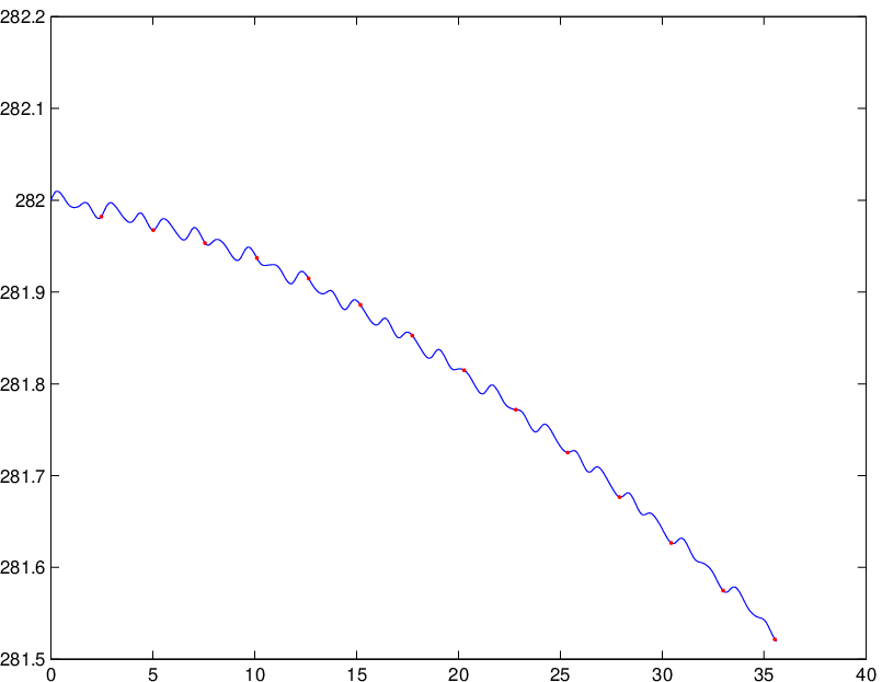

Table 2 shows the errors in the slow observables at using projective Euler integration by evaluating the time derivative from the slope of the chord over one period.
| Euler step (periods) | |||
|---|---|---|---|
| 3 | 0.8 | 3.6 | 0.5 |
| 6 | 1.9 | 5.9 | 1.8 |
| 12 | 4.2 | 14.2 | 3.9 |
Acknowledgements
The research of Z.A., I.G.K., M.S. and E.S.T. was supported by a grant from the United States - Israel Binational Science Foundation (BSF).
References
- [1] Z. Artstein, Singularly perturbed ordinary differential equations with nonautonomous fast dynamics, J. Dynamics and Differential Equations, 11 (1999), 297–318.
- [2] Z. Artstein, On singularly perturbed ordinary differential equations with measure-valued limits, Mathematica Bohemica, 127 (2002), 139–152.
- [3] Z. Artstein, I.G. Kevrekidis, M. Slemrod and E.S. Titi, it Slow observables of singularly perturbed differential equations, Nonlinearity, 20 (2007), 2463–2481.
- [4] Z. Artstein, J. Linshiz and E.S. Titi, Young measure approach to computing slowly advancing fast oscillations. Multiscale Modeling and Simulation 6 (2007), 1085–1097.
- [5] Z. Artstein and M. Slemrod, On singularly perturbed retarded functional differential equations, J. Differential Equations, 171 (2001), 88–109.
- [6] Z. Artstein and M. Slemrod, The singular perturbation limit of an elastic structure in a rapidly flowing nearly inviscid fluid, Quarterly of Applied Mathematics, 59 (2001), 543–555.
- [7] Z. Artstein and A. Vigodner, Singularly perturbed ordinary differential equations with dynamic limits, Proc. R. Soc. Edinb. A, 126 (1996), 541-69.
- [8] W. E, B. Engquist, X. Li, W. Ren and E. Vanden-Eijnden, Heterogeneous multiscale methods: A review, Comm. Comput. Phys., 2(3) (2007), 367–450.
- [9] H. Flaschka, The Toda lattice. II. Existence of integrals, Physical Review B, 9 (1974), 1924–1925.
- [10] D. Givon D, R. Kupferman and A. Stuart, Extracting macroscopic dynamics: model problems and algorithms Nonlinearity, 17 (2004), R55-R127.
- [11] J. Goodman and P. D. Lax, On dispersive difference schemes. I, Comm. Pure Appl. Math., 41 (1988), 591–613.
- [12] J. Hale, Ordinary Differential Equations, second edition, Krieger Publishing, Huntington, New York, 1980.
- [13] M. Kac and P. van Moerbeke, On an explicitly soluble system of nonlinear differential equations related to certain Toda lattices, Advances in Math., 16 (1975), 160–169.
- [14] I.G. Kevrekidis, C.W. Gear, J.M. Hyman, P.G. Kevrekidis, O. Runborg and K. Theodoropoulos, Equation-free coarse-grained multiscale computation: enabling microscopic simulators to perform system-level tasks, Comm. Math. Sciences, 1(4) (2003), 715–762.
- [15] J. Moser, Three integrable Hamiltonian systems connected with isospectral deformations, Advances in Math., 16 (1975), 197–220.
- [16] J. Moser, Finitely many mass points on the line under the influence of an exponential potential–an integrable system. In Dynamical Systems, Theory and Applications (Rencontres, BattelleRes. Inst., Seattle, Wash., 1974), pp. 467–497. Lecture Notes in Phys., Vol. 38, Springer, Berlin, 1975.
- [17] J. Moser and E.J. Zehnder, Notes on Dynamical Systems. Courant Lecture Notes in Mathematics, 12. New York University, Courant Institute of Mathematical Sciences, New York; American Mathematical Society, Providence, RI, 2005.