Generalized harmonic formulation in spherical symmetry

Preprint: AEI-2009-077

Matthew W. Choptuik Affiliation: Department of Physics and Astronomy, University of British Columbia Affiliation: 6224 Agricultural Road, Vancouver BC, Canada, V6T 1Z1 Affiliation: CIFAR Cosmology and Gravity Program Email: choptuik@physics.ubc.ca Affiliation: E-mail:

Abstract:

In this pedagogically structured article, we describe a generalized harmonic formulation of the Einstein equations in spherical symmetry which is regular at the origin. The generalized harmonic approach has attracted significant attention in numerical relativity over the past few years, especially as applied to the problem of binary inspiral and merger. A key issue when using the technique is the choice of the gauge source functions, and recent work has provided several prescriptions for gauge drivers designed to evolve these functions in a controlled way. We numerically investigate the parameter spaces of some of these drivers in the context of fully non-linear collapse of a real, massless scalar field, and determine nearly optimal parameter settings for specific situations. Surprisingly, we find that many of the drivers that perform well in 3+1 calculations that use Cartesian coordinates, are considerably less effective in spherical symmetry, where some of them are, in fact, unstable.

1 Introduction

Solving Einstein equations numerically is a notoriously difficult task. After many years of research, several well-posed formulations of the Einstein equations have been proposed and tested. These include constrained Arnowitt-Deser-Misner (ADM) [1, 2], hyperbolic Baumgarte-Shapiro-Shibata-Nakamura (BSSN) [3] and characteristic evolution [4], just to name a few: we refer the reader to [5, 6, 7] for reviews of these and other approaches. Among the ingredients that are key to the success of any particular formulation are 1) an appropriate choice of dynamic variables that results in a well-posed system, and 2) a choice of coordinates that remain regular during the course of the evolution. In this paper we focus on a specific well-posed approach known as the generalized harmonic (GH) formulation. This form of the Einstein equations has recently attracted significant attention in the numerical relativity community, in large part because of its use in obtaining the first long-term evolution of binary black-hole inspiral and merger [8, 9, 10].

In essence, the GH approach is a way to write the field equations such that the resulting system is manifestly hyperbolic, taking the form of a set of quasi-linear wave equations for the metric components. The basic idea underlying the strategy has a long and distinguished history: specifically, the use of harmonic coordinates has been instrumental in establishing many fundamental results in General Relativity (GR) including the characteristic structure of the theory [11], and the well-posedeness of the Cauchy problem for Einstein’s equations [12, 13]. However, from the computational point of view, harmonic gauge¹¹ 1 In this paper “gauge” means “coordinate choice”, and we use both expressions interchangeably. can be too restrictive, and numerical implementations using it may develop coordinate pathologies, as described, for instance, in [14] and [15]. More recently, it was realized by Friedrich [16], and independently by Garfinkle [17], that much of the coordinate freedom apparently lost by the specific choice of harmonic gauge could be regained through the introduction of certain gauge source functions, while at the same time maintaining the desirable property of strong hyperbolicity of the field equations. In fact, the source functions can be thought of as representing the coordinate freedom of the Einstein equations, and when constructing solutions of the equations, via an initial value approach, for example, they must be completely specified in some fashion.

Following Garfinkle’s pioneering use of the generalized harmonic approach in his study of generic singularity formulation in cosmologies with scalar field matter [17], the technique was successfully employed by Pretorius [8, 9, 10], and subsequently by others [18, 19, 20], for simulations of binary black hole coalescence. However, the total number of physical scenarios studied so far using the GH approach is limited, and there is an argument to be made for a more systematic exploration of the method’s potential. This is especially the case given the relative lack of proven prescriptions for choosing the gauge functions appropriately in instances where the gravitational field is highly nonlinear and dynamic. Moreover, in order to expedite experimentation with the approach, we feel that it is useful to start with systems with a high degree of symmetry. Restriction to highly symmetric spacetimes reduces the effective spatial dimensionality of the partial differential equations that must be solved, yields algebraically simpler equations, and, overall, leads to enormous savings in the computational resources required to simulate a single spacetime. This in turn allows for much more detailed and thorough surveys of the multi-dimensional parameter spaces that typically arise from a given choice of gauge functions.

In this paper, then, we focus on the application of the generalized harmonic approach to the problem of gravitational collapse in spherically symmetric $D$ -dimensional spacetime. Even with the restriction to spherical symmetry, we find that the strong-field aspects of the collapse process present significant challenges regarding the choice of the gauge functions. Ironically, some of these challenges may in fact be related to the symmetry restriction itself. As usual, in situations where a black hole forms, care must be taken to avoid the central singularity. This can be done through the use of singularity-avoiding coordinates, by excising the singularity from the computational domain, or with a combination of both strategies. Within the context of the GH formulation any such strategy must also be preserve the strong hyperbolicity of the field equations.

Although we view our study of the GH approach for spherically symmetric collapse as interesting in its own right, a primary goal of this research is to prepare for an investigation of axially symmetric systems using an analogous formulation. We thus consider our spherically-symmetric set up as a valuable toy model for the phenomenologically richer axisymmetric situation. In both cases it is natural to use coordinates in which the symmetries of the spacetime are explicit. These coordinates, however, are formally singular: at the origin in spherical symmetry, and on the axis in axial symmetry. Thus, in both instances the field equations have to be regularized in numerical implementations, and one of the results of our work is a regularization procedure that is compatible with the GH approach. Moreover, we expect that the experience gained from our spherically symmetric calculations concerning how to choose gauge source functions will also prove useful for the more general case of axisymmetric computations.

In order to maximize the usefulness of this paper to other researchers interested in experimenting with the generalized harmonic approach, we have attempted to make the following presentation reasonably self-contained and pedagogical in nature. We thus begin in Sec. 2 with a brief presentation of the basic GH formulae in full generality, along with a discussion of the constraint equations. Although the constraints are consistently preserved by the GH evolution equations in the continuum limit, in numerical calculations at finite resolution, deviations from the constraints generically develop. In order to maintain stability these deviations must be damped and we describe a method that effectively achieves this damping. Sec. 3 is devoted to a detailed discussion of coordinate conditions. One key issue that we consider is the non-trivial problem of prescribing the GH source functions to mimic some of the more popular and successful coordinate conditions that have historically been used in numerical relativity calculations. Following recent proposals [9, 10, 18, 19] we describe the formulation of the gauge conditions as hyperbolic evolution equations: is this approach the gauge functions are evolved, or “driven”, to desired targets in a controlled way, rather than being fixed instantly.

In Sec. 4 we adapt the GH formulae to the case of asymptotically flat, spherically symmetric configurations in $D$ spacetime dimensions. We derive the field equations, cast them into a form suitable for numerical solution, discuss initial and boundary conditions, and regularize the singular origin by introducing a new variable. Since we use spherical coordinates adopted to the symmetry, the GH source functions appear to diverge at the origin as $1/r$ . Hence, we regularize these functions as well by subtracting off the singular contribution that appears in the flat spacetime limit. The operators that appear in the various gauge drivers then act on the regularized source functions.

In order to endow our model with non-trivial dynamics, we introduce a minimally coupled, real, massless scalar field. The initial distribution of the scalar matter is freely specified and our results are grouped according to the “strength” of the initial data. In each case we simulate the time evolution of a single Gaussian pulse of scalar field that is initially centered at the origin. The weak and the intermediate data correspond to the dispersion of relatively dilute pulses, while a typical strong data configuration collapses to form a black hole or nearly does so.

Mathematically, the task of treating the coupled Einstein-scalar system involves the solution of a set of several quasi-linear wave equations. (Here we note that some of the gauge drivers involve auxiliary variables that obey first-order-in-time differential equations.) Our numerical approach to solving this system using finite difference techniques is detailed in Sec. 5. We compactify the spatial (radial) dimension into a finite region and cover it by a discrete lattice. This allows us to include spatial infinity on the finite difference mesh, which has the advantage of enabling us to set exact boundary conditions corresponding to asymptotic flatness. Following [8, 9] we directly discretize the second-order-in time-wave-equations on the mesh, and use a point-wise Gauss-Seidel relaxation method to update the discrete unknowns at each time step. In order to damp high-frequency components of the numerical solution—which can generically lead to instabilities—we incorporate explicit dissipation of the Kreiss-Oliger type. [31] This dissipation is also essential for attenuating spurious reflections from the outer region of the compactified domain that would otherwise quickly contaminate the solution in the interior (i.e. near the origin).

For the case of black hole formation we have investigated both of the approaches mentioned above for avoiding the central physical singularity. On the one hand, we have implemented an excision technique, in which an excision surface is chosen so that all characteristics on it are pointing inwards, obviating the need for explicit boundary conditions for the evolution equations. On the other hand, we have also experimented with the use of singularity avoiding slicing conditions, that “freeze” the evolution in the strong curvature regions. However, we find that in our case the calculations using singularity-avoiding slicings tend not to run as long as those with excision and appear to crash prematurely due to numerical errors that build up in the strong curvature regions.

Sec. 6 is devoted to a discussion of our detailed investigation of the performance of several coordinate conditions as applied to calculations involving various strengths of initial data. As already mentioned, the parameter spaces associated with many of the gauge drivers that we consider here are multidimensional. Thus, even with the significant reduction in needed computational resources that the restriction to spherical symmetry provides, we have not found it feasible to identify optimal parameters in all cases. In some instances then, we simply report what appears to be typical behavior for a particular gauge, while still trying to explore the effects of the variation of key parameters on the quality of the solutions. Interestingly, we find that several of the gauge drivers that have been successfully used in the $3+1$ simulations of black hole collisions that use Cartesian coordinates [9, 10, 18, 19] are considerably less effective for our spherically symmetric calculations. In particular, it is not always possible to drive the lapse to a certain value as reported in [9, 10], nor is it always possible to enforce a desired gauge for a long time by using one of the drivers described in [18]. Overall, our calculations seem to be more sensitive to the specific choices of parameters for the drivers than the Cartesian computations, and this is an issue which warrants further investigation.

Nevertheless, our results indicate that with a certain amount of parameter tuning, several of the gauge conditions that we investigate facilitate the simulation of many interesting scenarios. We are thus encouraged by this particular application of the generalized harmonic approach, and our conclusions and discussion in Sec. 7 includes an outline of some future extensions of the work.

2 Generalized harmonic formulation

We consider the Einstein equations on a $D$ -dimensional spacetime and written in the form

R_{\mu\nu}=8\pi G_{N}\bar{T}_{\mu\nu}\equiv 8\pi G_{N}\left(T_{\mu\nu}-\frac{1}{D-2}g_{\mu\nu}T\right),

(1)

where $g_{\mu\nu}$ is the metric, $R_{\mu\nu}$ is the Ricci tensor, $T_{\mu\nu}$ is the energy-momentum tensor of the matter with trace $T$ , and $G_{N}$ is the $D$ -dimensional Newton constant. Hereafter, we adopt units for which $8\pi G_{N}=1$ .

The Ricci tensor that appears in the left-hand-side of (1) contains various second derivatives of the metric components $g_{\mu\nu}$ : these second derivatives collectively constitute the principal part of $R_{\mu\nu}$ , viewed as an operator on $g_{\mu\nu}$ . This principal part can be decomposed into a term $g^{\alpha\beta}{\partial}_{\alpha\beta}g_{\mu\nu}$ , plus mixed derivatives of the form $g^{\alpha\gamma}{\partial}_{\alpha\mu}g_{\gamma\nu}$ . Without the mixed derivatives, (1) would represent manifestly (and strongly) hyperbolic wave equations for the $g_{\mu\nu}$ [21]. Strong hyperbolicity is a highly desirable property since mathematical theorems then ensure (local) existence and uniqueness of solutions at the continuum level. This, in turn, means that it should be possible to construct stable (convergent) numerical discretizations of the field equations.

One can view the generalized harmonic (GH) formulation of general relativity as a particular method that eliminates the mixed second derivatives appearing in (1) [16, 17, 8, 10, 22]. As the name suggests, the technique generalizes the harmonic approach in which the spacetime coordinates, $x^{\mu}$ , satisfy the harmonic coordinate condition

\Box x^{\alpha}=0.

(2)

Here we have

\Box x^{\alpha}=\frac{1}{\sqrt{-g}}{\partial}_{\nu}\left(\sqrt{-g}g^{\alpha\nu}\right)=-\Gamma^{\alpha}\equiv-g^{\gamma\beta}\Gamma^{\alpha}_{\gamma\beta},

(3)

where $\Gamma^{\alpha}_{\gamma\beta}$ are the usual Christoffel symbols.

It was realized by Friedrich [16] and also by Garfinkle [17], that it is possible to eliminate the mixed derivatives in the principal part of the Einstein equations while largely recovering the coordinate freedom than is lost by choosing the harmonic gauge. Instead of (2), one requires that that the coordinates satisfy

\Box x^{\alpha}=H^{\alpha},

(4)

where $H_{\alpha}\equiv g_{\alpha\beta}H^{\beta}$ are arbitrary ‘‘gauge source functions’’ ²² 2 In a slight abuse of notation and terminology we will refer to both $H_{\alpha}$ and $H^{\alpha}$ as “the” gauge source functions. which are to be viewed as specified quantities. One then defines the GH constraint

C^{\alpha}\equiv H^{\alpha}-\Box x^{\alpha},

(5)

which clearly must vanish provided (3) holds, and then modifies the Einstein equations as follows:

R_{\mu\nu}-C_{(\mu;\nu)}=\bar{T}_{\mu\nu}.

(6)

This last equation can be written more explicitly as

-{1\over 2}g^{\alpha\beta}g_{\mu\nu,\alpha\beta}-{g^{\alpha\beta}}_{(,\mu}g_{\nu)\beta,\alpha}-H_{(\mu,\nu)}+H_{\beta}\Gamma^{\beta}_{\mu\nu}-\Gamma^{\alpha}_{\nu\beta}\Gamma^{\beta}_{\mu\alpha}=\bar{T}_{\mu\nu}.

(7)

Now, provided that the $H_{\alpha}$ are functions of the coordinates and the metric only, but not of the metric derivatives—namely $H_{\alpha}=H_{\alpha}(x,g)$ —the field equations (7) form a manifestly hyperbolic system. We reemphasize that the source functions $H_{\alpha}$ are arbitrary at this stage and that their specification is equivalent to choosing the coordinate system for the spacetime under consideration (“fixing the gauge”). Determining an effective prescription for the source functions is thus crucial for the efficacy of the GH approach, and several strategies for fixing the $H_{\alpha}$ are discussed in the next section.

Having prescribed the coordinates we integrate the equations forward in time. Consistency of the scheme requires that the GH constraint (5) be preserved in time. The contracted Binachi identities guarantee that this is indeed the case, since, using those identities, one can show [8, 22] that $C^{\alpha}$ itself satisfies a wave equation,

\Box C^{\alpha}+{R^{\alpha}}_{\nu}\,C^{\nu}=0.

(8)

Thus, assuming that the evolution is generated from an initial hypersurface on which $C^{\alpha}={\partial}_{t}C^{\alpha}=0$ , (8) guarantees that $C^{\alpha}=0$ for all future (or past) times.

Although the GH constraint is preserved at the continuum level, in numerical calculations, where equations are discretized on a mesh with some characteristic mesh scale, $h$ , the constraint cannot be expected to hold exactly. More troublingly, experience shows that numerical solutions of (7)—particularly in strong field cases, such as those involving black holes—can admit “constraint violating modes”, with the result that the desired continuum solution is not obtained in the limit $h\to 0$ . Fortunately, an effective way of preventing the development of such modes in numerical calculations exists: one adds terms to the field equations that are explicitly designed to damp constraint violations (see e.g. [23]). In our implementation we follow Pretorius [8, 10] by adding constraint damping terms in a fashion inspired by studies of the so-called $\gamma$ -systems [24, 25]. The modified equations take the form

	$\displaystyle-{1\over 2}g^{\alpha\beta}g_{\mu\nu,\alpha\beta}$	$\displaystyle-$	$\displaystyle{g^{\alpha\beta}}_{(,\mu}g_{\nu)\beta,\alpha}-H_{(\mu,\nu)}+H_{\beta}\Gamma^{\beta}_{\mu\nu}-\Gamma^{\alpha}_{\nu\beta}\Gamma^{\beta}_{\mu\alpha}-$		(9)
		$\displaystyle-$	$\displaystyle\kappa\left(n_{(\mu}{\cal C}_{\nu)}-{1\over 2}g_{\mu\nu}\,n^{\beta}\,{\cal C}_{\beta}\right)=\bar{T}_{\mu\nu}.$		(9)

Here, $n^{\alpha}$ is the future-directed, unit time-like vector normal to the $t={\rm const.}$ hypersurfaces, which can be written as

n_{\alpha}\equiv-\left(1/\sqrt{-g^{tt}}\right){\partial}_{\alpha}t,

(10)

and $\kappa$ is an adjustable parameter that controls the damping timescale. Specifically, as discussed in [25], small constraint perturbations about a fixed background decay exponentially with a characteristic timescale of order $\kappa$ . We note that the constraint damping term contains only first derivatives of the metric and hence does not affect the principal (hyperbolic) part of the equations.

3 Coordinate conditions

As we have already mentioned, fixing the coordinates in the GH approach amounts to specifying the source functions $H_{\alpha}$ . In this regard, it is instructive to examine the relationship between the $H_{\alpha}$ and the lapse function and shift vector that appear in the ADM, or space-plus-time, formulation of general relativity. We recall that in the ADM formalism the line element can be written as

ds^{2}=-\alpha^{2}dt^{2}+\gamma_{ij}\left(dx^{i}+\beta^{i}dt\right)\left(dx^{j}+\beta^{j}dt\right),

(11)

where $\alpha$ is the lapse function, $\beta^{i}$ is the shift vector, and $\gamma_{ij}$ is the spatial metric of the $t={\rm const.}$ hypersurfaces. Using this form of the spacetime metric in (4) yields

	$\displaystyle{\partial}_{t}\alpha-\beta^{k}{\partial}_{k}\alpha$	$\displaystyle=$	$\displaystyle-\alpha\left(H_{n}+\alpha K\right),$
	$\displaystyle{\partial}_{t}\beta^{i}-\beta^{k}{\partial}_{k}\beta^{i}$	$\displaystyle=$	$\displaystyle\alpha\gamma^{ij}\left[\alpha\left(H_{j}+{{}^{(D-1)}}\Gamma_{jkl}\gamma^{kl}\right)-{\partial}_{j}\alpha\right],$		(12)

where $H_{n}\equiv n^{\mu}H_{\mu}=(H_{t}-\beta^{i}H_{i})/\alpha$ is the normal component of the source function $H_{\mu}$ , $K$ is the trace of the extrinsic curvature tensor of the $t={\rm const.}$ slices, and the ${}^{(D-1)}\Gamma_{jkl}$ are Christoffel symbols associated with the spatial $\gamma_{ij}$ . Bearing in mind that the temporal component of the source function is thus determined by $H_{t}=\alpha\,H_{n}+\beta^{i}H_{i}$ , these last equations clearly exhibit the connection between the gauge source functions and the time evolution of the lapse and shift.

In his groundbreaking application of the GH approach [9, 10], Pretorius used insight derived from considering this relationship between the $H_{\alpha}$ and the ADM kinematic variables to devise a methodology that generates effective gauge source functions for the problem of binary black hole collisions. His strategy elevates the status of the $H_{\alpha}$ to independent dynamical variables that satisfy time-dependent partial differential equations. Crucially, the evolution equations for the $H_{\alpha}$ are designed so that the lapse and shift which (implicitly) result from the time development have certain desirable properties. For example, the equation for $H_{t}$ is tailored in an attempt to keep the value of the lapse function of order unity everywhere—including near the surfaces of the black holes—during the evolution.

One specific prescription for achieving this type of control evolves the gauge source functions according to

	$\displaystyle\Box H_{t}$	$\displaystyle=$	$\displaystyle-\xi_{1}\,\frac{\alpha-\alpha_{0}}{\alpha^{q}}+\xi_{2}\,H_{t,\mu}n^{\mu},$
	$\displaystyle H_{i}$	$\displaystyle=$	$\displaystyle 0,$		(13)

where $\Box$ is the covariant wave operator, and $\alpha_{0},\xi_{1},\xi_{2}$ and $q$ are adjustable constants³³ 3 Sometimes it is convenient to assume that $\xi_{1}$ and $\xi_{2}$ are given functions of space and time rather than mere constants. For example, one might require that the gauge driver is switched on gradually in time, or that it be active only in certain regions, e.g. in the vicinity of a black hole, and that its effect vanish asymptotically, so that pure harmonic coordinates are recovered at large distances. . Thus the temporal source function satisfies a wave equation similar to those that govern the metric components in the system (9). The first term on the right-hand-side of (13) is designed to “drive” $H_{t}$ to a value that results in a lapse that is approximately $\alpha_{0}$ . The second, “frictional” term tends to confine $H_{t}$ to this value. For the case of the spatial coordinates, Pretorius found that the simplest choice of spatially harmonic gauge— $H_{i}=0$ —was sufficient in simulations of binary black hole collisions. Importantly, the choice (13) ensures that the hyperbolicity of the combined evolution system is preserved. A slight generalization of this technique was considered in [19] where instead of using $H_{i}=0$ , the spatial components of the source functions are evolved according to

\Box H_{i}=-\xi_{3}\,\frac{\beta_{i}}{\alpha^{2}}+\xi_{2}\,H_{i,\mu}n^{\mu}

(14)

where $\xi_{3}$ is an additional parameter.

One possible problem with the specific driver approach outlined above is that the coordinates that result do not correspond to those produced by any of the more familiar coordinate conditions typically used in numerical relativity. Recently, Lindblom et al [18] proposed driver conditions that are crafted so that the source functions that result imply particular conditions on the corresponding lapse and shift. We now proceed to a review of this interesting and promising approach.

We begin by observing that many traditional coordinate conditions of numerical relativity can be written as $F_{\alpha}=F_{\alpha}(x,g,{\partial}g)$ where the $F_{\alpha}$ are to be viewed as “effective” gauge source functions which could be computed, for example, were the entire spacetime in hand. Within the GH approach, enforcing such a condition algebraically by simply setting $H_{\alpha}=F_{\alpha}$ will generally destroy the hyperbolicity of the system, since the $H_{(\mu;\nu)}$ terms in (7) will generically give rise to mixed second derivatives of the metric. Lindblom et al circumvent this difficulty by generalizing (13) to

{\cal O}H_{\alpha}=Q_{\alpha}(x,g,{\partial}g,H,{\partial}H),

(15)

where ${\cal O}$ is a second order hyperbolic operator and $Q_{\alpha}$ is chosen so that the source functions evolve towards the concrete $F_{\alpha}=F_{\alpha}(x,g,{\partial}g)$ that define the desired gauge. The combined system (9) and (15) will remain hyperbolic provided the $Q_{\alpha}$ depend on at most first derivatives of the fields. In analogy with (13) the authors of [18] choose

Q_{\alpha}=\mu_{1}^{2}\,\left(H_{\alpha}-F_{\alpha}\right)+2\mu_{2}\,{\partial}_{t}H_{\alpha}+\eta\,W_{\alpha},

(16)

where $\mu_{1},\mu_{2}$ and $\eta$ are adjustable parameters, and $W_{\alpha}$ is assumed to satisfy

{\partial}_{t}W_{\alpha}+\eta\,W_{\alpha}=\hat{{\cal O}}H_{\alpha},

(17)

where $\hat{{\cal O}}$ is the part of ${\cal O}$ that contains only spatial derivatives. When the spacetime is stationary, time-derivatives vanish and equations (15) and (16) then imply $H_{\alpha}=F_{\alpha}$ . Notice that without the introduction of the auxiliary fields, $W_{\alpha}$ , this property could not be attained for general, position dependent gauges [18].

In order to implement this method for a specific desired gauge choice one must first compute the corresponding target source functions, $F_{\alpha}$ . Here we focus on gauges of the schematic form $G_{\alpha}(x,g,{\partial}g)=0$ for which one can choose [18]

F_{\alpha}=-\Gamma_{\alpha}-q\,G_{\alpha},

(18)

where $q$ is a tunable parameter. In the GH formalism, $H_{\alpha}=-\Gamma_{\alpha}$ , and (18) then implies $H_{\alpha}-F_{\alpha}=q\,G_{\alpha}$ . This demonstrates that when the GH constraint is satisfied, $H_{\alpha}$ is driven to $F_{\alpha}$ if $G_{\alpha}$ is driven to zero. We next discuss several specific coordinate choices that are explored in this paper.

3.1 Slicing conditions

For the particular choices of the slicing conditions that we use in this paper, it is more convenient to calculate the normal component of the target source functions, $F_{n}\equiv n^{\mu}F_{\mu}=(F_{t}-\beta^{i}F_{i})/\alpha$ , than the temporal component, $F_{t}$ , itself (see (12)). Once this is done, then in conjunction with the shift conditions that fix $F_{i}$ , the temporal component can be easily computed via $F_{t}=\alpha F_{n}+\beta^{i}F_{i}$ .

•

Constant curvature slicing, $K=K_{0}$ . Here we assume that the trace, $K(g,{\partial}g)$ , of the extrinsic curvature of the spatial slices is constant. When $K_{0}=0$ , we have the famous maximal slicing condition [28] whose significant popularity in numerical calculations is due in large part to the strong singularity-avoiding property exhibited by the resulting constant-time surfaces (see Sec. 6). The constant curvature foliation can be written as $G_{n}=0$ , where

$G_{n}=K_{0}-K=K_{0}+\nabla^{\alpha}n_{\alpha}$ (19)
•

Bona-Masso slicing [30]. This condition can be written as

$G_{n}=({\partial}_{t}\alpha-\beta^{i}{\partial}_{i}\alpha)+\alpha^{2}f(\alpha)\left(K-K_{0}\right),$ (20)

where $f(\alpha)$ is an arbitrary function of the lapse.⁴⁴ 4 Sometimes the geometric derivative ${\partial}_{n}\alpha\equiv({\partial}_{t}\alpha-\beta^{i}{\partial}_{i}\alpha)/\alpha$ is replaced with the partial time derivative ${\partial}_{t}\alpha$ . The choice $f(\alpha)=2/\alpha$ corresponds to the popular $1+\log$ slicing.

In terms of implementing these slicing conditions, we note that (18) implies

F_{n}=-\alpha^{-1}\left(\Gamma_{t}-\beta^{i}\Gamma_{i}\right)-q_{n}\,G_{n},

(21)

where $q_{n}$ is a parameter, and that the kinematic quantities such as the lapse and shift which appear in various formulae above can always be written in terms of the fundamental dynamical variables of the scheme (i.e. the metric components and their first derivatives).

3.2 Shift conditions

An important class of shift conditions which is often used in numerical relativity employs versions of the so-called $\Gamma$ -driver [27]. In this approach, one first introduces the conformally rescaled spatial metric, $\tilde{\gamma}_{ij}=\gamma^{\sigma}\gamma_{ij}$ , with $\gamma\equiv\det\gamma_{ij}$ and $\sigma$ an arbitrary parameter, then computes the contracted Christoffel symbols,

^{(D-1)}\tilde{\Gamma}^{i}=^{(D-1)}\tilde{\Gamma}^{i}_{kj}\tilde{\gamma}^{kj}=-\gamma^{-\sigma}\left[\frac{1+\sigma\,(D-3)}{2}\gamma^{ij}{\partial}_{j}\log\gamma+\gamma^{i}_{j}{\partial}_{k}\gamma^{kj}\right],

(22)

and imposes certain conditions on their dynamics. The $\Gamma$ -driver strategy is related to the minimal distortion condition [28, 29] which is designed to minimize the time variation of $\tilde{\gamma}_{ij}$ (see e.g. [27]).

•

$\Gamma$ -freezing. Here one requires

${\partial}_{t}\,^{(D-1)}\tilde{\Gamma}^{i}=0,$ (23)

which implies that during the evolution ${}^{(D-1)}\tilde{\Gamma}^{i}$ is fixed, ${}^{(D-1)}\tilde{\Gamma}^{i}=^{(D-1)}\tilde{\Gamma}^{i}|_{t=0}$ . Following [18] we attempt to evolve to this choice by choosing

$G_{i}=\tilde{\gamma}_{ij}\left({}^{(D-1)}\tilde{\Gamma}^{j}(0)-^{(D-1)}\tilde{\Gamma}^{j}\right).$ (24)

•

$\Gamma$ -driver. Again following [18] we write the driver condition as

	$\displaystyle{\partial}_{t}\beta^{i}$	$\displaystyle=$	$\displaystyle\nu\left[{}^{(D-1)}\tilde{\Gamma}^{i}-\eta_{2}\,B^{i}\right],$		(25)
	$\displaystyle{\partial}_{t}B^{i}$	$\displaystyle+$	$\displaystyle\eta_{2}\,B^{i}=^{(D-1)}\tilde{\Gamma}^{i},$		(26)

where $\nu$ and $\eta$ are adjustable parameters. Then one can choose

G_{i}=\gamma_{ij}\left({\partial}_{t}\beta^{j}-\nu\,^{(D-1)}\tilde{\Gamma}^{j}+\nu\eta_{2}\,B^{j}\right),

(27)

The auxiliary variable $B^{i}$ is evolved using (26) and it is important to note that adding this equation to the scheme does not destroy the hyperbolicity of the combined evolution system [18].

We have also experimented with a geometric version of the driver where the partial time derivative ${\partial}_{t}$ in (26) is replaced with the covariant derivative $n^{\mu}\nabla_{\mu}\equiv({\partial}_{t}-\beta^{k}{\partial}_{k})/\alpha$ .

Implementation of the above shift conditions is effected by setting the corresponding spatial target source function defined by (18) according to

F_{i}=-\Gamma_{i}-q_{i}\,G_{i},

(28)

where $q_{i}$ is an adjustable parameter.

4 Spherically-symmetric reduction

Having described the basics of the GH formalism, we now specialize to spherically symmetric spacetimes. We consider a $D$ -dimensional spacetime with $SO(D-2)$ rotational symmetry, and write the $D$ -dimensional line element in the form

ds^{2}=g^{(D)}_{\mu\nu}dx^{\mu}dx^{\nu}=g^{(D)}_{ab}dx^{a}dx^{b}+e^{2\,\hat{S}}d\Omega_{n}^{2}.

(29)

Here $d\Omega_{n}^{2}$ is the metric on a unit n-sphere, $n\equiv D-2$ , $a,b=\{t,r\}$ , and the metric $g^{(D)}_{ab}$ and scalar $\hat{S}$ are functions of $t$ and the radial coordinate, $r$ , alone.

Although we will later specialize to the case of a real, massless scalar field, for generality we first adopt as a matter source minimally coupled complex scalar field, $\Phi$ , with a potential $V(|\Phi|)$ . The action that describes the system can be written as

S=\int\sqrt{-g^{(D)}}\left(R^{(D)}-{\partial}_{a}\Phi\,{\partial}^{a}\Phi^{*}-2\,V(|\Phi|)\right)dx^{D}.

(30)

By varying the action with respect to the fields one gets the Einstein equations (1) with the energy-momentum tensor $\bar{T}_{\mu\nu}={1\over 2}\left({\partial}_{\mu}\Phi\,{\partial}_{\mu}\Phi^{*}+{\partial}_{\mu}\Phi^{*}\,{\partial}_{\mu}\Phi\right)+2/(D-2)g_{\mu\nu}^{(D)}\,V$ , as well as the general relativistic Klein-Gordon equation for the scalar field. Specifically, the GH transformation of the Einstein equations as given by (6) reads

	$\displaystyle R^{(D)}_{ab}-C_{(a;b)}={1\over 2}\left({\partial}_{a}\Phi\,{\partial}_{b}\Phi^{}+{\partial}_{a}\Phi^{}\,{\partial}_{b}\Phi\right)+\frac{2}{D-2}g_{ab}^{(D)}\,V,$		(31)
	$\displaystyle R^{(D)}_{\theta_{i}\theta_{i}}-C_{(\theta_{i};\theta_{i})}=\frac{2}{D-2}g_{\theta_{i}\theta_{i}}^{(D)}\,V,$		(32)
	$\displaystyle\Box\Phi={\partial}V/{\partial}\Phi^{*},$		(33)

where $R^{(D)}_{\mu\nu}$ is the $D$ -dimensional Ricci tensor and $\theta_{i}$ are the angular coordinates. In spherical symmetry it suffices to use any specific angular component of the Ricci tensor, and for convenience we use $R^{(D)}_{\theta_{1}\theta_{1}}$ where $\theta_{1}$ is defined by $d\Omega_{n}^{2}=d\theta_{1}^{2}+\sin^{2}\theta_{1}d\Omega_{n-1}^{2}$ .

The form of the metric (29) is not yet optimal for use in numerical computations. In this paper we are mostly interested in asymptotically flat solutions and thus the following section describes a more natural ansatz for use in that instance.

4.1 Spatial asymptotics

In spherical coordinates, flat spacetime can be written as

ds^{2}=-dt^{2}+dr^{2}+r^{2}\,d\Omega_{n}^{2}.

(34)

It follows from (29) that asymptotically $g_{ab}\rightarrow\eta_{ab}$ , where $\eta_{ab}$ is a Minkowski metric, and $\hat{S}\rightarrow\log\,r$ , (i.e. $\hat{S}$ diverges at spatial infinity). Since this divergence complicates the numerical implementation of boundary conditions, we introduce a new function, $S$ , defined by $S=\hat{S}-\log\,r$ , which is regular everywhere. We then adopt the following, more regular form for the line element in the asymptotically flat case:

ds^{2}=g_{ab}dx^{a}dx^{b}+r^{2}\,e^{2\,S}d\Omega^{2}_{n}.

(35)

In spherical coordinates, the source function derived from (4) does not vanish even in flat spacetime where it becomes

H^{\rm Mink}_{\mu}=-\Gamma^{\rm Mink}_{\mu}=(0,n/r,(n-1)\,\cot\theta_{1},(n-2)\,\cot\theta_{2},\dots,\cot\theta_{n-1},0).

(36)

Since near the origin spacetime is locally flat, the radial component of the source function is generically singular at $r=0$ , diverging as $n/r$ . To regularize this radial component, we thus subtract the singular background contribution by transforming $H_{\alpha}\to H_{\alpha}+\delta^{r}_{\alpha}H_{r}^{\rm Mink}$ , and use the functions $H_{t}$ and $H_{r}$ defined by

H_{\alpha}=\left(H_{t}(t,r),H_{r}(t,r)+n/r,(n-1)\cot\theta_{1},(n-2)\,\cot\theta_{2},\dots,\cot\theta_{n-1},0\right).

(37)

in our formulae.

With the line-element (35) and the source functions (37), the asymptotic behavior of the fields is simply

g_{ab}\rightarrow\eta_{ab},~~~S\rightarrow 0,~~~\phi\rightarrow 0,~~~H_{t}\rightarrow 0,~~~H_{r}\rightarrow 0

(38)

In App. A we also analyze the asymptotically AdS spacetime, which is described in our model (30) for the case that the scalar field potential satisfies $V(0)\rightarrow\Lambda<0$ .

4.2 Center of symmetry, $r=0$

Invariance of the line element (35) under the reflection $r\rightarrow-r$ in spherical symmetry implies that $g_{tr}$ is an odd function of $r$ , while $g_{tt},g_{rr},S$ and $\Phi$ are even in $r$ . Additionally, the GH constraint (4) implies that the source functions $H_{r}$ , regularized via (37), and $H_{t}$ are odd and even in $r$ , respectively.

Moreover, the requirement that the surface area of an $n$ -sphere must vanish at the origin⁵⁵ 5 that is, that the radial and areal coordinates coincide at the origin, to avoid a conical singularity there. implies $g_{rr}(t,0)=e^{2\,S(t,0)}$ . We note that this is an extra condition on $S$ , which thus has to satisfy both this relation, as well as the constraint that it have vanishing radial derivative at $r=0$ —specifically that $g_{rr}-e^{2\,S}=O(r^{2})$ . Therefore, at $r=0$ we essentially have three conditions on the two fields $S$ and $g_{rr}$ . In the continuum, and given regular initial data, the evolution equations will preserve regularity: however, in a numerical code that solves the equations discretized on a lattice, this will be true only up to discretization errors. As a general rule-of-thumb, the number of boundary conditions should be equal to the number of evolved variables in order to avoid regularity problems and divergences of a numerical implementation.

An elegant way to deal with this regularity issue involves definition of a new variable, $\lambda$ : ⁶⁶ 6 We note that a similar variable was introduced in [26], also for the purpose of regularization.

\lambda\equiv\frac{g_{rr}-e^{2\,S}}{r}.

(39)

At the origin one then has $\lambda\sim O(r)$ . Therefore, after changing variables from $S$ to $\lambda$ by using $S=(1/2)\log(g_{rr}-r\,\lambda)$ in all equations, and imposing $\lambda(t,0)=0$ at the origin, one ends up with a system where there is no over-constraining due to the demand of regularity at $r=0$ . In addition, we note that at spatial infinity we have $\lambda=0$ , and that the hyperbolicity of the GH system is not affected by the change of variables.

However, as described in detail in Sec. 5.2, we were able to implement a more straightforward regularization method that maintains $S$ as a fundamental dynamical variable, and thus opted to use that approach in our current calculations.

4.3 The equations

With the metric ansatz (35) and the regularized source function (37), equations (31)–(33) become 5 equations for the 5 variables, $g_{tt},g_{tr},g_{rr},S$ and $\Phi$ , that schematically can be written as⁷⁷ 7 Using $\lambda$ instead of $S$ does not change this structure since the equation that governs $\lambda$ is a linear combination of the equations that govern $S$ and $g_{rr}$ .

	$\displaystyle-{1\over 2}g^{cd}g_{ab,cd}+\dots={1\over 2}\left({\partial}_{a}\Phi\,{\partial}_{b}\Phi^{}+{\partial}_{a}\Phi^{}\,{\partial}_{b}\Phi\right)+\frac{2}{D-2}g_{ab}V,$		(40)
	$\displaystyle g^{cd}S_{,cd}+\dots=-\frac{2}{D-2}\,V,$		(41)
	$\displaystyle g^{cd}\Phi_{,cd}+\dots={\partial}V/{\partial}\Phi^{*}.$		(42)

Here ellipses denote terms that may contain the metric and/or the source functions, as well as their first derivatives in various combinations (see App. B for the explicit set of equations in the four-dimensional case). These equations are to be evolved forward in time starting from the initial ( $t=0$ ) time slice, where values for the fields and their first time derivatives must be prescribed.

4.4 Coordinate choices

Here we adapt the prescriptions for choosing the gauge functions ( $H_{t}$ and $H_{r}$ ) that were described in Sec. 3, to the case of spherical symmetry. We again note that the radial source function is singular at the origin in spherical symmetry, and that we thus regularize it via (37). Since this regularization involves subtracting the flat-spacetime singular part from $H_{r}$ , any specific coordinate conditions discussed here are thus defined relative to spherical Minkowski spacetime.

For the case of the gauge condition (13) inspired by Pretorius’ original work, we have

	$\displaystyle\Box H_{t}$	$\displaystyle=$	$\displaystyle-\xi_{1}\,\frac{\alpha-\alpha_{0}}{\alpha^{q}}+\xi_{2}\,\left({\partial}_{t}H_{t}-\beta\,{\partial}_{r}H_{t}\right)/\alpha,$		(43)
	$\displaystyle H_{r}$	$\displaystyle=$	$\displaystyle 0.$

Similarly for the modification of the above proposed in [19], we have (using (14))

	$\displaystyle\Box H_{t}$	$\displaystyle=$	$\displaystyle-\xi_{1}\,\frac{\alpha-\alpha_{0}}{\alpha^{q}}+\xi_{2}\,\left({\partial}_{t}H_{t}-\beta\,{\partial}_{r}H_{t}\right)/\alpha,$		(44)
	$\displaystyle\Box H_{r}$	$\displaystyle=$	$\displaystyle-\xi_{3}\,\frac{\beta}{\alpha^{2}}+\xi_{2}\,\left({\partial}_{t}H_{r}-\beta\,{\partial}_{r}H_{r}\right)/\alpha.$

In the above equations $\Box$ is the regularized scalar wave operator in spherical symmetry, given by

\Box\,H_{\alpha}=g^{\mu\nu}{\partial}_{\mu}{\partial}_{\nu}H_{\alpha}-\left(\Gamma^{\nu}+g^{rr}\,\frac{n}{r}\delta^{\nu}_{r}\delta^{\alpha}_{r}\right){\partial}_{\nu}\,H_{\alpha}.

(45)

Turning now to the case of the gauge drivers introduced by Lindblom et al, we note that the operator in (37) is essentially the vector d’Alambertian⁸⁸ 8 $H_{a}$ does not transform as a vector under gauge transformations, so the equation should be understood as written in particular global coordinates [18]; in the current case, these are our spherical coordinates. [18]

{\cal O}\,H_{\alpha}=g^{\mu\nu}{\partial}_{\mu}{\partial}_{\nu}H_{\alpha}-\Gamma^{\nu}{\partial}_{\nu}H_{\alpha}-2\,g^{\mu\nu}\Gamma^{\beta}_{\nu\alpha}{\partial}_{\mu}H_{\beta}+\left(R_{\alpha}^{\beta}-{\partial}_{\alpha}\Gamma^{\beta}\right)\,H_{\beta}.

(46)

In order to avoid having second-derivatives of the metric, the Ricci tensor in the last term should be thought of as being determined by matter sources and replaced with $\bar{T}_{\alpha}^{\beta}$ , in accordance with the Einstein equations. In addition, using the GH constraint $H_{\alpha}=-\Gamma_{\alpha}$ , the term $-{\partial}_{\alpha}\Gamma^{\beta}\,H_{\beta}$ is replaced with $-{\partial}_{\alpha}H^{\beta}\,\Gamma_{\beta}$ . Finally, we regularize the operator by subtracting the irregular contributions that appear in the flat spacetime limit. After these manipulations we arrive at

{\cal O}\,H_{\alpha}=g^{\mu\nu}{\partial}_{\mu}{\partial}_{\nu}H_{\alpha}-\left(\Gamma^{\nu}+g^{rr}\,\frac{n}{r}\delta^{\nu}_{r}\delta^{\alpha}_{r}\right){\partial}_{\nu}\,H_{\alpha}-2\,g^{\mu\nu}\Gamma^{\beta}_{\nu\alpha}{\partial}_{\mu}H_{\beta}-\left(\bar{T}_{\alpha}^{\beta}+{\partial}_{\alpha}H^{\beta}\right)\left(\Gamma_{\beta}+\frac{n}{r}\delta_{\alpha_{r}}\right),

(47)

where $\delta_{\mu}^{\nu}$ is a Kronecker delta, and there is no summation over the index $\alpha$ .

The target source function, $F_{n}$ , is determined by (19) or (20), and by (21). The lapse and shift are given in terms of the metric components,

	$\displaystyle\alpha$	$\displaystyle=$	$\displaystyle\sqrt{-g_{tt}+g_{tr}^{2}/g_{rr}},$		(48)
	$\displaystyle\beta$	$\displaystyle=$	$\displaystyle g_{tr}/g_{rr},$

as is the trace of the extrinsic curvature (see (86) for the explicit form).

Our shift conditions involve the contracted conformal Christoffel symbols, $\tilde{\Gamma}_{i}$ , defined by (22), and in spherical symmetry the only non-trivial component is ${}^{(D-1)}\tilde{\Gamma}_{r}$ given by

^{(D-1)}\tilde{\Gamma}_{r}=-n\,\left(1+(n-1)\,\sigma\right)\,S^{\prime}+\frac{1-\sigma\,(n-1)}{2}\frac{g_{rr}^{\prime}}{g_{rr}}.

(49)

Here $()^{\prime}\equiv{\partial}_{r}$ , and we have used the fact that $\gamma_{rr}=g_{rr}$ . Once again, in order to obtain a regular expression we have subtracted the flat-spacetime term, ${}^{(D-1)}\tilde{\Gamma}_{r}^{\rm Mink}=-n(1+(n-1)\sigma)/r$ , which is singular at the origin.

The target function for the $\Gamma$ -freezing condition (24) takes the form

F_{r}=-\hat{\Gamma}_{r}-q_{s}\left[{}^{(D-1)}\tilde{\Gamma}_{r}(0,r)\,\left(\frac{g_{rr}}{g_{rr}(0,r)}\right)^{\sigma+1}\,e^{2\,n\,\sigma\,[S-S(0,r)]}-^{(D-1)}\tilde{\Gamma}_{r}\right],

(50)

where $\hat{\Gamma}_{r}\equiv\Gamma_{r}+n/r$ is the $D$ -dimensional connection which has also been regularized via subtraction of an irregular flat-spacetime term. The explicit expression for $\Gamma_{r}$ is given in (85).

For the case of the $\Gamma$ -driver condition (28) in spherical symmetry, the target source function is

F_{r}=-\hat{\Gamma}_{r}-q_{s}\left[g_{rr}\,\dot{\beta}^{r}-^{(D-1)}\tilde{\Gamma}_{r}\,\nu\,(g_{rr}e^{2\,n\,S})^{-\sigma}+\nu\,\eta_{2}\,g_{rr}\,B\right],

(51)

where an over-dot denotes partial differentiation with respect to $t$ . The auxiliary field $B$ is evolved using

\dot{B}+\eta_{2}B=^{(D-1)}\tilde{\Gamma}_{r}\left(\,e^{2\,n\,S}\,g_{rr}\right)^{-\sigma}/g_{rr}.

(52)

4.5 Initial data

We now consider specification of initial data, which as stated previously, are values for the fields and their first time derivatives at $t=0$ . For simplicity (and without much loss of generality), we restrict attention to time-symmetric initial conditions.

Given the assumption of time symmetry at $t=0$ , initial data for the scalar field reduces to the specification of $\Phi(0,r)$ , which we take to have the form of a Gaussian,

\Phi(0,r)=\Phi_{0}\,e^{-(r-r_{0})^{2}/\Delta^{2}},

(53)

where $\Phi_{0}$ , $r_{0}$ and $\Delta$ are adjustable parameters.

The momentum constraint is trivially satisfied for time-symmetric initial data, and writing the initial metric as

ds^{2}=-\alpha^{2}dt^{2}+\psi^{4}(dr^{2}+r^{2}d\Omega_{n}^{2}),

(54)

the Hamiltonian constraint becomes a non-linear ordinary differential equation for $\psi(0,r)$ ,

\psi^{\prime\prime}+{n\over r}\psi^{\prime}+(n-2){\psi^{\prime 2}\over\psi}+\frac{1}{2n}\left({1\over 2}\Phi^{\prime}\,{\Phi^{*}}^{\prime}+\psi^{4}\,V\right)\,\psi=0.

(55)

This equation is solved using the boundary conditions $\psi^{\prime}(0,r)|_{r=0}=0$ and $\psi(0,r)|_{r\rightarrow\infty}=1$ , and then once $\psi$ has been determined, the metric components are initialized via

$\displaystyle g_{rr}$	$\displaystyle=$	$\displaystyle\psi^{4},$
$\displaystyle S$	$\displaystyle=$	$\displaystyle 2\,\log\psi,$	(56)
$\displaystyle g_{tr}$	$\displaystyle=$	$\displaystyle\beta^{r}=\lambda=0.$

For time-symmetric initial data we require that all first time derivatives of the metric components vanish.

We next determine the initial conditions for the lapse and the variables used in the gauge drivers. We begin by setting $H_{t}(0,r)=H_{r}(0,r)=0$ . Using

H_{r}(0,r)=-\hat{\Gamma}_{r}(0,r)=\frac{\alpha^{\prime}}{\alpha}+2(n-1)\frac{\psi^{\prime}}{\psi},

(57)

we obtain an equation relating $\alpha(0,r)$ to the initial value of $H_{r}$ . With our choice, $H_{r}(0,r)=0$ , this equation can be integrated to yield

\alpha(0,r)=\psi(0,r)^{-2(n-1)}.

(58)

Next we require that the target coordinate conditions are initially satisfied, namely that $F_{\alpha}(0,r)=G_{\alpha}(0,r)=H_{\alpha}(0,r)=0$ . We note that since time-symmetry implies $K(0,r)=K_{0}=0$ , the normal component of the gauge function for the constant curvature foliation vanishes, $G_{n}(0,r)=q_{n}K_{0}=0$ , as it does for the Bona-Masso slicing, $G_{n}(0,r)=-q_{n}\,\alpha(0,r)^{2}f(\alpha(0,r))\,K_{0}=0$ . The $\Gamma$ -freezing condition (50) obviously satisfies $G_{i}(0,r)=0$ , while requiring this for the $\Gamma$ -driver condition (51) will set the initial value of the auxiliary field $B$ ⁹⁹ 9 Note that for time-symmetric initial conditions this consistently coincides with the values of $B(0,r)$ found from (52).,

B(0,r)=^{(D-1)}\tilde{\Gamma}_{r}\,e^{-2\,n\,S\,\sigma}g_{rr}^{-\sigma}/\eta_{2}|_{t=0}.

(59)

Here the initial value for the radial component of the contracted conformal Christoffel symbol $\tilde{\Gamma}_{r}(0,r)$ , defined by (49), is found using the relations (56):

^{(D-1)}\tilde{\Gamma}_{r}(0,r)=-2\,(n-1)\left(1+(n+1)\,\sigma\right)\frac{\psi^{\prime}}{\psi}.

(60)

The conditions for the auxiliary variables $W_{\alpha}$ used in the Lindblom et al drivers are found from (17) to be $W_{t}(0,r)=W_{r}(0,r)=0$ .

5 Numerical Approach

Here we describe our strategy for the numerical solution of the GH system (with a scalar matter source) in spherical symmetry.

5.1 The numerical grid and the algorithm

We cover the $t$ – $r$ plane by a discrete lattice denoted by $(t^{n},r_{i})=(n\,\Delta t,i\,\Delta r)$ , where $n$ and $i$ are integers and $\Delta t$ and $\Delta r$ define the grid spacings in the temporal and spatial directions, respectively. We note that when we perform convergence studies, we keep the ratio $\Delta t/\Delta r$ constant so that our numerical scheme is generally characterized by a single discretization scale, $h$ , which we can conveniently identify with $\Delta r$ . As described in the next section, the spatial domain is compactified, and hence a grid of finite size $N_{r}$ extends from the origin to spatial infinity. As depicted in Fig. 1, approximations to the dynamical fields, collectively denoted here by $Y$ , are evaluated at each grid point, yielding the discrete unknowns $Y^{n}_{i}\equiv Y(t^{n},r_{i})=Y(n\,\Delta t,i\,\Delta r)$ . In the interior of the domain, the GH equations and the gauge-driver equations are almost always discretized using ${\cal O}(h^{2})$ finite difference approximations (FDAs), which replace continuous derivatives with the discrete counterparts given in (97) and (98). As in [8, 9] our scheme directly integrates the second-order-in-time equations (i.e. we do not rewrite the equations as a system which is first order in time).

Refer to caption — Figure 1: The compactified domain of integration, and the numerical lattice. Our finite difference scheme uses three levels in the time direction.

Following discretization, we thus obtain finite difference equations at every mesh point for each dynamical variable. Denoting any single such equation as

{\cal L}_{Y}|^{n}_{i}=0.

(61)

we then iteratively solve the entire system of algebraic equations as follows.

First, we note that for those variables that are governed by equations of motion that are second order in time, our ${\cal O}(h^{2})$ discretization of the equations of motion results in a three level scheme which couples advanced-time unknowns at $t^{n+1}$ to known values at retarded times $t^{n}$ and $t^{n-1}$ . In order to determine the advanced-time values for such variables, we employ a point-wise Newton-Gauss-Seidel scheme: starting with a guess for $Y^{n+1}_{i}$ (typically, we take $Y^{n+1}_{i}=Y^{n}_{i}$ ) we update the unknown using

{Y^{n+1}_{i}}\rightarrow{Y^{n+1}_{i}}-{{\cal R}_{Y}|^{n}_{i}\over{\cal J}_{Y}|^{n}_{i}}.

(62)

Here, ${\cal R}_{Y}$ is the residual of the finite-difference equation (61), evaluated using the current approximation to $Y^{n+1}_{i}$ , and the diagonal Jacobian element is defined by

{\cal J}_{Y}|^{n}_{i}\equiv\frac{{\partial}{\cal L}_{Y}|^{n}_{i}}{{\partial}Y^{n+1}_{i}}.

(63)

In the cases where we used gauge drivers that involve $B$ and $W_{\alpha}$ , we found that an iteration based on an implicit Euler discretization scheme of the corresponding first order equations performed well.¹⁰¹⁰ 10 The advantage of the implicit Euler method is that it is unconditionally stable and easy to implement. Although it is only first-order accurate—which does impact the overall convergence of the scheme when the Lindblom et al drivers are used—we have found it useful to achieve our chief current goal of constructing stable numerical implementations for our GH system. Specifically, writing any such equation schematically as $\dot{Y}=f_{Y}(Y,{\partial}Y,\dots)$ , we update using

Y^{n+1}_{i}\rightarrow Y^{n-1}_{i}+2\Delta t\,f_{Y}|^{n+1}_{i}.

(64)

We iterate (62) and (64) over all equations until the overall residual norm¹¹¹¹ 11 defined, e.g. as a sum of absolute values of the individual residuals of the equations, ${\cal R}=\sum_{Y}|{\cal R}_{Y}|$ . falls below some specified convergence threshold.

In order to inhibit high-frequency¹²¹² 12 “High-frequency” refers to modes having a wavelength of order of the mesh spacing, $h$ . instabilities which often plague finite difference equations such as ours, we add explicit numerical dissipation of the Kreiss-Oliger type [31] to our scheme. Following [8], at every grid point and for each dynamical variable we make the replacement

Y_{i}\to Y_{i}-\epsilon_{\rm KO}\,d_{i}

(65)

at both the $t^{n-1}$ and $t^{n}$ time-levels before updating the $t^{n+1}$ unknowns. Here, $d_{i}$ is defined by

d_{i}\equiv\frac{1}{16}\left(Y_{i-2}-4\,Y_{i-1}+6\,Y_{i}-4\,Y_{i+1}+Y_{i+2}\right).

(66)

and $\epsilon_{\rm KO}$ is a positive parameter satisfying $0\leq\epsilon_{\rm KO}\leq 1$ that controls the amount of dissipation. An extension of the dissipation to the boundaries [8], as well as to the black hole excision surface (see Sec. 5.3 ), was also tried, but was not found to have any positive effect. In fact, using dissipation at the outer boundary usually resulted in late-time instabilities in the code.

5.2 Coordinates and boundary conditions

While the physical, asymptotically flat spacetime extends to spatial infinity, in a numerical code one can only use grids of finite size. A standard strategy to deal with this issue involves truncating the solution domain by introducing an outer boundary at some finite radius where approximate boundary conditions are imposed. When such an approach is adopted, it is then important to ensure that the computed solutions do not depend sensitively on the truncation radius. However, another technique which has been successfully used in previous work in numerical relativity, see e.g. [9, 35], involves compactification of the spatial domain. Paralleling the experience of these earlier studies, we have found that compactifying the radial direction and imposing the (exact) Dirichlet conditions (38) at the edge of the domain works well, provided that we use sufficient dissipation. In particular, it is known that due to the loss of resolution near the compactified outer boundary (assuming a fixed mesh spacing in the compactified coordinate), outgoing waves generated by the dynamics in the interior will be partially reflected as they propagate towards the edge of the computational domain, and these reflections will then to tend to corrupt the interior solution. By adding sufficient dissipation one can damp the waves in the outer region, attenuating any unphysical influx of radiation, and thus enabling a meaningful use of compactification.

For the general case where we have more than one spatial dimension, $X^{i}$ , requiring compactification, we consider a transformation that maps $X^{i}\in[0,\infty)$ onto $x^{i}\in[0,1]$ ,

X^{i}=\zeta_{i}(x^{i}),

(67)

where the $\zeta_{i}$ are monotonic functions, such that $\zeta_{i}^{\prime}(0)=1$ , and which will have essential singularities at $x^{i}=1$ . The field equations (40-42) are discretized in the compactified coordinates after we analytically remove the Jacobian of the transformation (67) in all the differential operators. The general replacement rule for first and second spatial derivatives is ${\partial}_{X}=e_{1}{\partial}_{x}$ and ${\partial}_{X}^{2}=e_{1}^{2}{\partial}_{x}^{2}+e_{2}{\partial}_{x}$ , where $e_{1}\equiv 1/\zeta^{\prime}$ and $e_{2}\equiv-\zeta^{\prime\prime}/(\zeta^{\prime})^{3}$ , so, for example, a typical term in (40-42), ${\partial}g_{ti}/{\partial}X^{j}$ , would be replaced with $(\zeta_{j}^{\prime})^{-1}{\partial}g_{ti}/{\partial}x^{j}$ .

In the spherically-symmetric calculations considered in this paper we use a specific compactification

\tilde{r}=\frac{r}{1+r},

(68)

where the compactified $\tilde{r}$ ranges from $0$ to $1$ for values of the original radial coordinate $r\in[0,\infty)$ . The boundary conditions at $\tilde{r}=1$ are then imposed exactly: $g_{tt}=-1,g_{tr}=0,g_{rr}=1,\lambda=S=0$ , and $\phi=0$ . For the gauge source functions we set $H_{\alpha}=0$ , as well as $W_{\alpha}=B=0$ .

We have previously described the boundary (regularity) conditions at $\tilde{r}=r=0$ in Sec. 4.2. Denoting by $Y^{n+1}_{1}$ the advanced-time value at the origin for any of the variables, $g_{tt},g_{rr}$ and $H_{t}$ that have vanishing derivative at $r=0$ , we use the update $Y^{n+1}_{1}=(4\,Y^{n+1}_{2}-Y^{n+1}_{3})/3$ , which is based on an ${\cal O}(h^{2})$ backwards difference approximation (see (99)) of $\partial_{r}Y=\partial_{\tilde{r}}Y=0$ . For the quantities $g_{tr}$ and $H_{r}$ , which are odd in $r$ as $r\to 0$ , we simply use $Y^{n+1}_{1}=0$ .

As discussed in Sec. 4.2, we considered the introduction of a new variable, $\lambda$ (39), to expedite implementation of the regularity conditions involving $g_{rr}$ and $S$ . However, in the calculations described below we have adopted a simple method that does not involve $\lambda$ and that works well in spherical symmetry. ¹³¹³ 13 However, we have checked that the scheme that uses $\lambda$ performs remarkably well in our $2+1$ numerical implementation [32] that generalizes the present $1+1$ work. In this approach, we retain the original variables $S$ and $g_{rr}$ , and impose $g_{rr}^{\prime}=0$ and $S=(1/2)\log(g_{rr})$ at the origin. Then instead of determining $S^{n+1}_{2}$ (i.e. the advanced value of $S$ at the next-to-extremal grid point) from the corresponding discrete evolution equation, we perform the update using the ${\cal O}(h^{2})$ backwards FDA to the regularity condition, $S^{\prime}(t,0)=0$ , namely $S^{n+1}_{2}=(3\,S^{n+1}_{1}+S^{n+1}_{3})/4$ .

We must also maintain regularity at the origin for the auxiliary functions $W_{\alpha}$ and $B$ that are used with some of the gauge driver conditions. We expand the metric functions in analytic Taylor series around $r=0$ and substitute the expansions into the equations (17,52) to arrive at

$\displaystyle\dot{B}$	$\displaystyle+$	$\displaystyle\eta_{2}\,B=0,$
$\displaystyle\dot{W}_{t}$	$\displaystyle+$	$\displaystyle g_{tt}\left(\eta\,W_{t}\,g_{rr}-(n+1)H_{t}^{\prime\prime}\right)=0,$
$\displaystyle\dot{W}_{r}$	$\displaystyle+$	$\displaystyle g_{tt}\left(\eta\,W_{r}\,g_{rr}-H_{r}^{\prime\prime}\right)=0,$	(69)

which we use to advance $B(t,0)$ and $W_{\alpha}(t,0)$ forward in time. Operationally, the time-derivatives in the equations are replaced with the FDA expressions (97) evaluated at $t^{n}$ , and the spatial derivatives are replaced with one-sided versions (99) evaluated at $t^{n+1}$ . The values of the functions $B(t^{n+1},0)$ and $W_{\alpha}(t^{n+1},0)$ are then algebraically found.

5.3 Apparent horizon and excision

As is well known from many theoretical studies (both closed-form and numerical), a gravitational collapse process that concentrates sufficient mass-energy within a small enough volume can lead to the formation of a black hole. In numerical calculations based on a space-plus-time split, black hole formation is often inferred by the appearance of apparent horizons. We recall that an apparent horizon is defined as the outermost marginally trapped surface, and that a marginally trapped surface is one on which future-directed null geodesics have zero divergence. Specifically, given a surface with outward-pointing spacelike unit normal, $s^{\alpha}$ , embedded in a hypersurface with future-directed timelike unit normal, $n^{\alpha}$ , the vanishing of the divergence, $\theta$ , of the outgoing null rays defined by $l^{\alpha}=s^{\alpha}+n^{\alpha}$ can be expressed as

\theta=(\gamma^{\alpha\beta}-s^{\alpha}s^{\beta})\nabla_{\alpha}l_{\beta}=0.

(70)

In spherical symmetry we have $s^{\alpha}=g_{rr}^{-1/2}\,{\partial}_{r}$ , and the above equation can be written as¹⁴¹⁴ 14 An alternative way to derive this result relies on the fact that the apparent horizon in spherical symmetry can be defined as a null surface located at constant radius. Equating the time-derivative of the areal radius along null rays to zero, ${d(r\,e^{S})/dt}|_{l^{\alpha}}=r\,e^{S}{\partial}_{t}S+r\,e^{S}\,(1/r+{\partial}_{r}S)\left(-g_{tr}/g_{rr}+\sqrt{g_{tr}^{2}/g_{rr}^{2}-g_{tt}/g_{rr}}\right)=0$ , where the expression in the second brackets is $dr/dt|_{l^{\alpha}}$ , we recover the result in (71).

\theta=r\,{\partial}_{t}S+(1+r\,{\partial}_{r}S)\,\left(-{g_{tr}\over g_{rr}}+\sqrt{{g_{tr}^{2}\over g_{rr}^{2}}-{g_{tt}\over g_{rr}}}\right)=0,

(71)

In numerical calculations, one can thus easily locate an apparent horizon by simply searching for zeros of $\theta$ : the position of the outermost such zero then coincides with the location, $r_{\rm AH}$ , of the apparent horizon.

In our code we use excision to (dynamically) exclude from the computational domain a region interior to the apparent horizon that would eventually contain the black hole singularity. The success of this approach hinges on the observation that in spacetimes that satisfy the null energy condition (such as those that we construct) and assuming cosmic censorship, the apparent horizon is contained within the event horizon, which ensures that the excluded region is causally disconnected from the non-excised portion of the domain (see [33] and the references therein for further discussion). Operationally, once an apparent horizon is found, we introduce an excision radius, $r_{\rm EX}$ , that satisfies $r_{\rm EX}<r_{\rm AH}$ , and such that all radial characteristics at $r=r_{\rm EX}$ are pointing inwards. (We typically find $r_{\rm EX}\approx 0.4\,r_{\rm AH}$ , where we again emphasize that $r$ is the coordinate radius.) This specific characteristic structure eliminates the need for boundary conditions at $r_{\rm EX}$ : rather, advanced-time unknowns located on the excision surface are computed using finite difference approximations to the interior evolution equations, but where centered difference formulae are replaced with the appropriate one-sided expressions given by (99).

5.4 Spacetime diagnostics

We employ several diagnostics in order to characterize the geometries of the spacetimes we construct.

Mass. Far away from an isolated system a natural radial coordinate is defined by the asymptotic flatness of the spacetime, and the ADM mass of the solution can be found from the asymptotic radial behavior of the metric functions. In spherical symmetry there is only one asymptotic constant, $r_{0}$ , that can be determined, for instance, from the fall-off of $g_{tt}$ : $g_{tt}\sim 1+r_{0}^{n-1}/r^{n-1}$ . This constant is related to the mass [36] by $M=n\,\Omega_{n}/(16\,\pi)r_{0}^{n-1}$ , where $\Omega_{n}=2\pi^{((n+1)/2)}/\Gamma[(n+1)/2]$ is the surface area of a unit $n$ -sphere.

In addition, in spherical symmetry one can define a local mass function, $m(t,r)$ , sometimes called the mass aspect

m(r,t)={n\,\Omega_{n}r^{n-1}\over 16\,\pi}\left(1-R_{,\alpha}R_{,\beta}g^{\alpha\beta}\right),

(72)

where $R=r\,e^{S}$ is the areal radius. The mass aspect is negative inside a trapped (or anti-trapped) region, vanishes at its boundaries and is positive outside in regular region. It grows monotonically and asymptotically coincides with the ADM mass.

Null geodesics. A convenient way to visualize the causal structure of a spherically symmetric spacetime is to plot a family of outgoing null rays, $l_{\alpha}$ . When plotted in the $t$ – $R$ plane, the slope, $dR/dt|_{l^{\alpha}}$ , of an outgoing null geodesic is positive outside the apparent horizon, and asymptotes to the flat-space value of unity for large values of $R$ . Additionally, the slope vanishes at the apparent horizon, concomitant with the vanishing of the outgoing null divergence, and becomes negative inside the horizon. All of these features can be seen in Fig. 2, where the displayed lines are integral curves, ${\tilde{R}}(t;t_{0})$ . Here ${\tilde{R}}$ is the compactified areal radius, and the corresponding uncompactified trajectory, $R(t;t_{0})$ , is defined by

R(t;t_{0})=\int^{t}_{t_{0}}\left[\left(-{g_{tr}\over g_{rr}}+\sqrt{{g_{tr}^{2}\over g_{rr}^{2}}-{g_{tt}\over g_{rr}}}\right)\frac{{\partial}R}{{\partial}r}+\frac{{\partial}R}{{\partial}t}\right]\,dt^{\prime}.

(73)

Each curve thus represents the path of an outgoing null ray that is emitted from the origin at a specific time, $t=t_{0}$ .

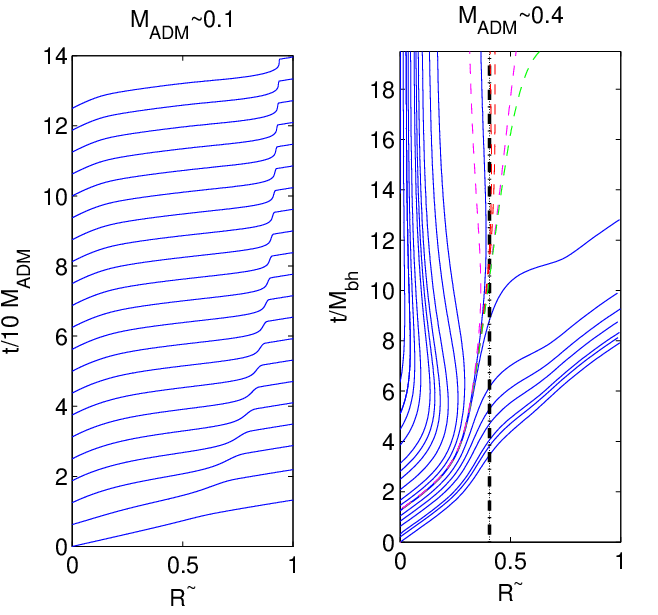
Event horizon. In contrast to the local definition (71) of the apparent horizon, the event horizon is a global concept: it is defined by outgoing null rays that neither escape to future null infinity, nor fall into the black-hole singularity. Clearly, this definition requires knowledge of the complete time evolution of the system, and hence, assuming a calculation that is carried out for a finite amount of coordinate (or proper) time, one cannot even in principle locate event horizons in numerically-generated spacetimes. However, when a spacetime approaches a stationary state, an approximate event horizon can be found. We employ the method of Libson et al [34] which is based on the observation that if one integrates the geodesic equation (73) backward in time, the event horizon becomes an attractor for geodesics that either escape to future null infinity or fall into the singularity at arbitrarily late times. We have found that in our simulations the event horizon is traced fairly well by the time development of the apparent horizon. Again this can be seen in Fig. 2, where the thin dashed lines show the trajectories obtained by integrating (73) backwards in time, and starting with several initial radii.

6 Results

For concreteness, we restrict our numerical experiments to the case of four-dimensional spacetimes, and take our matter source to be a real, massless scalar field. All of the results discussed here were generated using an initial scalar field profile of the Gaussian form (53), with fixed values $r_{0}=0$ and $\Delta=0.6$ , so that the scalar pulse is always initially centered at the origin. The overall amplitude, $\Phi_{0}$ , of the profile (53) is then used as a control parameter: variations of $\Phi_{0}$ produce varying “strengths” of initial data, and varying degrees of non-linearity in the ensuing evolution. In practice, the maximum value of $2m(t,r)/R(t,r)$ (where $R$ is the uncompactified areal radius) that is achieved in a given calculation is a useful indication of how strong-field the evolution becomes.

We use the above notion of initial data strength to loosely define three classes of solutions—within a given class we observe that the overall dynamics of each of the scalar and gravitational fields are similar. Specifically, we consider the following cases: (i) weak data, defined by $\Phi_{0}\lesssim 0.5$ , yielding $\max_{t,r}2m/R\simeq 0.08$ ; (ii) intermediate data, having $0.5\lesssim\Phi_{0}\lesssim 1.6$ , and $\max_{t,r}2m/R\simeq 0.25$ , and (iii) strong data, with $\Phi_{0}\gtrsim 1.6$ and $\max_{t,r}2m/R>0.25$ . While the first two cases describe weakly and mildly gravitating scalar pulses, respectively, which completely disperse in all instances, the strong data generates spacetimes in which black holes form, or almost form (i.e. near-critical evolution, see ([37])).

We have also found it useful to use the total ADM mass, $M_{\rm ADM}$ , of the spacetime—which can be computed at $t=0$ —to normalize certain numerical parameters. In particular, we set the parameters of the gauge driver (13,14) using $\xi_{1}={\xi_{10}}/M_{\rm ADM}^{2}$ , $\xi_{2}={\xi_{20}}/M_{\rm ADM}$ and $\xi_{3}={\xi_{30}}/M_{\rm ADM}^{2}$ , where the “bare” values, $\kappa_{0}$ , $\xi_{10}$ , $\xi_{20}$ and $\xi_{30}$ are generally held fixed as $\Phi_{0}$ is varied. Moreover, and as discussed in more detail below, we find that the accuracy of our results is improved if the constraint damping term asymptotically vanishes at large spatial distances. Accordingly, we typically multiplied $\kappa$ by the factor $2M_{\rm ADM}/R$ .

Because we use, at least in large part, a time-explicit finite difference scheme, we expect restrictions on the ratio $\lambda_{C}\equiv\Delta t/\Delta r$ (the Courant factor) that can be used while maintaining numerical stability. For the case of harmonic gauge, we found that values of $\lambda_{C}$ satisfying $0.01\lesssim\lambda_{C}\lesssim 0.8$ generated stable solutions with roughly constant accuracy, although somewhat stronger numerical dissipation was required to stabilize runs that used larger values of $\lambda_{C}$ in that interval. In the results discussed below we have typically taken $0.3\lesssim\lambda_{C}\lesssim 0.6$ for weak and intermediate data, and $0.1\lesssim\lambda_{C}\lesssim 0.2$ for the evolution of strong data. We further found that when any of the other gauge drivers were adopted, smaller Courant factors (relative to the harmonic case) were required. In those cases our results were generally computed using $0.05\lesssim\lambda_{C}\lesssim 0.1$ . Typically, in cases where $\lambda_{C}$ was taken too large, we observed amplification and dominance of numerical errors near the origin: this lead to high frequency oscillations and, eventually, to divergence of the numerical solution.

Another crucial numerical parameter is the Kreiss-Oliver dissipation factor, $\epsilon_{\rm KO}$ , which we generally set according to $0.1\lesssim\epsilon_{\rm KO}\lesssim 0.7$ . Finally, it is important to note that we found that optimal values of both $\lambda_{C}$ and $\epsilon_{\rm KO}$ were dependent on the spatial resolution: specifically, as $\Delta r\to 0$ somewhat smaller values of $\lambda_{C}$ , as well as larger values of $\epsilon_{\rm KO}$ were usually required. The lowest and highest resolution runs reported in this paper typically had $\Delta r=1/64$ and $\Delta r=1/8192$ , respectively: runs with $\Delta r=1/8192$ generally required $\lambda_{C}=0.05$ and $\epsilon_{KO}=0.7$ for stability.

Many of the coordinate conditions discussed and employed in this paper are characterized by several adjustable parameters, and we have by no means carried out exhaustive parameter space surveys in all cases in an attempt to optimize parameter settings. Rather, our more limited numerical experimentation indicates that with a certain amount of tuning of the parameters, it does seem possible, at least in principle, to simulate various interesting situations. Our intent here is chiefly to document the overall behavior of several gauge conditions as well as to explore some of the effects that specific parameters of the gauge drivers have on the evolution. Given this primary goal, we also defer most of our discussion of code convergence and accuracy to Sec. 6.4.

6.1 Weak data

In this section we consider the evolution of weak initial data for which $\Phi_{0}\lesssim 0.5$ , yielding $M_{\rm ADM}\lesssim 0.01$ and $\max_{t,r}2m/R\lesssim 0.08$ . In this case there is little interaction between the scalar and gravitational fields, the scalar pulse entirely disperses to infinity, and we find that essentially any of the gauge conditions described above can be used to produce long-term stable evolution. For this type of data we use $\epsilon_{\rm KO}\simeq 0.1$ for the Kreiss-Oliger dissipation parameter, finding that larger values have detrimental consequences for stability. However, even with dissipation and constraint damping, we find that numerical errors eventually do grow—on a time scale of order $t>10^{4}M_{\rm ADM}$ —and cause the code to crash.

We find that the effect of the constraint damping term depends on whether $\kappa$ is fixed or allowed to vary over the integration domain. For fixed $\kappa$ , it is essential to take $\kappa_{0}>0.01$ , otherwise high-frequency oscillations quickly ruin convergence. However, if the damping is too strong, instabilities are also triggered. In fact, we find that the optimal damping parameter is related to the typical scale over which the scalar field varies. For the Gaussian initial data that we consider, this scale is $\Delta$ , so we take $\kappa\simeq\Delta^{-1}$ . (This observation holds for intermediate strength data as well, as can be seen in Fig. 4.) On the other hand, when we take $\kappa=\kappa(r)$ , and specifically for the choice $\kappa=\kappa_{0}(2M_{\rm ADM}/R)$ mentioned previously, we find that the results are relatively insensitive to the value of $\kappa_{0}$ , provided $\kappa_{0}\lesssim 100\Delta^{-1}$ . For larger values of $\kappa_{0}$ instability is again usually observed.

Our experiments with the gauge drivers proposed by Lindblom et al, have focused on the specific Bona-Masso slicing condition for which $f(\alpha)=2/\alpha$ , corresponding to $1+\log$ slicing. However, for weak data, we find that other choices of $f$ (such as $f(\alpha)=2\alpha,\alpha^{2}$ and $10/\alpha^{2}$ , to list a few that we have tried) produce qualitatively similar results.

Considering the conditions that determine the shift, we find that the $\Gamma$ -driver condition performs somewhat better than $\Gamma$ -freezing, with the former allowing the evolution to be controlled for a longer amount of time. There was only mild dependence on the gauge-driver parameters, $\mu_{1,2},\eta_{1,2},q_{s},g_{n},\sigma$ and $\nu$ , provided they are all taken in the range $0.01$ – $10$ in units of $M_{\rm ADM}$ .

In order to assess the performance of the coordinate conditions in driving the source functions to the target functions, we first follow [18] and define the weighted $L_{2}$ -norm, $|Y|$ , of a function $Y$ as follows¹⁵¹⁵ 15 The integrals are evaluated on our fixed mesh using the trapezoidal rule. ,

|Y|=\left(\frac{\int e^{2S}Y^{2}{r}^{2}\sqrt{g_{rr}}d{r}}{\int e^{2S}{r}^{2}\sqrt{g_{rr}}d{r}}\right)^{1/2}.

(74)

A similar, if somewhat less smooth norm, which we also use here, can be defined as

|Y|_{L_{2}}=\frac{1}{N_{r}}\sqrt{\sum_{i=1}^{N_{r}}Y^{2}}.

(75)

Fig. 3 shows the weighted norms of the differences between the actual and target source functions from a typical weak-field simulation. It is evident from these plots that the drivers successfully drive the source functions $H_{\alpha}$ towards the target functions $F_{\alpha}$ as the evolution proceeds.

We now continue to discussions of the evolution of intermediate- and strong-field data, where the results are more sensitive to the specific driver used, as well as to the parameter settings for any given driver.

6.2 Intermediate data

Here we consider evolutions characterized by $0.5\lesssim\Phi_{0}\lesssim 1.6$ , where $M_{\rm ADM}\lesssim 0.1$ and $\max_{t,r}2m/R\lesssim 0.25$ . First, for this strength of data, we have found that the pure harmonic and GH gauges (43-44) perform comparably. With both choices, we are typically able to accurately trace the evolution of the initial data for times of the order of 100–600 $M_{\rm ADM}$ , with increasing resolution resulting in increased maximum evolution time.

The causal structure of the spacetime from a typical intermediate strength computation is displayed in the left panel of Fig. 2. We recall that in this figure the curves represent trajectories of outgoing null rays that are emitted at regular intervals (in coordinate time) from $r=0$ . As the evolution proceeds, the pulse, which is initially centered at the origin, disperses to infinity. The outgoing null rays are bent towards the origin by the presence of the matter and asymptotically become straight lines with unit slope in the $r-t$ plane. The position of the scattered pulse of scalar field can be traced through the location of the “ripple” in each curve, i.e. at the positions where the outgoing null geodesics suffer the most deflection.

We will discuss issues of code convergence and accuracy in more detail in Sec. 6.4. However, we note here that constraint norms, $|M_{\alpha}|_{L_{2}}$ , defined by (95) and computed, for example, using either (74) or (75) provide a basic indication of the accuracy of our numerical method. For the calculation depicted in Fig. 2 that uses a medium resolution, $\Delta r=1/1024$ , we find the initial norms $|M_{\alpha}|_{L_{2}}$ of order $10^{-4}$ , which for roughly the first half of the evolution then decrease to values of $10^{-5}$ – $10^{-6}$ . Thereafter we observe a slow increase in the size of the constraints although—except for the last few time steps before the code fails— $|M_{\alpha}|_{L_{2}}$ remain well below the $10^{-3}$ level. Moreover, we generally observe the expected quadratic convergence of $|M_{\alpha}|_{L_{2}}$ as the finite difference mesh is refined.

Another basic indication of numerical accuracy is provided by the the sum of the norms defined by (75) of the residuals of the dynamical equations, $|{\cal R}|_{L_{1}}=\sum_{Y}|{\cal R}_{Y}|$ , where ${\cal R}_{Y}$ is the FDA residual of the equation that governs the field $Y$ . Fig. 4 shows the behavior of $|{\cal R}|_{L_{2}}$ as a function of the damping parameter, $\kappa_{0}$ , for calculations with $N_{r}=513$ (moderate resolution), $\Phi_{0}=1.6$ , and where $\kappa=\kappa_{0}(2M_{\rm ADM}/R)$ . As already noted in the discussion of the weak field results, the sizes of the constraint and equation residuals tend to be minimized when $\kappa_{0}$ is comparable to the inverse of the typical length scale of the problem, i.e. to $\Delta^{-1}$ for our initially Gaussian data. This is apparent in the figure, which shows that for $\kappa_{0}=0.5/\Delta$ , the residuals remain on the order of $10^{-5}$ .

We next experiment with the Lindblom et al drivers, and find that while for $\Phi_{0}<0.7$ the dynamics of $H_{\alpha}$ and $F_{\alpha}$ is qualitatively similar to that in the weak field regime (shown in Fig. 3) and essentially independent of the parameters of the gauge drivers, for $\Phi_{0}>0.7$ the convergence of the source functions, $H_{\alpha}$ , towards the target sources, $F_{\alpha}$ , has stronger dependence on the parameter settings. The most pronounced feature in this regime is that the drivers succeed in forcing $H_{\alpha}\to F_{\alpha}$ only on the length-scale set by the parameter $\mu_{1}$ . In particular, when we start with initial data that has $H_{\alpha}=F_{\alpha}$ , we find that for large values of $\mu_{1}$ the source functions remain close to their targets for a a few tens of $M_{\rm ADM}$ , after which high-frequency oscillations destroy the matching. Conversely, starting from the same initial set up, but taking $\mu_{1}$ very small, we observe that the source functions quickly deviate from the targets and never approach them in the subsequent evolution.

Given this observation, and given that our Gaussian initial data generates an evolution characterized by a length scale, $\Delta$ , it is thus reasonable to take $\mu_{1}\simeq 1/\Delta$ in an attempt to enforce the desired gauge conditions on that scale. Results from such a computation are shown in Fig. 5, which displays the source and target functions, as well as their Fourier transforms, from the evolution of initial data with $\Phi_{0}=0.9$ . The calculations were performed using target slicing of the Bona-Masso type with $f(\alpha)=2/\alpha$ , and target $\Gamma$ -driver shift conditions with $\mu_{1}=1.3$ (recall that $\Delta=0.6$ for all of the computations described here). In addition, here, and for all of the results discussed in this section, we used $\mu_{2}=\eta=\eta_{2}=1$ , $q_{n}=q_{s}=0.5,\sigma=-1/3$ and $\nu=0.7$ . In contrast to the case of $\mu_{1}$ , we find that the calculations are not too sensitive to the settings of these parameters, so long as their values are all of order unity. In this simulation we begin with initial data satisfying $H_{\alpha}=F_{\alpha}$ . Within a few dynamical times the functions deviate, but as Fig. 5 demonstrates the functions are subsequently driven towards each other, when the source functions start resembling the targets on the spatial scales $1/\mu_{1}$ . Notice that the high-frequency spatial variations of the target $F^{\alpha}$ ’s are not replicated by the source functions. Similar behavior was originally observed in [18] for perturbations on a given background.

The manner in which the coordinate conditions evolve in time for this calculation is shown in Fig. 6, which depicts the norms of the functions $G_{t}$ and $G_{r}$ , defined by (19) or (20), and (24) or (27). As described in Sec. 3, enforcing a particular gauge is equivalent to driving these functions to zero. Since we begin with initial conditions in which the gauge is exactly fixed, the norms of $G_{t}$ and $G_{r}$ are initially zero. Then on a timescale of order several tens of $M_{\rm ADM}$ , the norms grow to some maximum value, after which they decrease slowly. The details depend on the particular coordinate choices, as well as on the settings of the driver parameters, but usually it is possible to drive the $L_{2}$ -norms of $G_{t}$ and $G_{r}$ to the level of about $0.01$ .

Although for smaller initial pulse amplitudes ( $\Phi_{0}\lesssim 1.0$ ) we managed to find parameters for the Lindblom et al drivers that asymptotically fix the desired gauges, we find that for larger amplitudes the effectiveness of the drivers degrades, and for $\Phi_{0}\gtrsim 1.0$ we could not find parameter settings that enforce any of the specific gauges. This does not necessarily mean that the code diverges: indeed, the evolution often proceeds, but the behavior of the source function is rather arbitrary. In this regime we find that the evolution systems based on the Lindblom et al drivers tend to be more dynamical and less stable than one that uses simple drivers such as (43).

6.3 Strong data and black hole formation

Increasing the initial amplitude, $\Phi_{0}$ , of the scalar pulse leads to increasingly strong curvature in the development of the initial data. As expected, above a critical value—in the current case, $\Phi_{0}\sim 2.15$ —black holes form, as signaled by the appearance of apparent horizons. We recall that we have already used the trajectories of outgoing null geodesics to schematically display the causal structure of a typical black hole geometry in the right panel of Fig. 2.

Our first set of numerical experiments in the strong-field regime compares subcritical evolution ( $\Phi_{0}\lesssim 2.15$ ) in pure harmonic coordinates to that in the generalized harmonic gauge given by (43). A generic feature of purely harmonic evolution in this case is a fairly quick collapse of the lapse function towards zero values near and at $r=0$ . As a result the evolution in the central region (where the pulse is concentrated) effectively freezes, and the scalar field remains present near $r=0$ even at late (coordinate) times. This is demonstrated in Fig. 7, which shows the evolution of central proper time

\tau(t)\equiv\int^{t}_{0}\alpha(t^{\prime},0)dt^{\prime},

(76)

as a function of the strength of the initial data.

On the other hand, and in accordance with the previous experience of Pretorius [9], we are able to use the generalized harmonic gauge condition (43) to inhibit the collapsing of the lapse. Specifically, we use $\alpha_{0}=1$ and $q=3$ in (43), and experiment with various values for $\xi_{1}$ and $\xi_{2}$ . In addition, motivated by an observation that we can more stably evolve subcritical data by gradually “turning-off” the gauge driving at late times, we actually replace $\xi_{1}$ and $\xi_{2}$ in (43) by $(\xi_{10}/M_{ADM}^{2})/(1+s\,t^{p})$ and $(\xi_{20}/M_{ADM})/(1+s\,t^{p})$ , respectively, where $p$ and $s$ are additional positive parameters. In practice, we have usually taken $p=1$ , leaving $s$ free to control the rate at which the gauge driving is disengaged.

Results from calculations with $\Phi_{0}=1.8$ ( $M_{\rm ADM}\simeq 0.125$ ) and using several sets of values for $\xi_{10}$ , $\xi_{20}$ and $s$ are shown in Fig. 8. The plots clearly show how judicious choice of the parameters can prevent the collapse of the lapse. Through experiments with various subcritical initial data sets we find that parameter values $1\lesssim\xi_{10}\lesssim 5$ and $0.5\lesssim\xi_{20}\lesssim 2$ produce good results. However, in order to keep the lapse from collapsing for initial data very close to criticality, we generally needed to increase both $\xi_{10}$ and $\xi_{20}$ by factors of up to 10, while simultaneously increasing $s$ (to values of order 50) and taking $p=2$ or $3$ . For instance, simulations that use $2049$ spatial grid points and the driver (43) with the parameters tuned to $\xi_{10}=50$ , $\xi_{20}=30$ , $s=36$ and $p=2$ allowed us to explore the dynamics of solutions with $\Phi_{0}=2.1465\pm 0.0005$ without encountering a collapsing lapse. Unfortunately this is not close enough to the threshold amplitude for us to be able to observe in detail the distinctive features of scaling and echoing known to appear in the near-critical regime of this model [37].

We end our discussion of subcritical strong-field evolution with two observations. First, we note that while we have investigated the use of dynamical conditions such as (44) for $H_{r}$ , the spatially harmonic choice, $H_{r}=0$ , is simpler to implement, and apparently more stable in this regime. Secondly, although we have experimented extensively with the Lindblom et al drivers in this context, we have not been able to find parameter settings that prevent coordinate pathologies (premature collapse of the lapse) from quickly developing for near-critical evolutions.

We now turn to the case of supercritical evolutions, which are characterized by the formation of black holes. As described in Sec. 5.3, we have implemented black hole excision techniques in our code: however, due to the strong singularity avoidance property of pure harmonic gauge, as well as the generalized harmonic modifications (43-44), we can also perform computations in which black holes form and are evolved for some amount of time, but where excision is not used.

For example, Fig. 9 shows metric functions from a calculation with $\Phi_{0}=3.0$ that uses pure harmonic gauge with no excision. We infer the formation of a black hole by the appearance of an apparent horizon, which at the end of the simulation is located at a compactified areal radius ${\tilde{R}}_{\rm AH}\simeq 0.4$ . We can then estimate the mass of the black hole at that time from the apparent horizon location: $M_{\rm BH}=0.5\,R_{\rm AH}\simeq 0.34$ , and note that the total ADM mass in this case is $M_{\rm ADM}\simeq 0.41$ . An apparent horizon is first detected at $t\simeq 1.25M_{\rm BH}$ and Fig. 9 displays the metric functions at two instants: $(i)$ $t\simeq 5M_{\rm BH}$ (dashed lines), and $(ii)$ $t\simeq 20M_{\rm BH}$ , which is shortly before the simulation crashes (solid lines). For this specific calculation we used $4097$ spatial grid points, and, at the time of the code crash, the values of the temporal component of the metric, $g_{tt}$ , near the origin are of order $10^{-15}$ (corresponding to lapse values of order $\sim 10^{-7}$ ). Despite the fact that all of the metric components displayed in Fig. 9 are tending towards zero at the origin at late times, the functions remain smooth and regular throughout the evolution. Fig. 10 plots central values for the Kretschmann scalar, $R_{\alpha\beta\gamma\delta}R^{\alpha\beta\gamma\delta}$ , as a function of time. The apparent divergence of this geometric quantity indicates the development of a curvature singularity.

We have found that the use of excision can somewhat extend the duration of our simulations of black hole spacetimes. For comparison, a run with the same parameters enumerated above, but employing excision, lasted for as long as $\sim 60M_{\rm BH}$ . We recall that our simple approach to excision has been described in Sec. 5.3, and note that in practice we have typically chosen the excision radius, $r_{\rm EX}$ , to satisfy $r_{\rm EX}\leq 0.4r_{\rm AH}$ . The rest of the results described in this section were obtained in simulations with excision.

Although we are able to avoid the central singularity using excision, it is clear from our calculations that the harmonic coordinate system continues to evolve in a highly non-trivial manner after excision is initiated. This dynamics in the coordinates causes, or is at least associated with, two main problems. First, the resulting coordinate system does not approach a stationary state: in particular, the coordinate position of the apparent horizon evolves with time. Specifically, after formation, the horizon expands outwards and consumes most of the numerical grid. Eventually then, the portion of the spacetime outside the horizon—which we recall extends to spatial infinity due to our use of a compactified coordinate system—is represented by only a small portion of the initial lattice. Consequently, numerical errors that arise near the outer boundary dominate the late stages of the evolution. The second problem is that the lapse continues to decrease in the vicinity of $r_{\rm EX}$ , and becomes very small. In this situation truncation errors in quantities near $r_{\rm EX}$ occasionally cause the computation of non-positive values for the lapse, which immediately leads to code failure. Both of these problems can be somewhat mitigated by increasing the numerical resolution. In harmonic gauge, we were able to simulate the formation of a black hole and resolve it for about $t\simeq 70M_{\rm BH}$ using our finest resolution, $N_{r}=8193$ . However, given these difficulties induced by the late-time dynamics when using harmonic coordinates, it is quite natural to try to use the coordinate freedom provided by the various gauge drivers discussed above to a) attempt to minimize the time development of the lapse following the formation of an apparent horizon, and/or b) implement a non-trivial shift vector with an aim to minimize the outward expansion of $r_{\rm AH}$ at late times when there is very little matter falling into the black hole. We thus now summarize our experimentation with several driver conditions that was focused on realizing these ideas.

As we have already mentioned, one of the main motivations for Pretorius’ development of the driver condition (43) was to keep the lapse from collapsing in the vicinity of horizons [9]. Following that work then, we first used (43) to fix the time slicing, while maintaining harmonic spatial coordinates ( $H_{r}=0$ ). However, in contrast to the results reported in [9] (which we note were performed in three spatial dimensions using Cartesian coordinates), we found the evolution in this case to be significantly less stable than purely harmonic evolution. For example, even a small value of $\xi_{1}$ of order $0.01M_{\rm BH}^{2}$ resulted in a code crash at a time about a factor of two earlier than for the harmonic case, irrespective of the value of the friction parameter, $\xi_{2}$ .

We next used harmonic slicing, $H_{t}=0$ , while evolving $H_{r}$ using the driver (44). Here, we found a modest amount of improvement over the purely harmonic case, in that the “grid-sucking” phenomenon described above was slowed, with an accompanying reduction in the development of numerical error in the outer, low-resolution region. For example, the duration of the evolution of $\Phi_{0}=3$ initial data with $\xi_{20},\xi_{30}\sim{\cal O}(10)M_{\rm BH}\times(1+5t^{2})^{-1}$ , increases by approximately $20\%$ compared to the corresponding harmonic evolution.

Interestingly, we obtained even better results using certain versions of the Lindblom et al gauge drivers. For the strong-field, supercritical calculations described here, we found that versions of the drivers that use the simple scalar operator (47) performed better than those that used (46). Moreover, we found that drivers based on the Bona-Masso slicing and $\Gamma$ -driver shift conditions (with suitably tuned parameters) gave the best results, and for convenience will hereafter refer to this specific choice as BMGD. In particular, relative to other driver choices, this combination minimized—but unfortunately did not completely eliminate—the outward drift of $r_{\rm AH}$ . Our best configuration allowed for accurate simulation of black hole spacetimes for about $100M_{\rm BH}$ following the formation of an apparent horizon. After that time, code accuracy typically degraded, numerical errors near the excision became dominant, and a late-time instability ensued. Based on our experiments, it remains unclear whether specific parameter choices for the drivers exist that would totally eliminate the drift of the coordinate position of the apparent horizon and, even more importantly, the disastrous collapse of the lapse inside the horizon.

We now proceed to some details concerning our experience with the BMGD version of the Lindblom et al coordinate conditions. The parameters $q_{n}$ and $q_{s}$ that appear in the driver definitions—see equations (21,28)—control the relative weight that the gauge functions, $G^{\alpha}$ , have in forming the target sources, $F^{\alpha}$ . We also recall that the $G^{\alpha}$ vanish when the specific gauge to which they correspond is attained. We found it crucial not to choose $q_{n}$ too large: usually values in the range $0.01-0.1$ resulted in the most stable evolutions, and would eventually lead to the desired behavior, $H^{\alpha}\rightarrow F^{\alpha}$ and $G\rightarrow 0$ . Our implementation was less sensitive to the value of $q_{s}$ , with results of comparable accuracy and stability being attained for $g_{s}$ in the range $0.01-10$ .

Having determined good values for $q_{n}$ and $q_{s}$ , we found through further experimentation that stability is improved when the parameters $\mu_{1},\mu_{2}$ and $\eta$ are multiplied by a decay factor $2M_{\rm ADM}/R$ in the region external to the horizon. This localizes the effect of the coordinate drivers to the near-horizon region, while producing a smooth blend to harmonic coordinates at spatial infinity. In addition, and in analogy to what we did for the subcritical calculations in generalized harmonic coordinates described earlier in this section, we further scale $\mu_{1}$ , $\mu_{2}$ and $\eta$ , as well as $q_{n}$ by $1/(1+st^{p})$ . Here, $s$ and $p$ are again positive tunable quantities—we typically used $p=2$ and $s=5$ —that result in a late-time decay of the scaled driver parameters. We note that the values quoted below generally refer to “bare” values for parameters, with the additional scaling factors being implied.

Fig. 11 shows the time development of the deviation between the target and actual source functions, $F_{\alpha}$ and $H_{\alpha}$ , respectively, as well as the gauge functions, $G^{\alpha}$ , for a typical BMGD calculation. The computation was performed with $\mu_{1}=4\simeq 1/M_{\rm BH}$ , $\mu_{2}=\eta=\eta_{2}=10$ $\nu=1,\sigma=-1/3,q_{n}=0.1$ and $q_{s}=1$ . The behavior of the two upper plots in the figure reflect the fact that the $H^{\alpha}$ tend to the target source functions soon after an apparent horizon forms. Detailed examination of the data reveals that the match between the target and actual source functions is good throughout the entire domain for a certain amount of time following horizon formation. At late times the level of global agreement degrades, due to large scale variations in the $F^{\alpha}$ induced by the portion of the scalar field that is scattered to infinity. Despite this, we still find that actual sources accurately match the targets on the scale defined by $\mu_{1}^{-1}\simeq R_{\rm AH}$ (not shown). The plots of the $L_{2}$ norms of the gauge functions, $G^{\alpha}$ , shown in the bottom half of the figure, reveal a steady decrease in time, signaling that the desired gauge is being approached asymptotically.

Our investigations of versions of the drivers using target functions corresponding to “static” gauges, such as maximal slicing and $\Gamma$ -freezing, were unsuccessful in the sense that we were not able to find parameter settings that resulted in $G^{\alpha}\rightarrow 0$ as $t\to\infty$ . Interestingly, however, we found that black holes could nonetheless be simulated using these conditions, with observed stability properties similar to those obtained using “dynamic” gauge conditions such as BMGD. This indicates that, at least for the type of initial data considered here, the stability of the drivers (15,16) does not strongly depend on the target gauge.

Finally we note that the use of an appropriate amount of constraint damping is important for computations in which black holes form. Fig. 12 shows the behavior of the sum of the $L_{2}$ -norms of the constraints, (75), in a sample run with $N_{r}=4097$ and using various values for the damping parameter, $\kappa_{0}$ . The plots provide clear evidence that the level of constraint maintenance (as well as the maximum simulation time) is optimized for $\kappa_{0}\simeq M_{\rm BH}^{-1}$ . Values of $\kappa_{0}$ significantly larger than the optimal value produce rapid code crashes, while those that are significantly smaller lead to poorer preservation of the constraints.

6.4 Code accuracy, convergence and constraints

In this section we briefly discuss some of the technical issues relating to the basic performance of our numerical code, including resolution requirements and checks of convergence.

Not surprisingly, we find that the minimum discretization scale required to produce an acceptable evolution (for fixed choice of coordinate conditions) depends on the strength of the initial data. For example, in the case of weak and intermediate initial data, as defined previously, even a modest lattice size of $N_{r}=65$ is enough to allow for long-time evolution. However, for stronger data, meshes sizes of at least $N_{r}=257$ are required. Additionally, our code cannot evolve strong-field data for arbitrary amounts of coordinate time: generically, numerical problems develop that lead to a code crash on the order of 10-100 $M_{\rm ADM}$ , and the precise lifetime of the simulation is dependent on the strength of the initial data, the resolution, and the details of the coordinate conditions.

Much of the build-up of error that eventually leads to code failure, especially in subcritical simulations, can be traced to the use of spatial compactification. In all of our calculations, there is outflux of scalar field to spatial infinity, and as the scalar radiation propagates to large distances it becomes more poorly resolved on the mesh, which has uniform spacing in the compactified radial coordinate. Untreated, this will lead to spurious reflection of the waves which will corrupt the interior solution, so we add Kreiss-Oliger dissipation to explicitly damp the radiation when its wavelength becomes of order the mesh scale. Although this damping is imperfect, we find that increasing the resolution is effective in extending the lifetime of our evolutions. As a specific example, for a calculation which forms a black hole of size ${\tilde{R}}_{\rm BH}\simeq 0.6$ , and that uses BMGD coordinate conditions and excision, a grid with $N_{r}=4097$ is sufficient to keep the reflections small during all stages of the evolution until $t\simeq 100M_{\rm BH}$ . Thereafter, an instability appears near $r_{\rm EX}$ and leads to a code crash.

A crucial test of any finite difference code for the solution of a system of partial differential equations involves the investigation of the convergence of the generated numerical solutions as a function of resolution. We perform straightforward convergence tests based on the assumption (originally due to Richardson [39]) that for any of the unknown functions, $Y(t,r)$ , appearing in our differential system, the corresponding finite difference quantity, $Y_{h}(t,r)$ in the limit $h\to 0$ admits an asymptotic expansion of the form

Y_{h}(t,r)=Y(t,r)+h^{p}e_{p}(t,r)+\cdots

(77)

where $h$ is the discretization scale, $e_{p}(t,r)$ is an $h$ -independent error function with smoothness comparable to $Y(t,r)$ , and $p$ is an integer which defines the order of convergence of the scheme. Following standard practice, we consider sequences of three calculations performed with identical initial conditions, but with varying resolutions, $h$ , $h/2$ and $h/4$ . We then form the differences, $c_{1}=Y_{h}-Y_{h/2}$ and $c_{2}=Y_{h/2}-Y_{h/4}$ , and compute

\log_{2}\left(\frac{c_{1}}{c_{2}}\right)\approx p.

(78)

Fig. 13 shows the results of such a convergence test for the scalar field, $\Phi(t,r)$ , from computations in pure harmonic coordinates, and with initial data defined by $\Phi_{0}\simeq 0.55$ . The plot provides evidence for the expected second order convergence ( $p=2$ ) of $\Phi_{h}$ , and similar results are observed for the other dynamical variables. We note, however, that there is an obvious degradation of convergence at the highest resolutions used: this issue has not been resolved, but may be related to the time-stepping iteration.

As discussed in Sec. 5.1, in the cases where the Lindblom et al drivers were used to evolve the source functions, we used an implicit Euler method to integrate the corresponding finite difference equations. Since that method is only first-order accurate in time, the convergence of the overall scheme in only expected to be first order, and this was in fact observed.

Finally, since we have implemented a free evolution scheme [38], we can also assess the convergence of our numerical solutions by monitoring discrete versions of the Hamiltonian and momentum constraints, $M_{t}$ and $M_{r}$ , respectively. As usual, these constraints are defined by contracting the Einstein equations with the unit normal vector to the $t={\rm const.}$ hypersurfaces, i.e. $M_{\alpha}\equiv n^{\alpha}(G_{\alpha\beta}-T_{\alpha\beta})$ , where $G_{\alpha\beta}$ is the Einstein tensor. In order to estimate how well the constraints are satisfied, we discretize them to second order, and then compute their $L_{2}$ -norms, as defined by (75), at each time step. Fig. 14 shows a typical plot of the results for weak initial data ( $M_{\rm ADM}\simeq 0.01$ ) evolved with harmonic coordinates. It is clear from the figure that the constraint violations remain quite small during the evolution, and that—modulo the previous remark concerning an apparent problem at higher resolutions—the constraints are increasingly well satisfied as $h\to 0$ .

7 Conclusions

We have presented a generalized harmonic formulation of the Einstein equations for spherically symmetric $D$ -dimensional spacetimes. Since it is natural to choose coordinates in which the symmetries of the geometry are explicit, we have adopted the usual spherical coordinates. This results in a coordinate singularity at the origin, $r=0$ . While at the continuum level the equations of motion maintain regularity of a solution which is initially smooth at the origin, extra care must be exercised so that this property is reflected in discrete numerical calculations. We have thus described a procedure to ensure that the origin remains regular in numerical calculations, while preserving the hyperbolicity of the evolution system.

We have investigated the resulting GH system in the context of fully non-linear gravitational collapse. To this end we introduced a real, massless scalar field, and have used the specification of the initial scalar field profile to control the ensuing strength of the gravitational interaction. The dynamics that we have considered range from the dispersion of weak pulses to the collapse of strong pulses that lead to black hole formation. A key aspect of our numerical approach was the use of radial compactification which, in conjunction with sufficient dissipation, provided a viable alternative to the truncation of the spatial domain and the use of approximate outer boundary conditions. Another ingredient of our methodology that was vital for long-term stability of the numerical calculations was the addition of constraint-damping terms to the evolution equations.

Our studies of evolutions using several coordinate drivers lead us to conclude that, in spherical geometries, the gauge drivers discussed in [9, 10, 18, 19] are less effective relative to the $3+1$ simulations that use Cartesian coordinates, and it would be very interesting to understand this issue in more detail. Nevertheless, we found that with a certain amount of parameter tuning many interesting situations could be successfully simulated with drivers that have been proposed in the literature. Perhaps not surprisingly, depending on the situation certain drivers performed better than others, leading to longer and/or more accurate simulations. Specifically, the dynamics of weakly gravitating dispersing pulses could be simulated using any of the considered coordinate choices; however the pure harmonic gauge arguably provided the cleanest and the simplest choice. For strong-field data, variations in the performance of the various drivers were more apparent. In particular, for strong but subcritical pulses, the harmonic gauge quickly lead to coordinate pathologies, signaled by a collapsing lapse, but this behavior could be partially ameliorated by using one the drivers given by (13) and (14). The driver (15) could also be used to evolve strong-field data in some regimes, but the target coordinates which it is designed to asymptotically enforce, were not achieved, at least not for the range of the parameters that we explored in this work.

For the case of strong-field, supercritical calculations (i.e. those for which black holes form), we found that pure harmonic coordinates could still be of use. In the simulations that used excision, it was possible to evolve black holes for as long as a few tens of dynamical times. However, the coordinate system remained fairly dynamic even at late times, leading to collapse of the lapse near the excision surface on one hand, and to the outwards expansion of the coordinate position of the horizon on the other. We were able to use driver conditions to moderate the time-dependence, with the best results being obtained through the use of the drivers (15) with the Bona-Masso target slicing and the $\Gamma$ -driven target shift. It would be very interesting to find out whether or not parameters and target gauges exist that not only slow down the time-dependence of the coordinates at late times, but completely eliminate it.

One of the main goals of this work was to achieve a better understanding of the generalized harmonic approach as applied to highly symmetric spacetimes, and to prepare ground for an exploration of various gravitational phenomena in axisymmetry using an analogous formalism. We expect that the insights gained from our experiments in spherical symmetry will also prove useful in the axially symmetric case. In particular, coordinates that are adapted to the axial symmetry are again formally singular on the axis, and the equations of motion will need to be regularized there. However, the same regularization described above for spherical symmetry can be readily extended to that case. This allows for a regular hyperbolic formulation in axial symmetry, which will be discussed in a subsequent publication [32].

Acknowledgments.

We would like to thank Frans Pretorius for interesting and useful discussions, and for tips on the use of the PAMR/AMRD software [40]. MWC also gratefully acknowledges the financial research support of NSERC and CIFAR, and thanks the MPI-AEI for hospitality and support while part of this work was carried out.

Appendix A Asymptotically AdS spacetime

Here we analyze the asymptotics of $AdS$ spacetime, and discuss a convenient metric ansatz as well as a normalization of the source functions.

The $AdS_{D}$ background can be written in the form,

ds^{2}=-(1+\rho^{2}/\ell^{2})d\tau^{2}+d\rho^{2}/(1+\rho^{2}/\ell^{2})+\rho^{2}\,d\Omega_{n}^{2},

(79)

where $\ell$ is the AdS curvature scale. In our model (30) we reproduce asymptotically AdS spacetime by letting $V(0)=\Lambda<0$ that defines $\ell^{2}=-(D-1)(D-2)/\Lambda$ .

One of the properties of the AdS space is that its asymptotic boundary is time-like: in fact, it takes only a finite time for a light signal to propagate to the boundary. Hence, in numerical implementations, correct treatment of boundary conditions at spatial infinity is crucial. To this end it is useful to transform to conformal coordinates,

\rho=\ell\tan(r/\ell),~~~~\tau=t,

(80)

in which the AdS metric becomes

ds^{2}=-\cos^{-2}\left(r/\ell\right)\left(dt^{2}-dr^{2}\right)+\ell^{2}\,\tan^{2}(r/\ell)\,d\Omega^{2}_{n}.

(81)

We note that the entire space has finite extent $r\in\left[0,\pi\ell/2\right]$ in these coordinates, but that the metric is singular at spatial infinity, $r=\pi\ell/2$ .

A convenient metric ansatz for evolution using the generalized harmonic approach explicitly factors out the background and is given by

ds^{2}=-cos^{-2}\left(r/\ell\right)g_{tt}\,\left(dt^{2}-dr^{2}\right)+2g_{tr}dtdr+\ell^{2}\,\tan^{2}(r/\ell)\,e^{2\,S}d\Omega^{2}_{n}.

(82)

In this case the asymptotic behavior of the fields $g_{ab}$ is regular, $g_{ab}\rightarrow\eta_{ab}$ and $S\rightarrow 0$ .

The source function obtained from (4) does not vanish in spherical coordinates even in pure AdS where it becomes

H^{AdS}_{\mu}=\left(0,(n/\rho)[1+((n+2)/n)(\rho^{2}/\ell^{2})]/[1+\rho^{2}/\ell^{2}],(n-1)\,\cot\theta_{1},\dots,\cot\theta_{n-1},0\right),

(83)

and where $\rho$ is given in (80). In analogy with the asymptotically flat case, we subtract a background contribution, which is singular at $\rho=0$ , by writing $H_{\alpha}=H_{\alpha}+H_{\alpha}^{AdS}$ , and then use the regular source functions

H_{\alpha}=\left(H_{t}(t,r),H_{r}(t,r)+\frac{n}{\rho}\frac{1+\frac{n+2}{n}\frac{\rho^{2}}{\ell^{2}}}{1+\frac{\rho^{2}}{\ell^{2}}},(n-1)\cot\theta_{1},(n-2)\,\cot\theta_{2},\dots,\cot\theta_{n-1},0\right).

(84)

Appendix B Explicit form of the equations

We define $g_{2}\equiv g_{tt}\,g_{rr}-g_{tr}^{2}$ , to be the determinant of the 2-metric $g_{ab}$ , in (35). The complex scalar field is decomposed as $\Phi=\phi_{r}+i\,\phi_{i}$ .

The Christoffel symbols and the trace of the extrinsic curvature are given by

$\displaystyle\Gamma_{t}$	$\displaystyle=$	$\displaystyle\left(g_{tt}\,g_{tr}^{\prime}-g_{tr}\,g_{tt}^{\prime}-{1\over 2}g_{tt}\dot{g}_{tr}+{1\over 2}g_{rr}\dot{g}_{tt}-n\,g_{2}\,\dot{S}\right)/g_{2}$
$\displaystyle\Gamma_{r}$	$\displaystyle=$	$\displaystyle-\frac{n}{r}+\left({1\over 2}g_{tt}\,g_{rr}^{\prime}-{1\over 2}g_{rr}\,g_{tt}^{\prime}-g_{tr}\dot{g}_{rr}+g_{rr}\,\dot{g}_{tr}-n\,g_{2}\,S^{\prime}\right)/g_{2}$	(85)
$\displaystyle K$	$\displaystyle=$	$\displaystyle\alpha\left(-\frac{n\,g_{tr}}{r}+\frac{g_{tr}}{ng_{rr}}g_{rr}^{\prime}-g_{tr}^{\prime}-2g_{tr}\,S^{\prime}+{1\over 2}\,\dot{g}_{rr}+n\,g_{rr}\,\dot{S}\right)/g_{2},$	(86)

The generalized harmonic equations (40,41) in $4D$ become

$\displaystyle R_{tt}-C_{(t;t)}-\bar{T}_{tt}$	$\displaystyle=$	(87)
	$\displaystyle-\frac{1}{4}\left(\dot{g}_{rr}\right)^{2}(g^{rr})^{2}+g_{tr}^{\prime}\dot{g}_{rr}(g^{rr})^{2}+{g^{tt}}\left(\dot{g}_{tr}\right)^{2}{g^{rr}}-\frac{1}{2}g_{tt}^{\prime\prime}{g^{rr}}+{g^{tr}}g_{tt}^{\prime}\dot{g}_{rr}{g^{rr}}+$
	$\displaystyle 4{g^{tr}}g_{tr}^{\prime}\dot{g}_{tr}{g^{rr}}+\frac{\left(g_{tt}^{\prime}\right)^{2}}{2{g_{2}}}+\frac{3}{4}(g^{tt})^{2}\left(\dot{g}_{tt}\right)^{2}-\left(\dot{\phi}_{i}\right)^{2}-\left(\dot{\phi}_{r}\right)^{2}-2\left(\dot{S}\right)^{2}+$
	$\displaystyle\left(\frac{{g_{tr}}{H_{t}}-{g_{tt}}{H_{r}}}{2{g_{2}}}-\frac{{g_{tt}}}{{g_{2}}r}\right)g_{tt}^{\prime}+\left(\frac{2{g_{tt}}}{{g_{2}}r}+\frac{{g_{tt}}{H_{r}}-{g_{tr}}{H_{t}}}{{g_{2}}}\right)\dot{g}_{tr}+$
	$\displaystyle\left(\frac{{g_{rr}}{H_{t}}-{g_{tr}}{H_{r}}}{2{g_{2}}}-\frac{{g_{tr}}}{{g_{2}}r}\right)\dot{g}_{tt}+(g^{tr})^{2}g_{tr}^{\prime}\dot{g}_{tt}+2{g^{tr}}{g^{tt}}g_{tt}^{\prime}\dot{g}_{tt}+\frac{1}{2}(g^{tr})^{2}\dot{g}_{rr}\dot{g}_{tt}+$
	$\displaystyle 2{g^{tr}}{g^{tt}}\dot{g}_{tr}\dot{g}_{tt}-\dot{H}_{t}-{g^{tr}}\dot{g}_{tt}^{\prime}-\frac{1}{2}{g^{tt}}\ddot{g}_{tt}-{g_{tt}}V+2(g^{tr})^{2}g_{tt}^{\prime}\dot{g}_{tr},$

$\displaystyle R_{tr}-C_{(t;r)}-\bar{T}_{tr}$	$\displaystyle=$	(88)
	$\displaystyle\frac{1}{2}g_{rr}^{\prime}g_{tr}^{\prime}(g^{rr})^{2}+\frac{1}{2}g_{rr}^{\prime}\dot{g}_{rr}(g^{rr})^{2}+{g^{tr}}\left(g_{tr}^{\prime}\right)^{2}{g^{rr}}+\frac{1}{2}{g^{tr}}\left(\dot{g}_{rr}\right)^{2}{g^{rr}}+$
	$\displaystyle\frac{1}{2}{g^{tr}}g_{rr}^{\prime}g_{tt}^{\prime}{g^{rr}}-\frac{1}{2}g_{tr}^{\prime\prime}{g^{rr}}+{g^{tr}}g_{rr}^{\prime}\dot{g}_{tr}{g^{rr}}+\frac{1}{2}{g^{tr}}{g^{tt}}\left(g_{tt}^{\prime}\right)^{2}+{g^{tr}}{g^{tt}}\left(\dot{g}_{tr}\right)^{2}-$
	$\displaystyle{g_{tr}}V+\left(\frac{{g_{rr}}{H_{t}}-{g_{tr}}{H_{r}}}{2{g_{2}}}-\frac{{g_{tr}}}{{g_{2}}r}\right)g_{tt}^{\prime}+\left(\frac{(g^{tr})^{2}}{2}+{g^{rr}}{g^{tt}}\right)g_{tr}^{\prime}g_{tt}^{\prime}-\frac{1}{2}H_{t}^{\prime}+$
	$\displaystyle\left(\frac{{g_{tt}}}{{g_{2}}r}+\frac{{g_{tt}}{H_{r}}-{g_{tr}}{H_{t}}}{2{g_{2}}}\right)\dot{g}_{rr}+\frac{1}{4}\left((g^{tr})^{2}-2{g^{rr}}{g^{tt}}\right)g_{tt}^{\prime}\dot{g}_{rr}+2{g^{tr}}^{2}g_{tr}^{\prime}\dot{g}_{tr}+$
	$\displaystyle\left(\frac{(g^{tr})^{2}}{2}+{g^{rr}}{g^{tt}}\right)\dot{g}_{rr}\dot{g}_{tr}+\frac{3}{4}(g^{tr})^{2}g_{rr}^{\prime}\dot{g}_{tt}+{g^{tr}}{g^{tt}}g_{tr}^{\prime}\dot{g}_{tt}+\frac{1}{2}(g^{tt})^{2}g_{tt}^{\prime}\dot{g}_{tt}+$
	$\displaystyle\frac{1}{2}(g^{tt})^{2}\dot{g}_{tr}\dot{g}_{tt}-\frac{1}{2}\dot{H}_{r}-2\phi_{i}^{\prime}\dot{\phi}_{i}-2\phi_{r}^{\prime}\dot{\phi}_{r}-4S^{\prime}\dot{S}-\frac{2\dot{S}}{r}-{g^{tr}}\dot{g}_{tr}^{\prime}-\frac{1}{2}{g^{tt}}\ddot{g}_{tr}+$
	$\displaystyle\frac{1}{2}{g^{tr}}{g^{tt}}\dot{g}_{rr}\dot{g}_{tt},$

$\displaystyle R_{rr}-C_{(r;r)}-\bar{T}_{rr}$	$\displaystyle=$	(89)
	$\displaystyle\frac{1}{2}g_{rr}^{\prime}g_{tt}^{\prime}(g^{tr})^{2}+2g_{tr}^{\prime}\dot{g}_{rr}(g^{tr})^{2}+g_{rr}^{\prime}\dot{g}_{tr}(g^{tr})^{2}+2{g^{rr}}g_{rr}^{\prime}g_{tr}^{\prime}{g^{tr}}+2{g^{rr}}g_{rr}^{\prime}\dot{g}_{rr}{g^{tr}}+$
	$\displaystyle{g^{tt}}g_{tt}^{\prime}\dot{g}_{rr}{g^{tr}}+4{g^{tt}}g_{tr}^{\prime}\dot{g}_{tr}{g^{tr}}-\dot{g}_{rr}^{\prime}{g^{tr}}+\frac{3}{4}(g^{rr})^{2}\left(g_{rr}^{\prime}\right)^{2}+{g^{rr}}{g^{tt}}\left(g_{tr}^{\prime}\right)^{2}-$
	$\displaystyle\left(\phi_{i}^{\prime}\right)^{2}-\left(\phi_{r}^{\prime}\right)^{2}-2\left(S^{\prime}\right)^{2}+\frac{\left(\dot{g}_{rr}\right)^{2}}{2{g_{2}}}-{g_{rr}}V+\left(\frac{{g_{tt}}}{{g_{2}}r}+\frac{{g_{tt}}{H_{r}}-{g_{tr}}{H_{t}}}{2{g_{2}}}\right)g_{rr}^{\prime}+$
	$\displaystyle\left(\frac{{g_{rr}}{H_{t}}-{g_{tr}}{H_{r}}}{{g_{2}}}-\frac{2{g_{tr}}}{{g_{2}}r}\right)g_{tr}^{\prime}-H_{r}^{\prime}-\frac{4S^{\prime}}{r}+\left(\frac{{g_{tr}}}{{g_{2}}r}+\frac{{g_{tr}}{H_{r}}-{g_{rr}}{H_{t}}}{2{g_{2}}}\right)\dot{g}_{rr}+$
	$\displaystyle({g^{tt}})^{2}g_{tt}^{\prime}\dot{g}_{tr}-\frac{1}{4}(g^{tt})^{2}\left(g_{tt}^{\prime}\right)^{2}-\frac{1}{2}{g^{tt}}\ddot{g}_{rr}-\frac{1}{2}{g^{rr}}g_{rr}^{\prime\prime},$

$\displaystyle R_{\theta\theta}-C_{(\theta;\theta)}-\bar{T}_{\theta\theta}$	$\displaystyle=$	(90)
	$\displaystyle-\frac{2S^{\prime}{g_{tt}}}{{g_{2}}r}-\frac{{g_{tt}}}{{g_{2}}r^{2}}+\frac{e^{-2S}}{r^{2}}-V+\frac{2{g_{tr}}\dot{S}}{{g_{2}}r}+{H_{t}}\left(\frac{S^{\prime}{g_{tr}}}{{g_{2}}}+\frac{{g_{tr}}}{{g_{2}}r}-\frac{{g_{rr}}\dot{S}}{{g_{2}}}\right)+$
	$\displaystyle{H_{r}}\left(-\frac{S^{\prime}{g_{tt}}}{{g_{2}}}-\frac{{g_{tt}}}{{g_{2}}r}+\frac{{g_{tr}}\dot{S}}{{g_{2}}}\right)-2{g^{tr}}\dot{S}^{\prime}-{g^{tt}}\ddot{S}-{g^{rr}}S^{\prime\prime}.$

Written in full, the constraint damping terms, $Z_{\mu\nu}=\kappa\left(n_{(\mu}{\cal C}_{\nu)}-{1\over 2}g_{\mu\nu}\,n^{\beta}\,{\cal C}_{\beta}\right)$ , that we subtract from the above equations to form (9), are

$\displaystyle Z_{tt}$	$\displaystyle=$		(91)
		$\displaystyle\frac{\alpha\kappa}{g_{2}}\Big[-\frac{{g_{tr}}g_{rr}^{\prime}{g_{tt}}^{2}}{4\ {g_{2}}}+\frac{{g_{rr}}\dot{g}_{rr}{g_{tt}}^{2}}{4{g_{2}}}-\frac{{g_{tr}}{H_{r}}{\ g_{tt}}}{2}-\frac{\left({g_{rr}}{g_{tt}}-2{g_{tr}}^{2}\right)g_{tr}^{\prime}{g_{tt}}}{2{g_{2}}}+$
		$\displaystyle{\ g_{tr}}S^{\prime}{g_{tt}}-\frac{{g_{rr}}{g_{tr}}\dot{g}_{tr}{g_{tt}}}{2\ {g_{2}}}+\left({g_{tr}}^{2}-\frac{{g_{rr}}{g_{tt}}}{2}\right){H_{t}}+\frac{{g_{tr}}\left(3\ {g_{rr}}{g_{tt}}-4{g_{tr}}^{2}\right)g_{tt}^{\prime}}{4{g_{2}}}-$
		$\displaystyle\frac{{g_{rr}}\left({g_{rr}}\ {g_{tt}}-2{g_{tr}}^{2}\right)\dot{g}_{tt}}{4{g_{2}}}+\left({g_{rr}}{g_{tt}}-2{g_{tr}}^{2}\right)\ \dot{S}\Big],$

$\displaystyle Z_{tr}$	$\displaystyle=$		(92)
		$\displaystyle\frac{\alpha\kappa}{g_{2}}\Big[-\frac{{g_{tt}}\dot{g}_{tr}{g_{rr}}^{2}}{2\ {g_{2}}}+\frac{{g_{tr}}\dot{g}_{tt}{g_{rr}}^{2}}{4{g_{2}}}-\frac{{g_{tt}}{H_{r}}{\ g_{rr}}}{2}+\frac{{g_{tr}}{H_{t}}{g_{rr}}}{2}-\frac{{g_{tt}}^{2}g_{rr}^{\prime}\ {g_{rr}}}{4{g_{2}}}+$
		$\displaystyle\frac{{g_{tr}}{g_{tt}}g_{tr}^{\prime}{g_{rr}}}{2{g_{2}}}+\frac{\left({\ g_{rr}}{g_{tt}}-2{g_{tr}}^{2}\right)g_{tt}^{\prime}{g_{rr}}}{4{g_{2}}}+{g_{tt}}S^{\prime}\ {g_{rr}}+\frac{{g_{tr}}{g_{tt}}\dot{g}_{rr}{g_{rr}}}{4{g_{2}}}-{g_{tr}}\dot{S}{\ g_{rr}}\Big],$

$\displaystyle Z_{rr}$	$\displaystyle=$		(93)
		$\displaystyle\frac{\alpha\kappa}{g_{2}}\Big(-\frac{{g_{tt}}\dot{g}_{tr}{g_{rr}}^{2}}{2\ {g_{2}}}+\frac{{g_{tr}}\dot{g}_{tt}{g_{rr}}^{2}}{4{g_{2}}}-\frac{{g_{tt}}{H_{r}}{\ g_{rr}}}{2}+\frac{{g_{tr}}{H_{t}}{g_{rr}}}{2}-\frac{{g_{tt}}^{2}g_{rr}^{\prime}\ {g_{rr}}}{4{g_{2}}}+$
		$\displaystyle\frac{{g_{tr}}{g_{tt}}g_{tr}^{\prime}{g_{rr}}}{2{g_{2}}}+\frac{\left({\ g_{rr}}{g_{tt}}-2{g_{tr}}^{2}\right)g_{tt}^{\prime}{g_{rr}}}{4{g_{2}}}+{g_{tt}}S^{\prime}\ {g_{rr}}+\frac{{g_{tr}}{g_{tt}}\dot{g}_{rr}{g_{rr}}}{4{g_{2}}}-{g_{tr}}\dot{S}{\ g_{rr}}\Big],$

$\displaystyle Z_{\theta\theta}$	$\displaystyle=$		(94)
		$\displaystyle\frac{\alpha\kappa}{g_{2}}\Big[\frac{\dot{g}_{tt}{g_{rr}}^{2}}{4\ {g_{2}}}+\frac{{H_{t}}{g_{rr}}}{2}+\frac{{g_{tt}}g_{tr}^{\prime}{g_{rr}}}{2\ {g_{2}}}-\frac{{g_{tr}}g_{tt}^{\prime}{g_{rr}}}{4{g_{2}}}-$
		$\displaystyle\frac{{g_{tr}}\dot{g}_{tr}\ {g_{rr}}}{2{g_{2}}}-\dot{S}{g_{rr}}-\frac{{g_{tr}}{H_{r}}}{2}-\frac{{g_{tr}}\ {g_{tt}}g_{rr}^{\prime}}{4{g_{2}}}+{g_{tr}}S^{\prime}+\frac{\left(2{g_{tr}}^{2}-{g_{rr}}{g_{tt}}\right)\ \dot{g}_{rr}}{4{g_{2}}}\Big].$

Finally, the Hamiltonian and momentum constraints, $M_{\alpha}\equiv n^{\alpha}(G_{\alpha\beta}-T_{\alpha\beta})$ , take the form

$\displaystyle M_{t}$	$\displaystyle=$	$\displaystyle-\frac{1}{2}{g_{2}}{g_{tt}}\left(\phi_{i}^{\prime}\right)^{2}-\frac{1}{2}{g_{2}}{g_{tt}}\left(\phi_{r}^{\prime}\right)^{2}-3{g_{2}}{g_{tt}}\left(S^{\prime}\right)^{2}+\frac{1}{2}{g_{2}}{g_{rr}}\left(\dot{\phi}_{i}\right)^{2}+\frac{1}{2}{g_{2}}{g_{rr}}\left(\dot{\phi}_{r}\right)^{2}-$	(95)
		$\displaystyle{g_{2}}{g_{rr}}\left(\dot{S}\right)^{2}-\frac{{g_{2}}\left({g_{2}}Vr^{2}-e^{-2S}{g_{2}}+{g_{tt}}\right)}{r^{2}}-2{g_{2}}{g_{tt}}S^{\prime\prime}+\frac{4\left({g_{rr}}{g_{tr}}{g_{tt}}-{g_{tr}}^{3}\right)\dot{S}}{r}+$
		$\displaystyle g_{rr}^{\prime}\left({g^{rr}}^{2}S^{\prime}{g_{2}}^{2}+{g^{rr}}{g^{tr}}\dot{S}{g_{2}}^{2}+\frac{{g_{tt}}^{2}}{r}\right)+S^{\prime}\left(-\frac{6{g_{2}}{g_{tt}}}{r}-8\left({g_{tr}}^{3}+{g_{2}}^{2}{g_{rr}}{g^{rr}}{g^{tr}}\right)\dot{S}\right)+$
		$\displaystyle g_{tr}^{\prime}\left(2{g^{rr}}{g^{tr}}S^{\prime}{g_{2}}^{2}+2{g^{rr}}{g^{tt}}\dot{S}{g_{2}}^{2}-\frac{2{g_{tr}}{g_{tt}}}{r}\right)+g_{tt}^{\prime}\left({g^{tr}}^{2}S^{\prime}{g_{2}}^{2}+{g^{tr}}{g^{tt}}\dot{S}{g_{2}}^{2}+\frac{{g_{tr}}^{2}}{r}\right)+$
		$\displaystyle\left(2{g_{rr}}{g_{tr}}{g_{tt}}-2{g_{tr}}^{3}\right)\dot{S}^{\prime}-{g_{2}}\dot{g}_{rr}\dot{S}.$

$\displaystyle M_{r}$	$\displaystyle=$	$\displaystyle\left({g_{tr}}^{3}+{g_{2}}^{2}{g_{rr}}{g^{rr}}{g^{tr}}\right)\left(\phi_{i}^{\prime}\right)^{2}+2{g_{2}}{g_{rr}}\dot{\phi}_{i}\phi_{i}^{\prime}+\left({g_{tr}}^{3}+{g_{2}}^{2}{g_{rr}}{g^{rr}}{g^{tr}}\right)\left(\phi_{r}^{\prime}\right)^{2}-$	(96)
		$\displaystyle 2{g_{2}}{g_{tr}}S^{\prime\prime}+\left(-S^{\prime}{g_{2}}-\frac{{g_{2}}}{r}\right)\dot{g}_{rr}+2{g_{2}}{g_{rr}}\phi_{r}^{\prime}\dot{\phi}_{r}+\frac{2{g_{2}}{g_{rr}}\dot{S}}{r}+2{g_{2}}{g_{rr}}\dot{S}^{\prime}+$
		$\displaystyle S^{\prime}\left(\frac{4\left({g_{tr}}^{3}-{g_{rr}}{g_{tr}}{g_{tt}}\right)}{r}+4{g_{2}}{g_{rr}}\dot{S}\right)+g_{rr}^{\prime}\left(-{g^{rr}}{g^{tr}}S^{\prime}{g_{2}}^{2}-{g^{tr}}^{2}\dot{S}{g_{2}}^{2}+\frac{{g_{tr}}{g_{tt}}}{r}\right)+$
		$\displaystyle g_{tr}^{\prime}\left(-2{g^{tr}}^{2}S^{\prime}{g_{2}}^{2}-2{g^{tr}}{g^{tt}}\dot{S}{g_{2}}^{2}-\frac{2{g_{tr}}^{2}}{r}\right)-2{g_{2}}{g_{tr}}\left(S^{\prime}\right)^{2}+$
		$\displaystyle g_{tt}^{\prime}\left(-{g^{tr}}{g^{tt}}S^{\prime}{g_{2}}^{2}-{g^{tt}}^{2}\dot{S}{g_{2}}^{2}+\frac{{g_{rr}}{g_{tr}}}{r}\right).$

Appendix C Discretization

The second order accurate finite difference approximations (FDAs) for the time derivatives on a uniform grid with spacings $\Delta r,\Delta t$ at a point $(n,i)$ (see Fig. 1) are

	$\displaystyle{\partial}_{t}Y_{i}^{n}$	$\displaystyle=$	$\displaystyle\frac{Y_{i}^{n+1}-Y_{i}^{n-1}}{2\,\Delta t},$
	$\displaystyle{\partial}^{2}_{t}Y_{i}^{n}$	$\displaystyle=$	$\displaystyle\frac{Y_{i}^{n+1}-2\,Y_{i}^{n}+Y_{i}^{n-1}}{(\Delta t)^{2}}.$		(97)

Here “second order” means that the continuum expression is approached by the FDA counterpart at a rate ${\cal O}(\Delta t^{2})$ . For the spatial and mixed derivatives the stencil is modified depending on the position of the mesh point relative to the extremities of the grid. We use second order accurate expressions of the form

•

Centered derivative.

$\displaystyle{\partial}_{r}Y_{i}^{n}$	$\displaystyle=$	$\displaystyle\frac{Y_{i+1}^{n}-Y_{i-1}^{n}}{2\,\Delta r},$
$\displaystyle{\partial}^{2}_{r}Y_{i}^{n}$	$\displaystyle=$	$\displaystyle\frac{Y_{i+1}^{n}-2\,Y_{i}^{n}+Y_{i-1}^{n}}{(\Delta r)^{2}},$
$\displaystyle{\partial}^{2}_{rt}Y_{i}^{n}$	$\displaystyle=$	$\displaystyle\frac{Y_{i+1}^{n+1}-Y_{i+1}^{n-1}-Y_{i-1}^{n+1}+Y_{i-1}^{n-1}}{4\,\Delta r\,\Delta t}$	(98)

•

One-sided (backward) derivative.

$\displaystyle{\partial}_{r}Y_{i}^{n}$	$\displaystyle=$	$\displaystyle\frac{4\,Y_{i+1}^{n}-3\,Y_{i}^{n}-Y_{i+2}^{n}}{2\,\Delta r},$
$\displaystyle{\partial}^{2}_{r}Y_{i}^{n}$	$\displaystyle=$	$\displaystyle\frac{2\,Y_{i}^{n}-5\,Y_{i+1}^{n}+4\,Y_{i+2}^{n}-Y_{i+3}^{n}}{(\Delta r)^{2}},$
$\displaystyle{\partial}^{2}_{rt}Y_{i}^{n}$	$\displaystyle=$	$\displaystyle\frac{4\,Y_{i+1}^{n+1}-3\,Y_{i}^{n+1}-Y_{i+2}^{n+1}-4\,Y_{i+1}^{n-1}+3\,Y_{i}^{n-1}+Y_{i+2}^{n-1}}{4\,\Delta r\,\Delta t},\$	(99)

References

[1] R. Arnowitt, S. Deser and C.W. Misner, in Gravitation: An Introduction to Current Research, ed. L. Witten, New York, Wiley (1962)
[2] J.W. York, Jr., in Sources of Gravitational Radiation, ed. L. Smarr, Seattle, Cambridge University Press (1979).
[3] M. Shibata and T. Nakamura, “Evolution of three-dimensional gravitational waves: Harmonic slicing case,” Phys. Rev. D 52, 5428 (1995). T. W. Baumgarte and S. L. Shapiro, “On the numerical integration of Einstein’s field equations,” Phys. Rev. D 59, 024007 (1999) [arXiv:gr-qc/9810065].
[4] J. Winicour, “Characteristic Evolution and Matching,” arXiv:0810.1903 [gr-qc].
[5] O. A. Reula, “Hyperbolic Methods For Einstein¡Çs Equations,” Living Rev. Rel. 1, 3 (1998).
[6] L. Lehner, “Numerical relativity: A review,” Class. Quant. Grav. 18, R25 (2001) [arXiv:gr-qc/0106072].
[7] F. Pretorius, “Binary Black Hole Coalescence,” arXiv:0710.1338 [gr-qc].
[8] F. Pretorius, “Numerical Relativity Using a Generalized Harmonic Decomposition,” Class. Quant. Grav. 22, 425 (2005) [arXiv:gr-qc/0407110].
[9] F. Pretorius, “Evolution of binary black hole spacetimes,” Phys. Rev. Lett. 95, 121101 (2005) [arXiv:gr-qc/0507014].
[10] F. Pretorius, “Simulation of binary black hole spacetimes with a harmonic evolution scheme,” Class. Quant. Grav. 23, S529 (2006) [arXiv:gr-qc/0602115].
[11] T. DeDonder. The Mathematical Theory of Relativity. Massachusetts Institute of Technology, Cambridge, MA, 1927.
[12] Y. Bruhat. Cauchy problem. In L. Witten, editor, Gravitation: An Introduction to Current Research, John Wiley, New York, 1967.
[13] A. E. Fischer and J. E. Marsden. The Einstein evolution equations as a first-order quasi-linear symmetric hyperbolic system. Commun. Math. Phys., 28:1-38, 1972
[14] M. Alcubierre and J. Masso, “Pathologies of hyperbolic gauges in general relativity and other field theories,” Phys. Rev. D 57, 4511 (1998) [arXiv:gr-qc/9709024].
[15] W. Landry and S. A. Teukolsky, “An efficient method for fully relativistic simulations of coalescing binary neutron stars,” arXiv:gr-qc/9912004.
[16] H. Friedrich. On the hyperbolicity of Einstein’s and other gauge field equations. Commun. Math. Phys., 100:525-543, 1985
[17] D. Garfinkle, “Harmonic coordinate method for simulating generic singularities,” Phys. Rev. D 65, 044029 (2002) [arXiv:gr-qc/0110013].
[18] L. Lindblom, K. D. Matthews, O. Rinne and M. A. Scheel, “Gauge Drivers for the Generalized Harmonic Einstein Equations,” arXiv:0711.2084 [gr-qc].
[19] M. A. Scheel, M. Boyle, T. Chu, L. E. Kidder, K. D. Matthews and H. P. Pfeiffer, “High-accuracy waveforms for binary black hole inspiral, merger, and ringdown,” arXiv:0810.1767 [gr-qc].
[20] M. Anderson et al., “Simulating binary neutron stars: dynamics and gravitational waves,” Phys. Rev. D 77, 024006 (2008) [arXiv:0708.2720 [gr-qc]].
[21] H. Friedrich, “Hyperbolic Reductions For Einstein’s Equations,” Class. Quant. Grav. 13, 1451 (1996).
[22] L. Lindblom, M. A. Scheel, L. E. Kidder, R. Owen and O. Rinne, “A New Generalized Harmonic Evolution System,” Class. Quant. Grav. 23, S447 (2006) [arXiv:gr-qc/0512093].
[23] L. E. Kidder, M. A. Scheel and S. A. Teukolsky, “Extending the lifetime of 3D black hole computations with a new hyperbolic system of evolution equations,” Phys. Rev. D 64, 064017 (2001) [arXiv:gr-qc/0105031].
[24] O. Brodbeck, S. Frittelli, P. Hubner and O. A. Reula, “Einstein’s equations with asymptotically stable constraint propagation,” J. Math. Phys. 40, 909 (1999) [arXiv:gr-qc/9809023].
[25] C. Gundlach, J. M. Martin-Garcia, G. Calabrese and I. Hinder, “Constraint damping in the Z4 formulation and harmonic gauge,” Class. Quant. Grav. 22, 3767 (2005) [arXiv:gr-qc/0504114].
[26] A. Arbona and C. Bona, “Dealing with the center and boundary problems in 1D Numerical Relativity,” Comput. Phys. Commun. 118, 229 (1999). M. Alcubierre and J. A. Gonzalez, “Regularization of spherically symmetric evolution codes in numerical relativity,” Comput. Phys. Commun. 167, 76 (2005)
[27] M. Alcubierre, B. Bruegmann, P. Diener, M. Koppitz, D. Pollney, E. Seidel and R. Takahashi, “Gauge conditions for long-term numerical black hole evolutions without excision,” Phys. Rev. D 67, 084023 (2003) [arXiv:gr-qc/0206072].
[28] L. Smarr and J. W. . York, “Kinematical conditions in the construction of space-time,” Phys. Rev. D 17, 2529 (1978).
[29] T. W. Baumgarte and S. L. Shapiro, “Numerical relativity and compact binaries,” Phys. Rept. 376, 41 (2003) [arXiv:gr-qc/0211028].
[30] C. Bona, J. Masso, E. Seidel and J. Stela, “A New formalism for numerical relativity,” Phys. Rev. Lett. 75, 600 (1995) [arXiv:gr-qc/9412071].
[31] H. Kreiss and J. Oliger, “Methods for the Approximate Solution of Time Dependent Problems, Global Atmospheric Research Programme,” GARP Report No. 10, 1973
[32] E. Sorkin and M.W. Choptuik, “Generalized Harmonic 2D code”, in preparation.
[33] J Thornburg, Class. Quantum Grav. 4 No 5 (September 1987) 1119-1131
[34] J. Libson, J. Masso, E. Seidel, W. M. Suen and P. Walker, “Event horizons in numerical relativity. 1: Methods and tests,” Phys. Rev. D 53, 4335 (1996) [arXiv:gr-qc/9412068].
[35] M. W. Choptuik, L. Lehner, I. Olabarrieta, R. Petryk, F. Pretorius and H. Villegas, “Towards the final fate of an unstable black string,” Phys. Rev. D 68, 044001 (2003) [arXiv:gr-qc/0304085].
[36] R. C. Myers and M. J. Perry, “Black Holes In Higher Dimensional Space-Times,” Annals Phys. 172, 304 (1986).
[37] M. W. Choptuik, “Universality And Scaling In Gravitational Collapse Of A Massless Scalar Field,” Phys. Rev. Lett. 70, 9 (1993).
[38] T. Piran, “Numerical Codes of Cylindrical General Relativistic Systems”, J. Comp. Phys. 35, 254-283 (1980)
[39] L. F. Richardson, “ The Approximate Arithmetical Solution by Finite Differences of Physical Problems Involving Differential Equations, with an Application to the Stresses in a Masonry Dam ”, Phil. Trans. Roy. Soc. 210, 307 (1911)
[40] Parallel Adaptive Mesh Refinement (PAMR) and Adaptive Mesh Refinement Driver (AMRD), http://laplace.phas.ubc.ca/Group/Software.html.