DESY-09-126 NIKHEF/2009-017 Dynamics of Moduli and Gaugino Condensates in an Expanding Universe

The barrier separating the KKLT minimum from the runaway solution at infinity is small compared to any other natural scales in the problem. This is true, in particular, for the phenomenologically favored case of low-energy supersymmetry breaking. At the same time, the scalar potential is exponentially steep. One can therefore wonder how likely it is that the modulus will end up in the right minimum and not roll off to infinity. This is known as the overshoot problem, and has first been recognized in [26]. Dynamically, the higher the energy with which the field starts its dynamical evolution, the more friction is needed in order to slow it down so that it finally settles in the minimum.

In [10, 11, 12, 13, 14], it was shown that the presence of a background fluid can help avoiding the overshoot problem by providing the necessary friction. Indeed, there exists a relatively large range of initial conditions that lead to successful stabilization. Clearly, this range grows with the initial background density, see e.g. Fig. 1 and 2 in [14]. Throughout this paper, we consider the background fluid to be composed of radiation. This allows us to work in a model-independent way. If the expansion of the universe were instead driven by matter or vacuum energy density, the condensate would acquire a large mass of order $H^{2}$ with a model dependent coefficient. Moreover, as was shown in [15], if the background field gives the dominant contribution to SUSY breaking, the induced mass term destabilizes the gaugino minimum at a scale $H\sim c\Lambda$, with $c\ll 1$, somewhat below the condensation scale (2.5). In a radiation dominated universe, the Hubble induced mass for the condensate and the volume modulus is small and can be neglected at tree level [27]. For instance, a coupling of the form $uu^{*}T^{\mu}_{\mu}$, where $T$ is the stress-energy tensor of radiation, vanishes at tree level. One might however worry that this is not necessarily the case at one loop. We will come back to this point in Section 4 when we consider finite temperature corrections.

In supergravity, the dynamics of a set of fields $\phi^{i}$ with non-canonical kinetic terms is described by the equations of motion

where the Christoffel symbols are $\Gamma^{i}_{j\,k}=K^{i\,\bar{l}}\frac{\partial K_{j\,\bar{l}}}{\partial\phi^{k}}$. The Hubble radius is subject to the Friedmann constraint:

where ${\mathcal{L}}_{\rm kin}=K_{i\,\bar{\jmath}}\dot{\phi^{i}}\dot{\bar{\phi}}^{\bar{\jmath}}$, and the energy density of the background radiation satisfies

where in the last equality, we have used as time variable the number of e-folds $N=\ln R$, with $R$ the scale factor (recall that $H=\dot{R}/R$). Here and in the following we use a subscript _ini to denote the corresponding quantity at the initial time $N=0$. Without the background component, any initial conditions satisfying $V(\sigma_{\rm ini})>V(\sigma_{\rm max})$ will lead to overshoot of the fields and consequently to a phenomenologically unacceptable runaway solution. However, as mentioned before, if the energy density in the universe is dominated by radiation, the evolution of the scalar fields is damped, and a much larger range of initial conditions leads to modulus stabilization. This effect enters the equations of motion (2.9) via a large Hubble rate $H\simeq\sqrt{\rho_{\gamma}/3}$.

The explicit equations of motion derived from (2.9) for the KKLT model are given in Appendix A. Eqs. (A.4) in the case of the potential (2.6) can be solved numerically. With this purpose, we assume that the field has vanishing initial velocity $\Pi_{\sigma,\,{\rm ini}}=0$. Following [12, 14], we parametrize the initial radiation as

where we used the fractional energy density in radiation $\Omega_{\gamma}=\rho_{\gamma,{\rm ini}}/(3H^{2})$. Note that for $\Omega_{\gamma}\geq 1/2$ radiation initially dominates. An example of modulus stabilization is given in Fig. 1, where we have taken $\Omega_{\gamma}=0.99$. The rest of the parameters is given as in [9, 12], i.e $A=1$, $a=0.1$ and $m_{3/2}\simeq 1$ TeV. The constant $W_{0}$ and $C$ are deduced from (2.7) and (2.8).

As $\sigma_{r}$ rolls down the KKLT potential in the presence of the thermal fluid (2.11), the corresponding scale $\Lambda=u_{\rm min}=\exp\left[-\left(a\sigma_{r}+1\right)/3\right]$ evolves as well. Indeed, only when the modulus is settled in its minimum does the gauge coupling of the hidden sector stabilize as well. In order for the potential to follow effectively from (2.6), we have to ensure that condensation does occur even as the modulus is dynamically evolving. In other words, there is a natural consistency condition: the Hubble rate $H$ has to be smaller than the condensation scale $\Lambda$ at all times.

It can be seen from the right plot of Fig. 1 that the scale $\Lambda$ for this specific example is indeed higher than $H$ and remains as such with time. Actually, because the field starts with vanishing velocity, it is clear that if $H_{\rm ini}\lesssim\Lambda_{\rm ini}$, then the same holds at later times.

In Fig. 2 we show how the region of successful initial conditions for $\sigma$ found in [12] is modified once we require that these points are consistent with having the condensate initially formed. Actually, even if the condensate is initially formed, and thus remains so at later times, it is legitimate to wonder below which scale it can be safely integrated out. This is why we also show the bound $H_{\rm ini}\leq 10^{-1}\Lambda_{\rm ini}$ in Fig. 2. Formally, a field can be integrated out once its oscillations around its minimum are negligible. Hence, for a large range of initial parameters, consistency requires that we integrate the condensate in, and consider the whole system (2.1) together with $W_{0}$. In the next section, we let the two fields evolve and study the region of stabilization, putting particular emphasis on the way the condensate may be integrated back out.

The first issue to address is to determine for which initial energy scales $H_{\rm ini}$ it is a good approximation to integrate out the gaugino condensate and work in the low energy effective KKLT theory, and for which initial conditions the dynamics of the full system should be taken into account. To answer this question we determined the range of initial conditions for $\sigma_{\rm ini}$ leading to modulus stabilization in the effective KKLT model, with $u$ integrated out. We compared the results with the range of $\sigma_{\rm ini}$ leading to stabilization in the full system, where both $u$ and $\sigma$ are kept as dynamical fields, starting with $u$ initially lying in the valley of attraction, i.e. $u_{\rm ini}=u_{\rm min}(\sigma_{\rm ini})$. We numerically determined this $u_{\rm ini}$, as the analytic approximation (2.4) breaks down for small $\sigma_{\rm ini}$ (which corresponds to large $u$). In both cases we started with zero momenta for all fields.

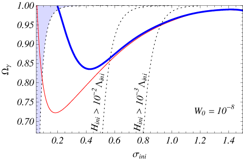
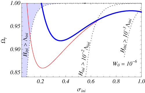
The space of initial conditions $\{\sigma_{\rm ini},\,\Omega_{\gamma}\}$ for which the system evolves to the overall minimum is plotted in Fig. 3; for all other initial conditions, $u$ and/or $\sigma$ overshoot. The thin/red curve gives the stabilization region for the KKLT potential with $u$ integrated out. The results agree with previous findings [12]: provided that the initial energy density is dominated by radiation, there is a large range of initial $\sigma_{\rm ini}$ leading to stabilization. Starting with initial values $\sigma_{\rm ini}$ to the left of the curve, the modulus picks up too much momentum and overshoots; starting with initial values $\sigma_{\rm ini}$ to the right of the curve, the modulus is too close to the minimum and there is not enough time to damp the field, with overshoot as result. Finally, we note that there is another small stabilization region for $\sigma_{\rm ini}$ close to the minimum $\sigma_{\rm min}$ (that is not displayed in the plot), for which the initial potential energy is less than the height of the barrier $V_{\rm ini}<V_{\rm max}$.

The equivalent curve for the full system is the thick/blue line. As expected, there are large discrepancies for small $\sigma_{\rm ini}$, and thus large $u_{\rm min}(\sigma_{\rm ini})$, whereas for larger $\sigma_{\rm ini}$ both systems give the same results. In terms of $n=(H/\Lambda)_{\rm ini}$, the deviations are negligible when this ratio drops below $n=10^{-2}$, and become large around $n=10^{-1}$ — Fig. 3 shows the lines for $n=1,\,10^{-2},\,10^{-3}$. This is almost independent of $W_{0}$, i.e. of the vacuum gravitino mass; the reason is that for such initial conditions the cubic term in the potential (3.1) is negligible, and all $W_{0}$ dependence drops out. This allows to restate the results in terms of $V_{\rm ini}$ as well: for $V_{\rm ini}\lesssim 10^{-7}$ the KKLT and full potential behave very similarly, whereas for $V_{\rm ini}\gtrsim 10^{-5}$ they deviate significantly.

We note that the smaller $W_{0}$ is, the longer it takes for the fields to roll down to their minima, and the longer they are exposed to damping; this explains why less initial radiation $\Omega_{\gamma}$ is needed for stabilization. Hence, for a TeV gravitino mass, $W_{0}\sim 10^{-14}$ and $c=1/10$, it is natural to expect the same behavior as in Fig. 3, with an even larger accessible range of $\Omega_{\gamma}$. In that case, one can further show that stabilization occurs at the unification-compatible point $g^{2}=1/2$.

As already stressed, the main reason for the breakdown of the KKLT approximation at large initial energy densities is due to the way the condensate is integrated out. Formally, the field $u$ should be integrated out at the level of the scalar potential. In the KKLT approach, however, this is not the case: the field $u$ is sent to zero in the Kähler potential, and replaced by its vev in the superpotential. The difference between the two approaches is easy to understand by studying the structure of the scalar potential (2.2); it gives rise to extra terms when the first approach is followed. The way heavy fields can be integrated out consistently in supergravity has been the center of renewed attention in the past months [30, 31, 32]. In this paper, we are dealing with intermediate energy ranges for which the extra terms in the scalar potential are not negligible. They have an impact on the dynamics of the system. Therefore, for small $\sigma_{\rm ini}$, the solution for $u_{\rm min}$ (2.4) is no longer a good approximation, and thus higher order terms in $u$ (the $u^{6}$-term in eq. (3.1)) have to be taken into account. Numerically, we find that the exact and the analytical solutions start to deviate more and more as we increase $V_{\rm ini}$. Notice that for $\sigma_{\rm ini}<0.2$ (or $V_{\rm ini}\gtrsim 10^{-3}$), the nontrivial minimum of $V_{F}(\sigma=\sigma_{\rm ini},\,u)$ along the $u$ direction disappears altogether, implying that gaugino condensation cannot occur. This explains the cutoff in the stabilization region in both plots. For $\sigma_{\rm ini}<0.2$, any $u_{\rm ini}$ leads to overshoot.

We now determine the stabilization region in $\{\sigma_{\rm ini},u_{\rm ini}\}$ space, considering initial conditions with both the modulus and the condensate displaced from the instantaneous minimum. Once again the fields start their evolution at rest.

The results for $W_{0}=10^{-6}$ and $\Omega_{\gamma}=0.95$ are shown in Fig. 4. The initial conditions $\{\sigma_{\rm ini},\,\delta u\equiv u_{\rm ini}-u_{\rm min}(\sigma_{\rm ini})\}$ leading to stabilization lie in the shaded/green area. A large range of modulus initial values leads to stabilization $0.2\lesssim\sigma_{\rm ini}\lesssim 0.6$, whereas only a small displacement in $\delta u$ is allowed. The reason for this is simple: the potential is much steeper in the condensate direction, even a comparatively small displacement $|\delta u|\lesssim 2\times 10^{-2}$ implies a large increase in $V_{\rm ini}$, and consequently leads to overshoot.

To address the likelihood of initial conditions leading to stabilization, it is therefore useful to consider not the initial field displacement, but rather the corresponding change in energy $V_{\rm ini}$. Given an initial energy $V_{\rm ini}$, and random initial conditions for both the modulus and condensate (but such that $V_{\rm ini}$ remains fixed), how large is the stabilization region in the space of initial conditions? In Fig. 4 are plotted the equipotential lines corresponding to $V_{\rm ini}=10^{-1},10^{-2},\dots,10^{-8}$. The lines are approximately orthogonal to $\delta u~=~0$ for small $\sigma_{\rm ini}$. Considering all initial conditions along one such line to be equally likely, the stabilization region is very small. Most initial conditions lead to overshoot. This is quite a different result than the conclusion one (naively) draws from the one-dimensional system with the condensate integrated out. Confining to initial conditions to the left of the maximum, a good proportion of initial conditions leads to stabilization.

The solid/orange line at $\delta u=0$ in Fig. 4 corresponds to a similar study in the effective KKLT model, without the dynamics of $u$. The points along that line at the left of the shaded/green area are initial conditions that appear to lead to stabilization from the one-dimensional standpoint. Once the dynamics of the condensate are considered, it is clear that those points are inconsistent.

As before, we consider the KKLT model with the condensate field $u$ integrated in and the parameters $c=1/7$ and $W_{0}=10^{-6}$. In addition, we take the initial radiation abundance to be $\Omega_{\gamma}=0.99$ and consider two different configurations with $r=-3/4\pi^{2}$ and $r=-0.04$ to illustrate the dependence on thermal corrections. The first case corresponds to an $\mathrm{SU}(2)$ pure Yang-Mills thermal sector and is thus the minimal $\left|r\right|$ achievable when the contribution (4.2) is the only component in radiation. Fig. 5 shows the set of admissible initial conditions $\{\sigma_{\rm ini},\,\delta u\}$ that lead to stabilization. The region surrounded by the dashed line corresponds to the result obtained in the previous section for zero temperature (cf. Fig. 4). Inside this region, we find those admissible initial conditions for $r=-0.04$ (light shaded) and $r=-3/4\pi^{2}\approx-0.076$ (dark shaded).

A few comments are in order. The region of stabilization clearly reduces when $\left|r\right|$ increases. For the SM gauge group $\mathrm{SU}(3)$$\times$$\mathrm{SU}(2)$, one finds $r\sim-0.1$, which leads to a considerable reduction of the allowed region. This implies that only for an even more fine-tuned value $\Omega_{\gamma}\sim 1$ does stabilization occur in a more realistic scenario. Also, the smallest value that the modulus can initially take depends on the thermal background. This happens because the higher the potential energy of the modulus $V_{\rm ini}$ is, the faster it rolls down to the position of the minimum. If the temperature is not sufficiently low, the modulus finds no minimum and consequently runs away. Similarly, if $\sigma$ starts too close to the local maximum of the modulus potential, at higher temperatures the modulus does not feel the attraction of the minimum and escapes.

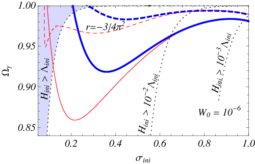
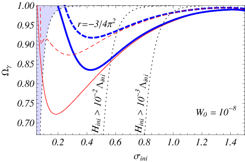
We explore also how the stabilization of the modulus depends on the initial radiation abundance $\Omega_{\gamma}$. In Fig. 6, we present our results including the condensate dynamics (blue/thick curves). In the left (right) panel we have set $W_{0}=10^{-6}$ ($10^{-8}$). The area over the solid (blue/thick) curve is the set of stabilization-compatible initial conditions at zero temperature. The area over the dashed (blue/thick) curve describes stabilization when thermal effects are included, with $r=-3/4\pi^{2}$. As expected, for low initial radiation abundance, the modulus runs away before the temperature decreases below $T_{\rm crit}$ and, therefore, stabilization is not possible. This sets a bound on the initial value of $\Omega_{\gamma}$, which in our examples is $\Omega_{\gamma,{\rm min}}\approx 0.98$ ($0.92$) for $W_{0}=10^{-6}$ ($10^{-8}$) with $r=-3/4\pi^{2}$.

We contrast these findings with those results obtained in the traditional way, i.e. in absence of the dynamical condensate field $u$ (red/thin curves). Note that the thin and the thick curves only coincide in a narrow region close to the stabilization point of $\sigma$ ($\sigma_{\rm min}\approx 1.22$ for $W_{0}=10^{-6}$ and $\sigma_{\rm min}\approx 1.68$ for $W_{0}=10^{-8}$). This implies that, integrating out the condensate is only valid for these points, that is, for initial conditions such that the Hubble rate $H_{\rm ini}$ is between two and three orders of magnitude lower than the condensation scale $\Lambda_{\rm ini}$ at the beginning of modulus evolution This observation is rather model independent and has to be taken into account in general when dealing with moduli stabilization driven by gaugino condensate in an evolving universe.

References

- [1] S. B. Giddings, S. Kachru, and J. Polchinski, Phys. Rev. D66 (2002), 106006, [hep-th/0105097].
- [2] M. Dine, R. Rohm, N. Seiberg, and E. Witten, Phys. Lett. B156 (1985), 55.
- [3] T. Banks and M. Dine, Phys. Rev. D50 (1994), 7454–7466, [hep-th/9406132].
- [4] T. Barreiro, B. de Carlos, and E. J. Copeland, Phys. Rev. D57 (1998), 7354–7360, [hep-ph/9712443].
- [5] G. Veneziano and S. Yankielowicz, Phys. Lett. B113 (1982), 231.
- [6] T. R. Taylor, G. Veneziano, and S. Yankielowicz, Nucl. Phys. B218 (1983), 493.
- [7] N. V. Krasnikov, Phys. Lett. B193 (1987), 37–40.
- [8] J. A. Casas, Phys. Lett. B384 (1996), 103–110, [hep-th/9605180].
- [9] S. Kachru, R. Kallosh, A. Linde, and S. P. Trivedi, Phys. Rev. D68 (2003), 046005, [hep-th/0301240].
- [10] T. Barreiro, B. de Carlos, and E. J. Copeland, Phys. Rev. D58 (1998), 083513, [hep-th/9805005].
- [11] R. Brustein, S. P. de Alwis, and P. Martens, Phys. Rev. D70 (2004), 126012, [hep-th/0408160].
- [12] T. Barreiro, B. de Carlos, E. Copeland, and N. J. Nunes, Phys. Rev. D72 (2005), 106004, [hep-ph/0506045].
- [13] C. van de Bruck, K.-Y. Choi, and L. M. H. Hall, JCAP 0711 (2007), 018, [0709.2810].
- [14] T. Barreiro, B. de Carlos, E. J. Copeland, and N. J. Nunes, Phys. Rev. D78 (2008), 063502, [0712.2394].
- [15] O. Lebedev, C. Papineau, and M. Postma, (2009), 0907.4630.
- [16] R. Kappl et al., Phys. Rev. Lett. 102 (2009), 121602, [0812.2120].
- [17] C. P. Burgess, J. P. Derendinger, F. Quevedo, and M. Quiros, Annals Phys. 250 (1996), 193–233, [hep-th/9505171].
- [18] F. Cachazo, M. R. Douglas, N. Seiberg, and E. Witten, JHEP 12 (2002), 071, [hep-th/0211170].
- [19] E. Witten, Nucl. Phys. B202 (1982), 253.
- [20] M. A. Shifman and A. I. Vainshtein, (1999), hep-th/9902018.
- [21] K. Becker, M. Becker, M. Haack, and J. Louis, JHEP 06 (2002), 060, [hep-th/0204254].
- [22] M. Berg, M. Haack, and B. Kors, JHEP 11 (2005), 030, [hep-th/0508043].
- [23] O. DeWolfe and S. B. Giddings, Phys. Rev. D67 (2003), 066008, [hep-th/0208123].
- [24] H.-Y. Chen, Y. Nakayama, and G. Shiu, (2009), 0905.4463.
- [25] S. B. Giddings and A. Maharana, Phys. Rev. D73 (2006), 126003, [hep-th/0507158].
- [26] R. Brustein and P. J. Steinhardt, Phys. Lett. B302 (1993), 196–201, [hep-th/9212049].
- [27] D. H. Lyth and T. Moroi, JHEP 05 (2004), 004, [hep-ph/0402174].
- [28] C. Papineau, M. Postma, and S. Ramos-Sánchez, work in progress.
- [29] L. Kofman et al., JHEP 05 (2004), 030, [hep-th/0403001].
- [30] A. Achucarro, S. Hardeman, and K. Sousa, Phys. Rev. D78 (2008), 101901, [0806.4364].
- [31] D. Gallego and M. Serone, JHEP 01 (2009), 056, [0812.0369].
- [32] L. Brizi, M. Gómez-Reino, and C. A. Scrucca, Nucl. Phys. B820 (2009), 193–212, [0904.0370].
- [33] M. T. Grisaru and P. C. West, Nucl. Phys. B254 (1985), 249.
- [34] W. Buchmüller, K. Hamaguchi, and M. Ratz, Phys. Lett. B574 (2003), 156–161, [hep-ph/0307181].
- [35] K. Kajantie, M. Laine, K. Rummukainen, and Y. Schroder, Phys. Rev. D67 (2003), 105008, [hep-ph/0211321].
- [36] W. Buchmüller, K. Hamaguchi, O. Lebedev, and M. Ratz, Nucl. Phys. B699 (2004), 292–308, [hep-th/0404168].
- [37] W. Buchmüller, K. Hamaguchi, O. Lebedev, and M. Ratz, JCAP 0501 (2005), 004, [hep-th/0411109].