Classification by Set Cover: The Prototype Vector Machine

Consider the two sets $\mathcal{X}$ and $\mathcal{Z}$ but without the labels $\mathbf{y}$. Let $D$ be the $n\times m$ matrix of dissimilarities, with $D_{ij}=d(\mathbf{x}_{i},\mathbf{z}_{j})$ for each $\mathbf{x}_{i}\in\mathcal{X}$ and $\mathbf{z}_{j}\in\mathcal{Z}$ (note: $d$ need not be a metric), and fix $\epsilon>0$. The goal is to find the smallest subset of points $\mathcal{P}\subseteq\mathcal{Z}$ such that every point $\mathbf{x}_{i}\in\mathcal{X}$ is within $\epsilon$ of some point in $\mathcal{P}$ (i.e., there exists $\mathbf{z}_{j}\in\mathcal{P}$ with $d(\mathbf{x}_{i},\mathbf{z}_{j})<\epsilon$). Let $B_{\epsilon}(\mathbf{x})=\{\mathbf{x}^{\prime}\in\mathbf{R}^{p}:d(\mathbf{x}^{\prime},\mathbf{x})<\epsilon\}$ denote the ball of radius $\epsilon$ centered at $\mathbf{x}$. Introducing the indicator variables

this problem can be stated as an integer program:

The objective is simply $|\mathcal{P}|$. The summation in the constraint counts the number of elements of $\mathcal{P}$ that are within $\epsilon$ of the point $\mathbf{x}_{i}$, so a feasible solution to the above integer program is one that has at least one prototype within $\epsilon$ of each training point.

From a machine learning point of view, set cover can be seen as a clustering problem in which we wish to find the smallest number of clusters such that every point is within $\epsilon$ of at least one cluster center. In the language of vector quantization, it seeks the smallest codebook (restricted to $\mathcal{Z}$) such that no vector is distorted by more than $\epsilon$ [Tipping and Schölkpf, 2001].

We now express the three properties above as an integer program, taking as a starting point the set cover problem of Equation 2. Property (b) suggests that in certain cases it may be necessary to leave some points of class $l$ uncovered. For this reason, we adopt a prize-collecting set cover framework for our problem (i.e., we assign a cost to each covering set, a penalty for being uncovered to each point, and then find the minimum-cost partial cover, Könemann et al. 2006). Let $\alpha_{j}^{(l)}\in\{0,1\}$ indicate whether we choose $\mathbf{z}_{j}$ to be in $\mathcal{P}_{l}$ (i.e., to be a prototype for class $l$). We define the PVM to be a solution to the following integer program:

We have introduced two slack variables, $\xi_{i}$ and $\eta_{i}$, per training point $\mathbf{x}_{i}$. Constraint (3a) enforces that each training point be covered by at least one ball of its own class-type (otherwise $\xi_{i}=1$). Constraint (3b) expresses the condition that training point $\mathbf{x}_{i}$ not be covered with balls of other classes (otherwise $\eta_{i}>0$). In particular, the slack variables can be interpreted as

• •

  $\xi_{i}=\begin{cases}1&\text{if~}\mathbf{x}_{i}\text{~is not covered by a class-$y_{i}$ prototype ball}\\ 0&\text{otherwise~}\end{cases}$

• •

  $\eta_{i}=$ Number of prototypes covering $\mathbf{x}_{i}$ that are not of class $y_{i}$.

Finally, $\lambda\geq 0$ is a parameter specifying the cost of adding a prototype. Its effect is to control the number of prototypes chosen (corresponding to property (c) of the last section). We generally choose $\lambda=1/n$, so that property (c) serves only as a “tie-breaker” for choosing among multiple solutions that do equally well on properties (a) and (b). Hence, in words, we are minimizing the sum of (a) the number of points left uncovered, (b) the number of points wrongly covered, and (c) the number of covering balls (multiplied by $\lambda$). The resulting method has a single tuning parameter, $\epsilon$ (the ball radius), which can be estimated by cross validation.

We show in the Appendix that the PVM integer program is equivalent to $L$ separate prize-collecting set cover problems. Let $\mathcal{X}_{l}=\{\mathbf{x}_{i}\in\mathcal{X}:y_{i}=l\}$. Then, for each class $l$, the set $\mathcal{P}_{l}\subseteq\mathcal{Z}$ is given by the solution to

where $C_{l}(j)$ is the cost of adding $\mathbf{z}_{j}$ to $\mathcal{P}_{l}$ and a unit penalty is charged for each point $\mathbf{x}_{i}$ of class $l$ left uncovered. The cost of a covering set for the PVM is the number of miscovered points plus a baseline charge of $\lambda$:

A well-known approach for the set cover problem is to relax the integer constraint $\alpha_{j}^{(l)}\in\{0,1\}$ by replacing it with $0\leq\alpha_{j}^{(l)}\leq 1$. The result is a linear program (LP), which is convex and easily solved with any LP solver. The result is subsequently rounded to recover a feasible (though not necessarily optimal) solution to the original integer program.

Let $\{\alpha_{j}^{*(l)}\}$ denote a solution to the LP. Since our solution in general will be fractional, we adopt the following rounding strategy to produce an integral solution: For each $j\in\{1,\ldots,m\}$ and $l\in\{1,\ldots,L\}$, we independently draw $A_{j}^{(l)}\sim\text{Bernoulli}(\alpha_{j}^{*(l)})$. Notice that $\alpha_{j}^{*(l)}\in[0,1]$, so this approach is well-defined. Let $S_{i}$ and $T_{i}$ denote the slack (corresponding to $\xi_{i}$ and $\eta_{i}$) incurred by the rounded solution $\{A_{j}^{(l)}\}$. These random variables are given by

The randomized rounding algorithm is as follows (with $B$ typically in the hundreds):

For $b=1,\ldots,B$: 1. Draw independently $A_{j}^{(l)}(b)\sim\text{Bernoulli}(\alpha_{j}^{*(l)})$. 2. Find the corresponding $S_{i}(b)$, $T_{i}(b)$ making this a feasible solution. (using Equation 4) 3. Evaluate objective $OBJ(b)=\sum_{i=1}^{n}(S_{i}(b)+T_{i}(b))+\lambda\sum_{j,l}A_{j}^{(l)}(b)$. Return $\{A_{j}^{(l)}(b)\}$ with minimum $OBJ(b)$.

In the Appendix, we prove that the expected objective on any iteration satisfies

where $OPT_{LP}=\sum_{i=1}^{n}{(\xi^{*}_{i}+\eta^{*}_{i})}+\lambda\sum_{j=1}^{n}{\sum_{l=1}^{L}{\alpha_{j}^{*(l)}}}$ is the optimal value of the LP (which is a lower bound on the integer program’s optimal value).

One disadvantage of this approach is that it requires solving an LP, which can be relatively slow and memory-intensive for large data sets. The approach we describe next is much lighter-weight and is thus our preferred method.

Another well-known approximation algorithm for the set cover problem is the greedy algorithm [Vazirani, 2001]. At each step, we add the prototype that has the least ratio of cost to number of points newly covered. However, here we present a less standard greedy algorithm which has certain practical advantages over the standard greedy approach and does not in our experience do noticeably worse in minimizing the PVM objective. At each step we find the $\mathbf{z}_{j}\in\mathcal{Z}$ and class $l$ for which adding $\mathbf{z}_{j}$ to $\mathcal{P}_{l}$ most decreases the objective function. That is, we find the $(\mathbf{z}_{j},l)$ pair with the best tradeoff of covering previously uncovered training points of class $l$ while avoiding covering points of other classes. The incremental improvement of going from $(\mathcal{P}_{1},\ldots,\mathcal{P}_{L})$ to $(\mathcal{P}_{1},\ldots,\mathcal{P}_{l-1},\mathcal{P}_{l}\cup\{\mathbf{z}_{j}\},\mathcal{P}_{l+1},\ldots,\mathcal{P}_{L})$ can be denoted by $\Delta\text{Obj}(\mathbf{z}_{j},l)=\Delta\xi(\mathbf{z}_{j},l)-\Delta\eta(\mathbf{z}_{j},l)-\lambda$ where

The greedy algorithm is simply as follows:

1. Start with $\mathcal{P}_{l}=\emptyset$ for each class $l$. 2. While $\Delta\text{Obj}(\mathbf{z}^{*},l^{*})>0$: • Find $(\mathbf{z}^{*},l^{*})=\operatornamewithlimits{argmax}_{(\mathbf{z}_{j},l)}{\Delta\text{Obj}(\mathbf{z}_{j},l)}$. • Let $\mathcal{P}_{l^{*}}:=\mathcal{P}_{l^{*}}\cup\{\mathbf{z}^{*}\}$.

The PVM depends on all of the $\mathbf{x}_{i}$ and $\mathbf{z}_{j}$ only through the pairwise dissimilarities $d(\mathbf{x}_{i},\mathbf{z}_{j})$ and can accept any matrix with non-negative entries. This allows it to share in the benefits of kernel methods by using a kernel-based distance.²² 2 Given a kernel $K(x,x^{\prime})$, we can use the distance $$d(x,x^{\prime})=\sqrt{K(x,x)+K(x^{\prime},x^{\prime})-2K(x,x^{\prime})}$$ Also, for problems in the $p\gg n$ realm, using distances that effectively lower the dimension can lead to improvements. For instance, we have achieved gains in classification accuracy in some $p\gg n$ simulations by using the DANN-distance [Hastie and Tibshirani, 1996], which is a supervised measure of distance. Additionally, in certain problems (e.g., in proteomics, see Section 6.3) the data may not be readily embedded in a vector space. In such a case, we may still apply the PVM if pairwise dissimilarities are available.

Finally, given any dissimilarity $d$, we may instead use $\tilde{d}$, defined by $\tilde{d}(\mathbf{x},\mathbf{z})=|\{\mathbf{x}_{i}\in\mathcal{X}:d(\mathbf{x}_{i},\mathbf{z})\leq d(\mathbf{x},\mathbf{z})\}|$. Using $\tilde{d}$ induces $\epsilon$-balls $B_{\epsilon}(\mathbf{z}_{j})$ containing the $(\lfloor\epsilon\rfloor-1)$ nearest training points to $\mathbf{z}_{j}$.

Another inherent flexibility of the PVM is in the choice of $\mathcal{Z}$, the set of potential prototypes. While $\mathcal{Z}=\mathcal{X}$ is a standard choice, we have experimented with other possibilities as well. For example, if we are also given a set of unlabeled data (e.g., a test set), we may add these examples as potential prototypes, yielding a semi-supervised version of the PVM. Doing so preserves the property that all prototypes are actual examples (rather than arbitrary points in $\mathbf{R}^{p}$).

We believe that having prototypes confined to lie on actual observed points is desirable for interpretability. However, in circumstances in which this property is not needed, $\mathcal{Z}$ may be further augmented to include other points. For example, one could run $K$-means on each class’s points individually (or on the training set as a whole) and add these $L\cdot K$ centroids to $\mathcal{Z}$. This method seems to help especially in high dimensional problems where constraining all prototypes to lie on data points suffers from the curse of dimensionality. Another successful choice for $\mathcal{Z}$ is to sample uniformly within the convex hull of each class’s training points.

For demonstration purposes, we consider a three-class example with $p=2$. Each class was generated as a mixture of 10 Gaussians (details given in the Appendix). Figure 1 shows the PVM solution for a range of values of the tuning parameter $\epsilon$. In Figure 2, we display the classification boundaries for the PVM, $K$-medoids, and LVQ (taking the lowest test error solution for each method). Since we generated this example from a known model, we are able to compute the Bayes boundary. We see that the PVM succeeds in capturing the shape of the boundary. The erratic boundary of $K$-medoids highlights an advantage of the PVM over $K$-medoids; the latter does not consider the relation between classes when choosing prototypes and therefore does not perform well when classes overlap.

We apply the PVM to the USPS handwritten digits data set which consists of a training set of $n=7291$ grayscale ($16\times 16$ pixel) images of handwritten digits 0-9 (and $2007$ test images). We run the PVM for a range of values of $\epsilon$ from the minimum interpoint distance (in which the PVM retains the entire training set and so reduces to 1-NN classification) to approximately the $14^{\text{th}}$ percentile of interpoint distances.

The lefthand panel of Figure 3 shows the test error as a function of the number of prototypes for several methods using the Euclidean metric. Since both LVQ and $K$-means can place prototypes anywhere in the feature space, which is advantageous in high-dimensional problems, we also allow PVM to select prototypes that do not lie on the training points by augmenting $\mathcal{Z}$. In this case, we run 10-means clustering on each class separately and then add these resulting 100 points to $\mathcal{Z}$ (in addition to $\mathcal{X}$).

The notion of the tangent distance between two such images was introduced by Simard et al. [1993] to account for certain invariances in this problem (e.g., the thickness and orientation of a digit are not relevant factors when we consider how similar two digits are). Use of tangent distance with 1-NN attained the lowest test errors of any method [Hastie and Simard, 1998]. Since the PVM operates on an arbitrary dissimilarities matrix, we can easily use the tangent distance in place of the standard Euclidean metric. The righthand panel of Figure 3 shows the test errors when tangent distance is used. $K$-medoids similarly readily accommodates any dissimilarity. While LVQ has been generalized to arbitrary differentiable metrics, there does not appear to be generic, off-the-shelf software available. The lowest test error attained by the PVM is 2.49% with a 3372-prototype solution (compared to 1-NN’s 3.09%).³³ 3 Hastie and Simard [1998] report a 2.6% test error for 1-NN on this data set. The difference may be due to implementation details of the tangent distance. Also, we can see that for a wide range of $\epsilon$ values we get a solution with test error comparable to that of 1-NN, but requiring far fewer prototypes. An advantageous feature of the PVM is that it automatically chooses the number of prototypes per class to use. In this example, it is interesting to see the class-frequencies of prototypes (see Table 1).

The most dramatic feature of this solution is that it only retains seven of the 1005 examples of the digit 1. This reflects the fact that, relative to other digits, the digit 1 has the least variation when handwritten. Indeed, the average (tangent) distance between digit 1’s in the training set is less than half that of any other digit (the second least variable digit is 7).

In this example, we took $\mathcal{Z}=\mathcal{X}$, so that each prototype is an actual handwritten digit from the training set (rather than being some linear combination of many handwritten digits). Figures 4 and 5 show images of the first 88 prototypes (of 3372) selected by the greedy algorithm. Above each image of Figure 4 is the number of training images previously uncovered that were correctly covered by the addition of this prototype and, in parentheses, the number of training points that are miscovered by this prototype. For example, we can see that the first prototype selected by the greedy algorithm, which was a “1,” covered 986 training images of 1’s and four training images that were not of 1’s. These four training images are shown in Figure 6. Indeed, all of them look very much like 1’s, which explains the algorithm’s confusion.

The lefthand panel of Figure 7 shows the improvement in the PVM objective, $\Delta\xi-\Delta\eta$, after each step of the greedy algorithm, revealing an interesting feature of the solution: we find that after the first 458 prototypes are added, each remaining prototype covers only one training point. Since in this example we took $\mathcal{Z}=\mathcal{X}$ (and since a point always covers itself), this means that the final 2914 prototypes were chosen to cover only themselves. In this sense, we see that the PVM provides a sort of compromise between a sparse nearest prototype classifier and 1-NN. The compromise is determined by the prototype-cost parameter $\lambda$. If $\lambda>1$, the algorithm does not enter the 1-NN regime.

The righthand panel of Figure 7 shows the improvement in test error gained by running the greedy algorithm beyond the first 88 steps (corresponding to the $\lambda=6$ solution). It is interesting to look at elements of the test set that are misclassified when we use just the 88 prototypes but are correctly classified when using the complete PVM-greedy solution (with all 3372 prototypes). There are 276 (out of 2007) such elements. Figure 8 shows a randomly chosen seven examples of these test points.

In our next example, we present a case in which the patterns are not naturally represented as vectors in $\mathbf{R}^{p}$. Leslie et al. [2004] study the problem of classification of proteins based on their amino acid sequences. They introduce a measure of similarity between protein sequences called the mismatch kernel. The general idea is that two sequences should be considered similar if they have a large number of short sequences in common (where two short sequences are considered the same if they have no more than a specified number of mismatches). We take as input a $1708\times 1708$ matrix with $K_{ij}$ containing the value of the normalized mismatch kernel evaluated between proteins $i$ and $j$ (the data and software are from Leslie et al. 2004). The proteins fall into two classes, “Positive” and “Negative,” according to whether they belong to a certain protein family. We compute pairwise distances from this kernel via $D_{ij}=\sqrt{K_{ii}+K_{jj}-2K_{ij}}$ and then run the PVM and $K$-medoids. Figure 9 shows the 10-fold cross-validated errors for the PVM and $K$-medoids. For the PVM, we take a range of equally-spaced quantiles of the pairwise distances from the minimum to the median for the parameter $\epsilon$. For $K$-medoids, we take as parameter the fraction of proteins in each class that should be prototypes. This choice of parameter allows the classes to have different numbers of prototypes, which is important in this example because the classes are greatly imbalanced (only 45 of the 1708 proteins are in class “Positive”). The minimum CV-error (1.76%) is attained by PVM using about 870 prototypes (averaged over the 10 models fit for that value of $\epsilon$). This error is identical to the minimum CV-error of a support vector machine (tuning the cost parameter) trained using this kernel.

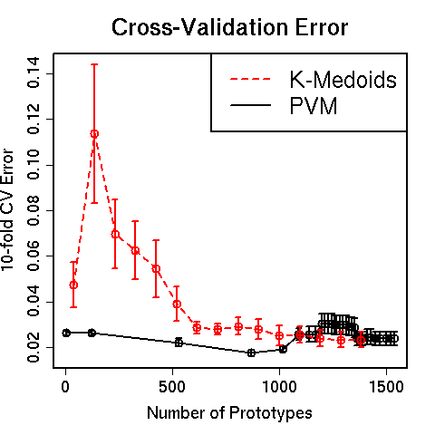
Fitting a model to the whole data set with the selected value of $\epsilon$, the PVM chooses 26 prototypes (of 45) for class “Positive” and 907 (of 1663) for class “Negative.”

Finally, we run the PVM on six data sets from the UCI Machine Learning Repository [Asuncion and Newman, 2007] and compare its performance to that of 1-NN (i.e., retaining all training points as prototypes), $K$-medoids, and LVQ. We randomly select 2/3 of each data set for training and use the remainder as a test set. Ten-fold cross-validation (and the “1 standard error rule,” Hastie et al. 2009) is performed on the training data to select a value for each method’s tuning parameter (except for 1-NN). Table 2 reports the error on the test set and the number of prototypes selected for each method. We see that in most cases PVM is able to do as well as or better than 1-NN but with a significant reduction in prototypes. No single method does best on all of the data sets.

References

- Asuncion and Newman [2007] A. Asuncion and D.J. Newman. UCI machine learning repository, 2007. URL http://www.ics.uci.edu/mlearn/MLRepository.html.
- Devijver and Kittler [1982] P.A. Devijver and J.V. Kittler. Pattern Recognition: a Statistical Approach. Prentice-Hall, Englewood Cliffs, N.J., 1982.
- Feige [1998] U. Feige. A threshold of ln n for approximating set cover. Journal of the ACM, 45(4):634–652, 1998. ISSN 0004-5411.
- Hart [1968] P. Hart. The condensed nearest-neighbor rule. IEEE Trans. Inform. Theory, 14:515–516, 1968.
- Hastie and Simard [1998] T. Hastie and P. Y. Simard. Models and metrics for handwritten digit recognition. Statistical Science, 13:54–65, 1998.
- Hastie and Tibshirani [1996] T. Hastie and R. Tibshirani. Discriminant adaptive nearest-neighbor classification. IEEE Pattern Recognition and Machine Intelligence, 18:607–616, 1996.
- Hastie et al. [2009] T. Hastie, R. Tibshirani, and J. Friedman. The Elements of Statistical Learning; Data Mining, Inference and Prediction, Second Edition. Springer Verlag, New York, 2009.
- Kohonen [2001] T. Kohonen. Self-Organizing Maps. Springer-Verlag, 2001.
- Könemann et al. [2006] J. Könemann, O. Parekh, and D. Segev. A unified approach to approximating partial covering problems. In ESA’06: Proceedings of the 14th conference on Annual European Symposium, pages 468–479, London, UK, 2006. Springer-Verlag.
- Leslie et al. [2004] C. S. Leslie, E. Eskin, A. Cohen, J. Weston, and W. S. Noble. Mismatch string kernels for discriminative protein classification. Bioinformatics, 20(4):467–476, 2004.
- Ripley [2005] B. D. Ripley. Pattern Recognition and Neural Networks. Cambridge University Press, 2005.
- Simard et al. [1993] P. Y. Simard, Y. A. Le Cun, and J. S. Denker. Efficient pattern recognition using a new transformation distance. In Advances in Neural Information Processing Systems, pages 50–58, San Mateo, CA, 1993. Morgan Kaufman.
- Tipping and Schölkpf [2001] M.E. Tipping and B. Schölkpf. A kernel approach for vector quantization with guaranteed distortion bounds. Artificial Intelligence and Statistics, pages 129–134, 2001.
- Vazirani [2001] V. Vazirani. Approximation Algorithms. Springer-Verlag, 2001.
- Weinberger and Saul [2009] K. Q. Weinberger and L. K. Saul. Distance metric learning for large margin nearest neighbor classification. Journal of Machine Learning Research, 10:207–244, 2009.
Appendix A PVM’s relation to prize-collecting set cover
Claim: Solving the PVM integer program is equivalent to solving prize-collecting set cover problems.
Proof.
Recall that the PVM integer program is given by