跳到论文正文
W Papers独立论文阅读器 arXiv:0908.2172 论文正文 计算阅读时间 · 0%
引用这篇论文根据当前论文元数据生成,正式投稿前建议核对。


License: arXiv.org perpetual non-exclusive license
arXiv:0908.2172v2 [cond-mat.quant-gas] 22 Sep 2009

Vortex structures in rotating Bose-Einstein condensates

S. I. Matveenko1,2, D. Kovrizhin3, S. Ouvry2, and G. V. Shlyapnikov2,4 Affiliation: 1L.D. Landau Institute for Theoretical Physics, Kosygina Str. 2, 119334, Moscow, Russia
2 Laboratoire de Physique Théorique et Modéles Statistiques, Université Paris Sud, CNRS,
91405 Orsay, France
3Theoretical Physics, Oxford University, 1 Keble road, OX1 3NP, Oxford, UK
4Van der Waals-Zeeman Institute, University of Amsterdam, Valckenierstraat 65/67,
1018 XE Amsterdam, The Netherlands
August 24, 2026
Abstract

We present an analytical solution for the vortex lattice in a rapidly rotating trapped Bose-Einstein condensate (BEC) in the lowest Landau level and discuss deviations from the Thomas-Fermi density profile. This solution is exact in the limit of a large number of vortices and is obtained for the cases of circularly symmetric and narrow channel geometries. The latter is realized when the trapping frequencies in the plane perpendicular to the rotation axis are different from each other and the rotation frequency is equal to the smallest of them. This leads to the cancelation of the trapping potential in the direction of the weaker confinement and makes the system infinitely elongated in this direction. For this case we calculate the phase diagram as a function of the interaction strength and rotation frequency and identify the order of quantum phase transitions between the states with a different number of vortex rows.

pacs
03.75.Lm, 05.30.Jp, 73.43.Nq

I Introduction

Rapidly rotating Bose-condensed gases constitute a novel class of many-body systems where the ground state properties are governed by a collective behavior of nucleated vortices [1, 2]. A harmonically trapped dilute Bose-Einstein condensate (BEC) strongly confined in the zz direction, is essentially two-dimensional in the (x,y)(x,y) plane. When the rotation frequency along the zz axis becomes close to the trapping frequencies in the xx and yy directions, the BEC gas can be described as a system of interacting bosons in the lowest Landau level. The single-particle Hamiltonian is similar to that of a charged particle in a strong magnetic field, and the regime of fast rotation of neutral bosons presents an analogy with Quantum Hall Effect. Due to the presence of remaining harmonic trapping, the lowest Landau level (LLL) is not degenerate. However, analytic properties of the LLL wave functions generate an effective long-range interaction between the bosons, which results in an interesting physics.

If the rotation frequency is not very close to the trap frequency, then the number of vortices is much smaller than the number of particles. Under these conditions the system is in the so-called mean-field Quantum Hall regime and can be described by a macroscopic wavefunction Ψ⁡(𝐫)\Psi(\bf r) in the lowest Landau level. In this limit the vortices generically arrange themselves in a lattice. An increase in the rotation frequency increases the number of vortices and eventually it becomes comparable with the number of particles. This leads to melting of the vortex lattice and to the appearance of strongly correlated states [1, 2]. The “mean-field Quantum Hall regime” for trapped bosons has been introduced by Ho [3] and studied in a number of papers where the vortex lattice structures have been obtained numerically in the case of a circularly symmetric trapping potential [4, 5, 6, 7].

In this paper we consider a rotating BEC in the lowest Landau level in the mean-field regime and obtain an analytical solution for the vortex lattice of the harmonically trapped symmetric 2D gas. This solution is exact in the limit of a large number of vortices, and we discuss deviations from the Thomas-Fermi density profile. We then turn to the case of the “narrow channel” geometry, which is realized when the confining frequencies in the xx and yy directions are different, and the rotation frequency is equal to the smallest of them. Then, in the rotating frame, the gas becomes extremely elongated in the direction of the smaller frequency, as has been demonstrated in the ENS experiment with thermal bosons [8]. This is an extreme case of a rapidly rotating 2D gas in an asymmetric harmonic potential, discussed in relation to the density profile of the gas and the density of vortices in Ref. [9]. Some vortex structures of the asymmetric rapidly rotating BEC have been discussed and calculated in Refs. [10, 11, 12, 13]. In the narrow channel geometry, the excitation spectrum of a weakly interacting BEC without vortices exhibits a “roton-maxon” structure [14]. The phase transition to the state with a vortex row occurs when the roton energy reaches zero under an increase in the rotation frequency or in the strength of interaction between the bosons. A further increase of these quantities increases the number of vortex rows through a set of quantum phase transitions [14, 15]. We classify these transitions and find an analytical solution for the vortex lattice in the narrow channel, which is exact in the limit of a large number of vortex rows.

II Gross-Pitaevskii equation in the lowest Landau level. Solution for a symmetric harmonic potential

Consider a system of bosonic neutral atoms strongly confined in the zz direction by an external trapping potential with frequency ωz\omega_{z} such that the bosons are in the ground state of the ωz\omega_{z} harmonic well and become essentially two-dimensional in the (x,y)(x,y)-plane. The bosons are confined in this plane by a harmonic trapping potential V⁡(𝐫)V({\bf r}), with 𝐫={x,y}{\bf r}=\{x,y\}, and the trap is rotating around the zz axis with frequency Ω\Omega. In the mean-field Quantum Hall limit, we assume to zero order that all particles are in the same macroscopic quantum state described by the wavefunction ψ⁡(𝐫)\psi({\bf r}). In the rotating frame the Gross-Pitaevskii equation for ψ⁡(𝐫)\psi({\bf r}) reads:

𝐩^22​m​ψ+g​|ψ|2​ψ+V⁡(𝐫)​ψ−Ω​L^z​ψ=μ​ψ,\frac{\hat{{\bf p}}^{2}}{2m}\psi+g|\psi|^{2}\psi+V({\bf r})\psi-\Omega\hat{L}_{z}\psi=\mu\psi, (1)

where 𝐩^\hat{{\bf p}} is the momentum operator, mm is the particle mass, L^z\hat{L}_{z} is the operator of the orbital angular momentum, μ\mu is the chemical potential, and ψ\psi is normalized to the total number of particles NN. Equation (1) is obtained for a short-range interaction between particles, and the 2D coupling constant gg can be expressed through the 3D scattering length asa_{s}. If the harmonic oscillator length in the zz direction, lz=ℏ/m​ωzl_{z}=\sqrt{\hbar/m\omega_{z}}, is much larger than |as||a_{s}| and the characteristic radius of interparticle interaction, then we have [16]:

g=2​2​π​ℏ2​asm​lz.g=\frac{2\sqrt{2\pi}\hbar^{2}a_{s}}{ml_{z}}. (2)

We will study Eq. (1) projected onto the lowest Landau level. A general procedure of obtaining the projected equation is described in the Appendix, and here we outline the method.

The single-particle Hamiltonian for rotating neutral atoms is equivalent to the Hamiltonian of a charged particle in a uniform magnetic field BB along the zz axis. The field is such that half the cyclotron frequency ωc=B/2​m\omega_{c}=B/2m (in units of charge divided by the light velocity) is identified with the rotation frequency Ω\Omega, and the vector-potential in the symmetric gauge is 𝐀=[𝐁×𝐫]/2=m⁡[𝛀×𝐫]{\bf{A}}=[{\bf B}\times{\bf r}]/2=m[{\bf{\Omega}}\times{\bf r}]. In the case of a symmetric external harmonic potential V⁡(r)=m​ω2​r2/2V(r)=m\omega^{2}r^{2}/2 the single-particle Hamiltonian reads:

H=𝐩^22​m−Ω​L^z+12​m​ω2​r2=12​m​(𝐩^−e​𝐀/c)2+12​m​(ω2−Ω2)​r2,H=\frac{\hat{{\bf p}}^{2}}{2m}-\Omega\hat{L}_{z}+\frac{1}{2}m\omega^{2}r^{2}=\frac{1}{2m}{(\hat{{\bf p}}-e{\bf{A}}/c)^{2}}+\frac{1}{2}m(\omega^{2}-\Omega^{2})r^{2}, (3)

At the critical rotation frequency Ω=ω\Omega=\omega the residual confining potential vanishes, and the harmonic oscillator length l=(ℏ/m​ω)1/2l=(\hbar/m\omega)^{1/2} of the initial trapping potential V⁡(r)V(r) coincides with the ”magnetic length” (ℏ/m​Ω)1/2(\hbar/m\Omega)^{1/2}. One then has an ”infinite plane” geometry actively studied with respect to the ground state of interacting bosons [17, 18, 19, 20, 21].

Below the critical rotation frequency, Ω<ω\Omega<\omega and (ω−Ω)≪Ω(\omega-\Omega)\ll\Omega, the energy eigenstates are associated with the Landau levels of a charged particle in the uniform magnetic field, and the presence of the residual confining potential lifts the LLL degeneracy. A complete set of LLL eigenfunctions is given by

Ψn​(z,z¯)=znl​π​n!​exp⁡[−z​z¯2],\Psi_{n}(z,{\bar{z}})=\frac{z^{n}}{l\sqrt{\pi n!}}\exp\left[-\frac{z{\bar{z}}}{2}\right], (4)

with z,z¯=(x±i​y)/lz,{\bar{z}}=(x\pm iy)/l, and nn being a non-negative integer. An arbitrary function in the LLL can be written as a linear superposition of the LLL eigenstates and represented in the form:

Ψ⁡(z,z¯)=f⁡(z)l​exp⁡[−z​z¯2],\Psi(z,{\bar{z}})=\frac{f(z)}{l}\exp\left[-\frac{z{\bar{z}}}{2}\right], (5)

where f⁡(z)f(z) is an analytic function of zz. The projection operator onto the LLL is written as

P^=∑n|n⟩​⟨n|,\hat{P}=\sum_{n}|n\rangle\langle n|, (6)

where ⟨z|n⟩=Ψn​(z,z¯)\langle z|n\rangle=\Psi_{n}(z,{\bar{z}}) is given by Eq. (4). Acting with the operator P^\hat{P} on an arbitrary function ϕ(z,z¯)=[f(z,z¯)/l]exp(−zz¯/2)\phi(z,{\bar{z}})=[f(z,\bar{z})/l]\exp(-z{\bar{z}}/2) one obtains:

P^ϕ(z,z¯)=∑n=0∞∫Ψn(z,z¯)Ψn∗(z′,z¯′)ϕ(z′,z¯′)dz′dz¯′=[f~(z)/l]exp(−zz¯/2),\hat{P}\phi(z,{\bar{z}})=\sum_{n=0}^{\infty}\int\Psi_{n}(z,{\bar{z}})\Psi_{n}^{*}(z^{\prime},{\bar{z}}^{\prime})\phi(z^{\prime},{\bar{z}}^{\prime})dz^{\prime}d{\bar{z}}^{\prime}=[\tilde{f}(z)/l]\exp(-z{\bar{z}}/2), (7)

with d​z′​d​z′¯=d​x′​d​y′/l2dz^{\prime}d\bar{z^{\prime}}=dx^{\prime}\,dy^{\prime}/l^{2}, and an analytic function f~​(z)\tilde{f}(z) which is given by

f~​(z)=1π​∫d​z′​𝑑z′¯​f​(z′,z′¯)​exp⁡(z​z¯′−z′​z′¯).\tilde{f}(z)=\frac{1}{\pi}\int dz^{\prime}d\bar{z^{\prime}}f(z^{\prime},\bar{z^{\prime}})\exp(z\bar{z}^{\prime}-z^{\prime}\bar{z^{\prime}}). (8)

This formalism was introduced by Bargmann [22] and developed by Girvin and Jach [23] in relation to Quantum Hall physics.

In the case of interacting bosons one can still project the many-body Hamiltonian onto the lowest Landau level provided that the interactions are much smaller than the cyclotron gap, i.e. n2​D​g≪2​ℏ​Ωn_{2D}g\ll 2\hbar\Omega, where n2​Dn_{2D} is the two-dimensional particle density [1, 2]. Acting with the LLL projector P^\hat{P} onto the Gross-Pitaevskii equation (1) results in the projected equation (see Refs. [5, 12] and Appendix):

ℏ​(ω−Ω)​z​∂zf⁡(z)+N​gπ​l2​∫d​z′​𝑑z′¯​|f⁡(z′)|2​f​(z′)​exp⁡(z​z¯′−2​z′​z¯′)=μ~​f​(z),\hbar(\omega-\Omega)z\partial_{z}f(z)+\frac{Ng}{\pi l^{2}}\int dz^{\prime}d\bar{z^{\prime}}|f(z^{\prime})|^{2}f(z^{\prime})\exp(z\bar{z}^{\prime}-2z^{\prime}\bar{z}^{\prime})=\tilde{\mu}f(z), (9)

where μ~=μ−ℏ​ω\tilde{\mu}=\mu-\hbar\omega, and the function [f(z)/l]exp(−zz¯/2)[f(z)/l]\exp(-z{\bar{z}}/2) is normalized to unity. Equation (9) has a simple solution

fn​(z)=znπ​n!,f_{n}(z)=\frac{z^{n}}{\sqrt{\pi n!}}, (10)

which corresponds to the chemical potential and energy per particle given by

μn=ℏ​(ω−Ω)​n+N​g2​π​l2​(2​n)!(n!)2​22​n,\displaystyle\mu_{n}=\hbar(\omega-\Omega)n+\frac{Ng}{2\pi l^{2}}\frac{(2n)!}{(n!)^{2}2^{2n}}, (11)
EnN=ℏ​(ω−Ω)​n+N​g4​π​l2​(2​n)!(n!)2​22​n.\displaystyle\frac{E_{n}}{N}=\hbar(\omega-\Omega)n+\frac{Ng}{4\pi l^{2}}\frac{(2n)!}{(n!)^{2}2^{2n}}. (12)

For n=0n=0, equation (12) describes the ground state without vortices, and for n≠0n\neq 0 it gives excited states with a (multicharged) vortex at the origin. The LLL approximation is valid when En≪ℏ​ω​NE_{n}\ll\hbar\omega N. The spectrum EnE_{n} (12) has a roton shape with a local minimum at a certain value of nn. In the limit of large nn we have n!≈2​π​n​(n/e)nn!\approx\sqrt{2\pi n}(n/e)^{n}, and Eq. (12) is reduced to

EnN=ℏ​(ω−Ω)​n+N​g4​π​l2​1π​n.\frac{E_{n}}{N}=\hbar(\omega-\Omega)n+\frac{Ng}{4\pi l^{2}}\frac{1}{\sqrt{\pi n}}. (13)

The local energy minimum is obtained for

n=n0=14​π​(N​gℏ​(ω−Ω))2/3,n=n_{0}=\frac{1}{4\pi}\left(\frac{Ng}{\hbar(\omega-\Omega)}\right)^{2/3}, (14)

and from Eq. (13) we find

En0=34​π​(N​gl2)2/3​[ℏ​(ω−Ω)]1/3.E_{n_{0}}=\frac{3}{4\pi}\left(\frac{Ng}{l^{2}}\right)^{2/3}[\hbar(\omega-\Omega)]^{1/3}. (15)

The giant vortex state at n=n0n=n_{0} is a metastable state and it can have a relatively long lifetime. One can think of creating this state in dynamical studies and identifying it through the measurement of the density profile [24].

For N​g/l2≫ℏ​(ω−Ω)Ng/l^{2}\gg\hbar(\omega-\Omega) the ground state represents a vortex lattice. At the critical rotation frequency Ω=ω\Omega=\omega, one finds an exact solution describing this lattice. Consider the function

f0​(z)=(2​v)1/4S​ϑ1​(π​z/b1,τ)​exp⁡(π​z2/2​vc),f_{0}(z)=\frac{(2v)^{1/4}}{\sqrt{S}}\vartheta_{1}\left(\pi z/b_{1},\tau\right)\exp(\pi z^{2}/2v_{c}), (16)

where SS is the surface area, τ=u+i​v\tau=u+iv, and ϑ1\vartheta_{1} is the Jacobi theta-function [25] given by

ϑ1​(ζ,τ)=1i​∑n=−∞∞(−1)n​exp⁡{i​π​τ​(n+1/2)2+2​i​ζ​(n+1/2)}.\vartheta_{1}(\zeta,\tau)=\frac{1}{i}\sum_{n=-\infty}^{\infty}(-1)^{n}\exp\{i\pi\tau(n+1/2)^{2}+2i\zeta(n+1/2)\}. (17)

The Jacobi theta-functions are analytic in the complex plane and have zeros at the points ζ=n​π+m​π​τ\zeta=n\pi+m\pi\tau, where n,mn,m are integers. The function f0​(z)f_{0}(z) vanishes at the lattice sites n​b1+m​b2nb_{1}+mb_{2}, with b2=b1​τb_{2}=b_{1}\tau. These points correspond to the vortex locations. The parameter b1b_{1} can always be chosen real so that the area of the unit cell is vc=b12​vv_{c}=b_{1}^{2}v. The absolute value of f0​(z)f_{0}(z) is polar symmetric

|f0​(z)|∼exp⁡[π⁡(x2+y2)2​vc​l2].|f_{0}(z)|\sim\exp\left[\frac{\pi(x^{2}+y^{2})}{2v_{c}l^{2}}\right]. (18)

For any lattice with a fixed elementary cell area one has vc=π{v_{c}}=\pi, and the normalization coefficient in Eq. (16) is chosen such that the function [f0(z)/l]exp(−zz¯/2)[f_{0}(z)/l]\exp(-z{\bar{z}}/2) is normalized to unity. The function f0​(z)f_{0}(z) is an exact solution of Eq. (9) for ω=Ω\omega=\Omega. It has a constant envelope and a periodic vortex structure. The minimum energy is obtained for the triangular lattice, where τ=exp⁡2​π​i/3\tau=\exp 2\pi i/3, v=3/2v=\sqrt{3}/2, and b12=2​π/3b_{1}^{2}=2\pi/\sqrt{3}. The chemical potential is then given by

μ=α​N​gl2,\mu=\frac{\alpha Ng}{l^{2}},

with α=(31/4/2)∑b,c(−1)m​pexp{−π2(b2+c2)/4b12}=1.1596\alpha=(3^{1/4}/2)\sum_{b,c}(-1)^{mp}\exp\{-\pi^{2}(b^{2}+c^{2})/4b_{1}^{2}\}=1.1596, and b=2​mb=2m, c=2​pc=2p being even integers.

In the case of ω>Ω\omega>\Omega, a general solution of equation (9) can be represented as

f⁡(z)=(2​v)1/4​∑n=−∞∞(−1)n​g^​(a)​q~a2​exp⁡[i​πb1​a​z+z22],f(z)=(2v)^{1/4}\sum_{n=-\infty}^{\infty}(-1)^{n}\hat{g}(a)\tilde{q}^{a^{2}}\exp\left[\frac{i\pi}{b_{1}}az+\frac{z^{2}}{2}\right], (19)

where a=2​n+1a=2n+1 are odd integers, q~=exp⁡[i​π​τ/4]\tilde{q}=\exp[i\pi\tau/4], and g^​(a)\hat{g}(a) is a differential operator acting on aa. For g^​(a)≡1\hat{g}(a)\equiv 1 one recovers the solution (16). Substituting the trial function (19) into equation (9) for a triangular-like lattice (the lattice that becomes exactly triangular for ω=Ω\omega=\Omega) we obtain:

{(μ∗−A^+​A^)​g^​(a)−31/4​β2​∑b,cg^​(a−b)​g^​(a−c)​g^​(a−b−c)¯​exp⁡[−π24​b12​(b2+c2)]​(−1)m​p}\displaystyle\left\{(\mu^{*}-\hat{A}^{+}\hat{A})\hat{g}(a)-\frac{3^{1/4}\beta}{\sqrt{2}}\sum_{b,c}\hat{g}(a-b)\hat{g}(a-c)\overline{\hat{g}(a-b-c)}\exp\left[-\frac{\pi^{2}}{4b_{1}^{2}}(b^{2}+c^{2})\right](-1)^{mp}\right\}
×q~a2​exp⁡[i​πb1​a​z]=0.\displaystyle\times\tilde{q}^{a^{2}}\exp\left[\frac{i\pi}{b_{1}}az\right]=0. (20)

Here β=N​g/(l2​ℏ​(ω−Ω))\beta=Ng/(l^{2}\hbar(\omega-\Omega)), μ∗=μ~/ℏ​(ω−Ω)\mu^{*}=\tilde{\mu}/\hbar(\omega-\Omega), and we introduced the operators

A^,A^+=π2​b1​a±b1π​∂∂a.\hat{A},\hat{A}^{+}=\frac{\pi}{2b_{1}}a\pm\frac{b_{1}}{\pi}\frac{\partial}{\partial a}.

For large β\beta we have μ∗≫1\mu^{*}\gg 1 and an approximate solution for g^​(a)\hat{g}(a), which describes the vortex structure with a high accuracy, turns out to be

g^​(a)=1α​β​R2−A^+​A^​Θ​(R2−A^†​A^),\hat{g}(a)=\frac{1}{\sqrt{\alpha\beta}}\sqrt{R^{2}-\hat{A}^{+}\hat{A}}\,\,\Theta(R^{2}-\hat{A}^{\dagger}\hat{A}), (21)

where Θ\Theta is the Heaviside theta function, R=μ∗R=\sqrt{\mu^{*}}, and we will see below that it is the radius of the condensate cloud in units of ll. Substituting the solution (21) into Eq.(19) we obtain after some algebra:

f(z)=(2​v)1/4α​β∑n=−∞∞∑k=0[R2](−1)[n⁡(n−1)/2]R2−k(i​z)k2k/2​k!Hk(π​v2(2n+1))exp{−πv(2n+1)2/4},f(z)=\frac{(2v)^{1/4}}{\sqrt{\alpha\beta}}\sum_{n=-\infty}^{\infty}\sum_{k=0}^{[R^{2}]}(-1)^{[n(n-1)/2]}\,\sqrt{R^{2}-k}\,\,\frac{(iz)^{k}}{2^{k/2}k!}H_{k}\left(\sqrt{\frac{\pi v}{2}}(2n+1)\right)\exp\{-\pi v(2n+1)^{2}/4\}, (22)

where Hk​(w)H_{k}(w) are Hermite polynomials.

Equation (21) is obtained taking into account that the leading contribution to the sum over bb and cc in Eq. (20) comes from small values of mm and pp, since already the contributions of terms with |m|≥2|m|\geq 2 or |p|≥2|p|\geq 2 are exponentially small. Provided that the dependence g^​(a)\hat{g}(a) is smooth, which is the case for large RR, we may consider large aa and omit bb and cc in the arguments of the g^\hat{g} operators in Eq. (20). This immediately gives Eq. (21). From the condition that the function [f⁡(z)/l]​exp⁡(−z​z¯)[f(z)/l]\exp(-z{\bar{z}}) is normalized to unity we find a relation R=(2​α​β/π)1/4R=(2\alpha\beta/\pi)^{1/4}, in agreement with Refs. [5, 12].

Refer to caption
Figure 1: Angular-averaged density n¯​(r)\bar{n}(r) in units of n2​Dn_{2D} versus rr (in units of ll) for R=11R=11. The solid curve shows the result of Eq. 23, and filled circles the results of the variational calculation (see text).
Refer to caption
Figure 2: Condensate wave-function |ψ⁡(x,y)|2|\psi(x,y)|^{2} for R=11R=11. Coordinates xx (horizontal line) and yy (vertical line) are given in units of ll.
Refer to caption
Figure 3: The coarse grained density in units of n¯2​D{\bar{n}}_{2D} versus rr, calculated from Eq. (26) for R=11R=11. The dashed curve shows the Thomas-Fermi inverted-parabola shape (27), and rr is given in units of ll.

For the angular-averaged particle density, i.e. the density averaged over the azimuthal angle φ\varphi (z=r​exp⁡i​φz=r\exp i\varphi) we then have:

n¯(r)=N∫|ψ(z,z¯)|2d​φ2​π=n¯2​D(2v)1/2∑k=0[R2]∑n,m=−∞∞(1−kR2)(−1){[n(n−1)+m(m−1)]/2]}r2​k2k​(k!)2\displaystyle\bar{n}(r)=N\int|\psi(z,{\bar{z}})|^{2}\frac{d\varphi}{2\pi}={\bar{n}}_{2D}(2v)^{1/2}\sum_{k=0}^{[R^{2}]}\,\,\sum_{n,m=-\infty}^{\infty}\left(1-\frac{k}{R^{2}}\right)\,(-1)^{\{[n(n-1)+m(m-1)]/2]\}}\,\frac{r^{2k}}{2^{k}(k!)^{2}}
Hk(π​v2(2n+1))Hk(π​v2(2m+1))exp{−πv(2n+1)2/4−πv(2m+1)2/4}exp(−r2),\displaystyle H_{k}\left(\sqrt{\frac{\pi v}{2}}(2n+1)\right)H_{k}\left(\sqrt{\frac{\pi v}{2}}(2m+1)\right)\exp\{-\pi v(2n+1)^{2}/4-\pi v(2m+1)^{2}/4\}\exp(-r^{2}), (23)

where n¯2​D=2​N/π​l2​R2{\bar{n}}_{2D}=2N/\pi l^{2}R^{2} is a characteristic 2D density in the central part of the cloud. The angular-averaged density calculated from Eq. (23) for R=11R=11 is shown in Fig. 1. In the entire region of rr it coincides with the numerical result obtained by expanding the condensate wavefunction in terms of the single-particle LLL states (4) and using a variational approach for finding the coefficients of the expansion. This demonstrates a very high accuracy of our analytic solution. The structure of the vortex lattice for R=11R=11 is shown in Fig. 2.

The angular-averaged density represents oscillations on a length scale of the magnetic length ll, on top of a slowly varying envelope. Averaging the density over the oscillations, that is averaging n¯​(r){\bar{n}}(r) (or just the density n⁡(𝐫)n({\bf r})) over a distance scale much larger than ll, gives the coarse grained density:

n¯c​g​(x,y)=1ℒ2​∫0ℒd​δ​x​∫0ℒd​δ​y​n​(x+δ​x,y+δ​y)∝|f⁡(z+δ​z)|2​exp⁡[−(z+δ​z)​(z¯+δ​z¯)],{\bar{n}}_{cg}(x,y)=\frac{1}{{\cal L}^{2}}\int_{0}^{{\cal L}}d\delta x\int_{0}^{{\cal L}}d\delta y\,n(x+\delta x,y+\delta y)\propto|f(z+\delta z)|^{2}\exp[-(z+\delta z)({\bar{z}}+\delta{\bar{z}})], (24)

where R≫ℒ≫1R\gg{\cal L}\gg 1. Using the function f⁡(z)f(z) of Eq.(19) we have:

nc​g​(x,y)∝1ℒ2​∫0ℒd​δ​x​∫0ℒd​δ​y​∑n,m=−∞∞(−1)n+m​g^​(an)​g^​(am)¯\displaystyle n_{cg}(x,y)\propto\frac{1}{{\cal L}^{2}}\int_{0}^{{\cal L}}d\delta x\int_{0}^{{\cal L}}d\delta y\sum_{n,m=-\infty}^{\infty}(-1)^{n+m}\hat{g}(a_{n})\overline{\hat{g}(a_{m})}
exp⁡{i​π​τ​an24−i​π​τ∗​am24+i​πb1​(x+δ​x)​(an−am)−πb1​(y+δ​y)​(an+am)−2​(y+δ​y)2},\displaystyle\exp\left\{\frac{i\pi\tau a_{n}^{2}}{4}-\frac{i\pi\tau^{*}a_{m}^{2}}{4}+\frac{i\pi}{b_{1}}(x+\delta x)(a_{n}-a_{m})-\frac{\pi}{b_{1}}(y+\delta y)(a_{n}+a_{m})-2(y+\delta y)^{2}\right\}, (25)

with an=(2​n+1)a_{n}=(2n+1), and am=(2​m+1)a_{m}=(2m+1). Integration over d​δ​xd\delta x gives n=mn=m and transforms the yy-dependent part of Eq. (25) to

1ℒ​∫d​δ​y​∑n=−∞∞exp⁡{−[2​(y+δ​y)+π⁡(2​n+1)2​b1]2}.\frac{1}{{\cal L}}\int d\delta y\sum_{n=-\infty}^{\infty}\exp\left\{-\left[\sqrt{2}(y+\delta y)+\frac{\pi(2n+1)}{\sqrt{2}b_{1}}\right]^{2}\right\}.

One then clearly sees that the integration over d​δ​y/ℒd\delta y/{\cal L} is equivalent to replacing the summation over nn by integration. Thus, in order to obtain the coarse grained density from Eq. (23) we have to put n=mn=m and integrate over d​ndn. This yields:

n¯c​g​(r)=n¯2​D​∑k=0[R2](1−kR2)​r2​kk!​exp⁡(−r2)=n¯2​D​(1−r2R2)​Γ⁡(R2,r2)Γ⁡(R2)+r2​R2​exp⁡(−r2)R2​Γ​(R2),\bar{n}_{cg}(r)={\bar{n}}_{2D}\sum_{k=0}^{[R^{2}]}\left(1-\frac{k}{R^{2}}\right)\,\frac{r^{2k}}{k!}\exp(-r^{2})={\bar{n}}_{2D}\left(1-\frac{r^{2}}{R^{2}}\right)\frac{\Gamma(R^{2},r^{2})}{\Gamma(R^{2})}+\frac{r^{2R^{2}}\exp(-r^{2})}{R^{2}\Gamma(R^{2})}, (26)

where Γ⁡(R2)\Gamma(R^{2}) and Γ⁡(R2,r2)\Gamma(R^{2},r^{2}) are the Gamma function and Incomplete Gamma function, respectively.

For r<Rr<R and (R−r)≫1(R-r)\gg 1 we may put Γ⁡(R2,r2)≃Γ⁡(R2)\Gamma(R^{2},r^{2})\simeq\Gamma(R^{2}) in the right hand side of Eq. (26) and omit the second term which gives a correction of the order of 1/R1/R or smaller. This leads to the expected Tomas-Fermi density profile:

n¯c​g​(r)=n¯2​D​(1−r2R2)​Θ​(R−r).{\bar{n}}_{cg}(r)={\bar{n}}_{2D}\left(1-\frac{r^{2}}{R^{2}}\right)\,\Theta(R-r). (27)

For r>Rr>R and (r−R)≫1(r-R)\gg 1 we have at large RR:

Γ⁡(R2,r2)=(1r2−R2−r2(r2−R2)3)​(r2)R2​exp⁡(−r2).\Gamma(R^{2},r^{2})=\left(\frac{1}{r^{2}-R^{2}}-\frac{r^{2}}{(r^{2}-R^{2})^{3}}\right)(r^{2})^{R^{2}}\exp(-r^{2}).

Then, using an asymptotic expression Γ⁡(R2)=2​π/R2​(R2)R2​exp⁡(−R2)\Gamma(R^{2})=\sqrt{2\pi/R^{2}}\,(R^{2})^{R^{2}}\exp(-R^{2}), we obtain that the density decays exponentially:

n¯c​g​(r)=n¯2​D2​π​R2​exp⁡[−2​(r−R)2]4​(r−R)2;at​R1/3≫(r−R)≫1,{\bar{n}}_{cg}(r)=\frac{{\bar{n}}_{2D}}{\sqrt{2\pi R^{2}}}\frac{\exp[-2(r-R)^{2}]}{4(r-R)^{2}};\,\,{\rm at}\,\,R^{1/3}\gg(r-R)\gg 1, (28)

and is practically zero for r≳R1/3r\gtrsim R^{1/3}. The coarse grained density versus rr at R=11R=11 is displayed in Fig. 3. At the Thomas-Fermi border, r=Rr=R, we have n¯c​g=n¯2​D/2​π​R2{\bar{n}}_{cg}={\bar{n}}_{2D}/\sqrt{2\pi R^{2}}. The validity of the Thomas-Fermi inverted-parabola shape, in general, requires the inequality (R−r)≫1(R-r)\gg 1. Nevertheless, in Fig. 3 we see that for R=11R=11 the Thomas-Fermi formula works well already for r≤10r\leq 10.

Deviations from the Thomas-Fermi density profile of n¯c​g​(r){\bar{n}}_{cg}(r) have been studied in Ref. [5] by using the variational procedure. Here we present an analytic solution and show that it describes very well the density profile, including the non-Thomas-Fermi part.

III Narrow channel geometry

Let us now consider an anisotropic confining potential V⁡(𝐫)=m⁡(ωx2​x2+ωy2​y2)/2V({\bf r})=m(\omega_{x}^{2}x^{2}+\omega_{y}^{2}y^{2})/2, with ωy<ωx\omega_{y}<\omega_{x}. At the critical rotation frequency Ω=ωy\Omega=\omega_{y}, the centrifugal force cancels the confining potential in the yy-direction. One then has a quasi-one-dimensional system in the rotating frame, which is usually refered to as the narrow channel geometry. The system is infinitely elongated in the yy direction and is confined by a residual transverse potential m⁡(ωx2−Ω2)​x2/2m(\omega_{x}^{2}-\Omega^{2})x^{2}/2 in the xx direction [14].

After the transformation to the Landau gauge, Ψ→Ψ​exp⁡(i​m​Ω​x​y/ℏ)\Psi\rightarrow\Psi\exp(im\Omega xy/\hbar), a complete set of eigenfunctions of non-interacting particles in the lowest Landau level of the narrow channel is given by

Ψn=(2π)1/4​1L1/2​l~​exp⁡(i​kn​ζ​ΩΩ~)​exp⁡(−y~2−kn2​Ω24​Ω~2),\Psi_{n}=\left(\frac{2}{\pi}\right)^{1/4}\frac{1}{L^{1/2}\tilde{l}}\exp\left(ik_{n}\zeta\frac{\Omega}{\tilde{\Omega}}\right)\exp\left(-\tilde{y}^{2}-\frac{k_{n}^{2}\Omega^{2}}{4\tilde{\Omega}^{2}}\right), (29)

where LL is the length of the system in the yy direction in units of l~=(ℏ/m​Ω~)1/2\tilde{l}=(\hbar/m\tilde{\Omega})^{1/2}, Ω~2=(ωx2+3​Ω2)/4\tilde{\Omega}^{2}=(\omega_{x}^{2}+3\Omega^{2})/4, kn=2​π​n/Lk_{n}=2\pi n/L with nn being an integer, and we introduced dimensionless coordinates

x~=−Ω~​yΩ​l~;y~=xl~;ζ=x~+i​y~.\tilde{x}=-\frac{\tilde{\Omega}y}{\Omega\tilde{l}};\,\,\,\,\,\,\tilde{y}=\frac{x}{\tilde{l}};\,\,\,\,\,\,\zeta=\tilde{x}+i\tilde{y}. (30)

Thus, the wavefunction of any state in the LLL can be written in the form:

Ψ=[f⁡(ζ)/l~]​exp⁡(−y~2).\Psi=[f(\zeta)/\tilde{l}]\exp\left(-\tilde{y}^{2}\right). (31)

The projection operator onto the LLL is given by Eq. (6), and acting with this operator on an arbitrary function ϕ⁡(ζ,ζ¯)=[f⁡(ζ,ζ¯)/l~]​exp⁡(−y~2)\phi(\zeta,{\bar{\zeta}})=[f(\zeta,{\bar{\zeta}})/\tilde{l}]\exp(-\tilde{y}^{2}) we obtain an analog of equations (7) and (8):

P^​ϕ​(ζ,ζ¯)=∑nΩΩ~​∫ψn​(ζ,ζ¯)​ψn∗​(ζ′,ζ¯′)​ϕ​(ζ′,ζ¯′)​d​x′​d​y′=[f~​(ζ)/l]​exp⁡(−y~2);\displaystyle\hat{P}\phi(\zeta,{\bar{\zeta}})=\sum_{n}\frac{\Omega}{\tilde{\Omega}}\int\psi_{n}(\zeta,{\bar{\zeta}})\psi_{n}^{*}(\zeta^{\prime},{\bar{\zeta}}^{\prime})\phi(\zeta^{\prime},{\bar{\zeta}}^{\prime})dx^{\prime}dy^{\prime}=[\tilde{f}(\zeta)/l]\exp(-\tilde{y}^{2}); (32)
f~​(ζ)=1π​∫d​ζ′​d​ζ¯′​f​(ζ′,ζ¯′)​exp⁡{ζ​ζ¯′+ζ′2/2−ζ′​ζ¯′−ζ2/2},\displaystyle\tilde{f}(\zeta)=\frac{1}{\pi}\int d\zeta^{\prime}d{\bar{\zeta}}^{\prime}f(\zeta^{\prime},{\bar{\zeta}}^{\prime})\exp\{\zeta\bar{\zeta}^{\prime}+\zeta^{\prime 2}/2-\zeta^{\prime}\bar{\zeta}^{\prime}-\zeta^{2}/2\}, (33)

where d​ζ′​d​ζ¯′=(Ω~/Ω)​d​x′​d​y′/l~2d\zeta^{\prime}d{\bar{\zeta}}^{\prime}=(\tilde{\Omega}/\Omega)dx^{\prime}dy^{\prime}/\tilde{l}^{2}.

The Gross-Pitavevskii equation projected onto the lowest Landau level in the narrow channel has the form (see Appendix for details):

−ℏ​ω0​f′′​(ζ)+N​gπ​l~2​∫d​ζ′​d​ζ¯′​|f⁡(ζ′)|2​f​(ζ′)​exp⁡(−2​ζ′​ζ¯′+ζ​ζ¯′+ζ′2+ζ¯′22−ζ22)=μ~​f​(ζ),-\hbar\omega_{0}f^{\prime\prime}(\zeta)+\frac{Ng}{\pi\tilde{l}^{2}}\int d\zeta^{\prime}d{\bar{\zeta}}^{\prime}|f(\zeta^{\prime})|^{2}f(\zeta^{\prime})\exp\left(-2\zeta^{\prime}\bar{\zeta}^{\prime}+\zeta\bar{\zeta}^{\prime}+\zeta^{\prime 2}+\frac{\bar{\zeta}^{\prime 2}}{2}-\frac{\zeta^{2}}{2}\right)=\tilde{\mu}f(\zeta), (34)

with ω0=Ω~​(Ω~2−Ω2)/(2​Ω2)≪Ω\omega_{0}=\tilde{\Omega}(\tilde{\Omega}^{2}-\Omega^{2})/(2\Omega^{2})\ll\Omega being proportional to the frequency of the remaining confinement in the xx direction, μ~=μ−ℏ​ω\tilde{\mu}=\mu-\hbar\omega, and the condensate wavefunction [f⁡(ζ)/l~]​exp⁡(−y~2)[f(\zeta)/\tilde{l}]\exp(-\tilde{y}^{2}) being normalized to unity. In analogy with Eq. (19) let us again search for the solution of the form

f⁡(ζ)=(2​v)1/4L​∑n=−∞∞(−1)n​g​(2​n+1)​exp⁡(i​π​τ​(2​n+1)24+i​π​ζ​(2​n+1)b1),f(\zeta)=\frac{(2v)^{1/4}}{\sqrt{L}}\sum_{n=-\infty}^{\infty}(-1)^{n}g(2n+1)\exp\left(i\pi\tau\frac{(2n+1)^{2}}{4}+\frac{i\pi\zeta(2n+1)}{b_{1}}\right), (35)

where b12=2​π/3b_{1}^{2}=2\pi/\sqrt{3}, v=3/2v=\sqrt{3}/2 and τ=exp⁡(2​π​i/3)\tau=\exp(2\pi i/3). Equation (35) describes the structure with odd number of vortex rows, with the central row at y=0y=0. Using ϑ4\vartheta_{4} instead of ϑ1\vartheta_{1} in Eq. (35), which corresponds to the replacement (2​n+1)→2​n(2n+1)\rightarrow 2n, we obtain structures with an even number of vortex rows. Substituting Eq. (35) into Eq. (34) yields

g⁡(a)​(μ∗−π2​a2b12)=31/4​2​π​β~​∑b,cg⁡(a−b)​g​(a−c)​g⁡(a−b−c)¯​exp⁡[−π24​b12​(b2+c2)]​(−1)m​p,\!g(a)\left(\mu^{*}-\frac{\pi^{2}a^{2}}{b_{1}^{2}}\right)=3^{1/4}\sqrt{2\pi}\tilde{\beta}\sum_{b,c}g(a-b)g(a-c)\overline{g(a-b-c)}\exp\left[-\frac{\pi^{2}}{4b_{1}^{2}}(b^{2}+c^{2})\right](-1)^{mp}, (36)

where β~=N​g/2​π​ℏ​ω0​L​l~2\tilde{\beta}=Ng/2\sqrt{\pi}\hbar\omega_{0}L\tilde{l}^{2}, μ∗=μ~/ℏ​ω0\mu^{*}=\tilde{\mu}/\hbar\omega_{0}, a=2​n+1a=2n+1, b=2​mb=2m and c=2​pc=2p are odd and even integers, respectively. As well as in the symmetric case, at large β~\tilde{\beta} we find an approximate solution for g⁡(a)g(a), which describes the vortex structure with a high accuracy:

g⁡(a)=(12​α​π​β~)1/2​πb1​4​R~2/π​v−a2​Θ​[2​R~π​v−a],g(a)=\left(\frac{1}{2\alpha\sqrt{\pi}\tilde{\beta}}\right)^{1/2}\frac{\pi}{b_{1}}\sqrt{4\tilde{R}^{2}/\pi v-a^{2}}\,\,\Theta\left[\frac{2\tilde{R}}{\sqrt{\pi v}}-a\right], (37)

where we put μ∗=4​R~2\mu^{*}=4\tilde{R}^{2}, and it will be seen below that R~\tilde{R} is the half-size of the cloud in the xx direction (in units of l~\tilde{l}). From the condition that the condensate wavefunction is normalized to unity we obtain:

R~≈(3​α​π​β~/8)1/3.\tilde{R}\approx(3\alpha\sqrt{\pi}\tilde{\beta}/8)^{1/3}. (38)

Equation (37) is obtained by putting the arguments of the gg functions equal to aa in the sum over b,cb,c in Eq. (36). Similarly to the symmetric case, the contribution of terms with high bb and cc in this sum (|m|≥2|m|\geq 2 or |p|≥2|p|\geq 2) is very small, except for nn very close to the border value b1​R~/πb_{1}\tilde{R}/\pi. The relative contribution of such nn to the sum in Eq. (35) decreases with increasing R~\tilde{R}. Thus, the solution f⁡(ζ)f(\zeta) (35) with g⁡(2​n+1)g(2n+1) of equation (37) becomes exact in the limit of large β\beta. The structure of the vortex lattice for β=50\beta=50 is displayed in Fig. 4. For very large β~\tilde{\beta} the number of rows for a triangular-like lattice is approximately equal to 2​R~/(3​b1/2)∝β~1/32\tilde{R}/(\sqrt{3}b_{1}/2)\propto\tilde{\beta}^{1/3} (see next Section). Then, our results lead to the Thomas-Fermi density profile in the xx direction for the major part of the cloud, as explained below.

Refer to caption
Figure 4: Density profile |ψ⁡(x,y)|2|\psi(x,y)|^{2} for β~≃50\tilde{\beta}\simeq 50. Coordinates xx and yy are given in units of l~\tilde{l}, and |ψ|2|\psi|^{2} in arbitrary units.
Refer to caption
Figure 5: Line-averaged density n¯​(y)\bar{n}(y) in units of n2​Dn_{2D} versus y~=x/l~\tilde{y}=x/\tilde{l} for a condensate in the narrow channel for β=900\beta=900, R~=8.8397\tilde{R}=8.8397. The solid curve shows the result of Eq. (39), the filled circles indicate the results of the variational calculation (see text), and the dashed curve the Thomas-Fermi inverted-parabola density profile.

Using equations (35) and (37) we define the line-averaged density n¯​(y~){\bar{n}}(\tilde{y}), i.e. the density averaged over the direction yy of vortex lines:

n¯​(y~)=NL​∫|ψ⁡(x~,y~)|2​𝑑x~=31/4​π3/22​α​β~​b12​∑−nm​a​xnm​a​x(4​R~2π​v−(2​n+1)2)\displaystyle\bar{n}(\tilde{y})=\frac{N}{L}\int|\psi(\tilde{x},\tilde{y})|^{2}d\tilde{x}=\frac{3^{1/4}\pi^{3/2}}{2\alpha\tilde{\beta}b_{1}^{2}}\sum_{-n_{max}}^{n_{max}}\left(\frac{4\tilde{R}^{2}}{\pi v}-(2n+1)^{2}\right)
×exp⁡{−2​[y+π​v2​(2​n+1)]2},\displaystyle\times\exp\left\{-2[y+\frac{\sqrt{\pi v}}{2}(2n+1)]^{2}\right\}, (39)

with (2​nm​a​x+1)≃2​b1​R~/π(2n_{max}+1)\simeq 2b_{1}\tilde{R}/\pi. In Fig. 5 we compare the result of Eq. (39) with the result obtained by expanding the condensate wavefunction in terms of the single-particle LLL states (29) and using a variational approach for finding the coefficients of the expansion. The comparison shows a very high accuracy of the found analytic solution.

The line-averaged density n¯​(y~){\bar{n}}(\tilde{y}) shows oscillations on a length scale ∼l~\sim\tilde{l}, on top of a slowly varying envelope. Averaging the density over the oscillations, i.e. averaging n¯​(y~){\bar{n}}(\tilde{y}) over a distance scale much larger than l~\tilde{l}, gives the coarse grained density. The averaging procedure is equivalent to replacing the summation over nn in Eq. (39) by integration, and we obtain the following expression for the coarse grained density:

nc​g​(y~)=n2​D​[2π​1R~2​∫−R~R~d​w​(R~2−w2)​exp⁡{−2​(y+w)2}]\displaystyle n_{cg}(\tilde{y})=n_{2D}\left[\sqrt{\frac{2}{\pi}}\frac{1}{\tilde{R}^{2}}\int_{-\tilde{R}}^{\tilde{R}}dw(\tilde{R}^{2}-w^{2})\exp\{-2(y+w)^{2}\}\right]
=n2​D2π1R~2[R~2−y~2−1/42π2{erf[2(y~+R~)]−erf[2(y~−R~)]}\displaystyle=n_{2D}\sqrt{\frac{2}{\pi}}\frac{1}{\tilde{R}^{2}}\Big[\frac{\tilde{R}^{2}-\tilde{y}^{2}-1/4}{2}\sqrt{\frac{\pi}{2}}\,\left\{{\rm erf}[\sqrt{2}(\tilde{y}+\tilde{R})]-{\rm erf}[\sqrt{2}(\tilde{y}-\tilde{R})]\right\}
+R~−y~4exp{−2(y~+R~)2}+R~+y~4exp{−2(y~−R~)2}],\displaystyle+\frac{\tilde{R}-\tilde{y}}{4}\exp\{-2(\tilde{y}+\tilde{R})^{2}\}+\frac{\tilde{R}+\tilde{y}}{4}\exp\{-2(\tilde{y}-\tilde{R})^{2}\}\Big], (40)

where n2​D=3​n1​D/4​R~​l~n_{2D}=3n_{1D}/4\tilde{R}\tilde{l} is a characteristic 2D density, and n1​D=N/L​l~n_{1D}=N/L\tilde{l} is the one-dimensional density in the narrow channel. The coarse grained density versus y~\tilde{y} for R~=8.9\tilde{R}=8.9 is displayed in Fig. 6. For (R~−|y~|)≫1(\tilde{R}-|\tilde{y}|)\gg 1, Eq. (40) immediately gives the expected Thomas-Fermi density profile:

nc​g​(y~)=n2​D​(1−y~2R~2),n_{cg}(\tilde{y})=n_{2D}\left(1-\frac{\tilde{y}^{2}}{\tilde{R}^{2}}\right), (41)

and for y~=R~\tilde{y}=\tilde{R} we have nc​g=1/2​π​R~2n_{cg}=1/\sqrt{2\pi\tilde{R}^{2}}. As well as in the symmetric case, the inverted-parabola formula already works well not very far from the Thomas-Fermi boarder. In Fig. 6 one sees that for R~=8.9\tilde{R}=8.9 this is the case for |y~|≤8|\tilde{y}|\leq 8. If |y~|>R~|\tilde{y}|>\tilde{R} and (|y~|−R~)≫1(|\tilde{y}|-\tilde{R})\gg 1, then the density decays exponentially:

nc​g​(y~)=n2​D​12​π​R~2​14​(|y~|−R~)2​exp⁡{−2​(|y~|−R~)2}.n_{cg}(\tilde{y})=n_{2D}\sqrt{\frac{1}{2\pi\tilde{R}^{2}}}\,\frac{1}{4(|\tilde{y}|-\tilde{R})^{2}}\exp\{-2(|\tilde{y}|-\tilde{R})^{2}\}. (42)
Refer to caption
Figure 6: The coarse grained density in units of n2​Dn_{2D} versus y~=x/l~\tilde{y}=x/\tilde{l}, calculated from Eq. (40) for R~=8.9\tilde{R}=8.9. The dashed curve shows the Thomas-Fermi shape.

The melting of the vortex lattice occurs when the number of vortices NvN_{v} becomes of the order of the number of atoms. The number of vortex rows at large β~\tilde{\beta} increases as β~1/3\tilde{\beta}^{1/3}, and the spacing between the vortices is ∼l~\sim\tilde{l}. Thus, the number of vortices is ∼β~1/3​L\sim\tilde{\beta}^{1/3}L, and the melting transition occurs at the one-dimensional density n1​D=(N/L​l~)∼β~1/3/l~n_{1D}=(N/L\tilde{l})\sim\tilde{\beta}^{1/3}/\tilde{l}.

IV Phase diagram for a condensate in the narrow channel

In this Section we calculate the phase diagram for a rapidly rotating Bose-Einstein condensate in the narrow channel geometry. The phase diagram is obtained by numerical minimization of the energy functional

E/ℏ​ω0=∑kk2​|ak|2+β~​∑k,k′,qak+q∗​ak′−q∗​ak′​ak​exp⁡[−14​{(k−k′+q)2+q2}],E/\hbar\omega_{0}=\sum_{k}{k^{2}}|a_{k}|^{2}+\tilde{\beta}\sum_{k,k^{\prime},q}{a}^{*}_{k+q}{a}^{*}_{k^{\prime}-q}{a}_{k^{\prime}}{a}_{k}\exp\left[-\frac{1}{4}\{(k-k^{\prime}+q)^{2}+q^{2}\}\right], (43)

where we impose periodic boundary conditions along the yy-axis and omit the index nn for momenta knk_{n}. The energy is measured in units of ℏ​ω0\hbar\omega_{0} and depends only on a single dimensionless parameter β~\tilde{\beta}. The functional (43) is obtained by substituting the condensate wavefunction

ψ⁡(x,y)=∑kak​Ψk​(x~,y~),\psi(x,y)=\sum_{k}a_{k}\Psi_{k}(\tilde{x},\tilde{y}), (44)

with Ψk​(x~,y~)\Psi_{k}(\tilde{x},\tilde{y}) given by Eq. (29), into the Hamiltonian for interacting bosons in the Landau gauge and integrating over d​x~d\tilde{x} and d​y~d\tilde{y}\, [14].

The coefficients aka_{k} were calculated by minimizing E⁡(43)E(\ref{Efunctional}) using a simulated annealing algorithm [26]. In general, there is an infinite number of coefficients aka_{k} in the variational wavefunction (44), but the ones corresponding to large momenta are strongly suppressed due to the presence of the “kinetic energy” term in the energy functional. The normalization condition for the condensate wavefunction leads to the constraint ∑k|ak2=1\sum_{k}{|a_{k}^{2}}=1.

Refer to caption
Figure 7: Condensate wave-function |ψ⁡(x,y)|2|\psi(x,y)|^{2} for different values of the interaction strength: a) β=0\beta=0, b) β=5.2\beta=5.2, c) β=10\beta=10, d) β=19.2.\beta=19.2. Coordinates xx (horizontal line) and yy (vertical line) are given in units of l~\tilde{l}.
Refer to caption
Figure 8: The same as in Fig. 7 for: e) β=30\beta=30, f) β=50\beta=50, g) β=100\beta=100.

At β~=0\tilde{\beta}=0 the energy is minimized by setting all coefficients aka_{k} with k≠0k\neq 0 equal to zero and a0=1a_{0}=1. This corresponds to the condensate density profile shown on Fig. 7a, which is a Gaussian with the half-width l~\tilde{l} in the xx direction and is uniform along the yy axis. This state remains the ground state for §β~<4.9\tilde{\beta}<4.9, and for β~=4.9\tilde{\beta}=4.9 it transforms via a second order quantum phase transition into the state displayed in Fig. 7b. In this state two extra components, k0k_{0} and −k0-k_{0}, develop and the ordering wavevector k0k_{0} has the value k0≃2.25k_{0}\simeq 2.25 for β~≃5.2\tilde{\beta}\simeq 5.2. The three main components of this state are accompanied by nonzero, but much smaller components with higher kk which are multiples of k0k_{0}. The critical value of β~\tilde{\beta} for this phase transition can be obtained analytically by minimizing the energy of the three-component wavefunction (44), with k=0k=0 and k=±k0k=\pm k_{0} [14]. In this case the emerging state is seen as two rows of vortices [14], although including small components with higher kk it becomes a sort of corrugated state and can also be identified as a density wave.

At β~≈5.4\tilde{\beta}\approx 5.4, there is a first order phase transition from the density-wave state b) into the state with one vortex row (Fig. 7c). In this state the central component vanishes (a0=0a_{0}=0) and the wavefunction is characterized by two main non-zero components a±k0≈1/2a_{\pm k_{0}}\approx 1/\sqrt{2}. At β~∼10\tilde{\beta}\sim 10 the ordering wavevector is equal to k0≃1.51k_{0}\simeq 1.51. The energy of the purely two-component state is larger by a small amount than the energy of the state c), which is especially visible near the phase transitions.

Close to β~=18.9\tilde{\beta}=18.9, the state c) transforms into the state shown in Fig. 7d and representing a density wave of vortices. This looks like the first order transition (see Ref. [15]). However, the state d) becomes the ground state only for β~>18.88\tilde{\beta}>18.88, whereas the state c) is the ground state for β~<18.85\tilde{\beta}<18.85. In the narrow interval 18.85<β~<18.8818.85<\tilde{\beta}<18.88 our calculations yield a dynamically unstable corrugated state d), which is signaled by a negative sign of the compressibility. This is likely to mean that in this narrow range of β~\tilde{\beta} the system undergoes the phase separation.

Refer to caption
Figure 9: The same as in Fig. 7 for: h) β=200\beta=200, k) β=300\beta=300.
Refer to caption
Figure 10: The same as in Fig. 7 for: β=600\beta=600 (see text).

The state d) has five main components, including the central component at k=0k=0 and has the ordering wavevector which is equal to k0≃1.74k_{0}\simeq 1.74 at β~≃19.2\tilde{\beta}\simeq 19.2. This state turns into the state with two vortex rows (Fig. 8e) via a first-order phase transition at β~≃19.8\tilde{\beta}\simeq 19.8.

For larger β~\tilde{\beta}, there are phase transitions at β~≃47.7\tilde{\beta}\simeq 47.7 to the state with three vortex rows (Fig. 8f), and at β~≃94\tilde{\beta}\simeq 94 to the state with four vortex rows (Fig. 8g). These transitions seem to be of the first order. The physical explanation for the possible absence of intermediate corrugated/density-wave states near the first-order phase transitions into the states with a larger number of vortices could be that starting from two vortex rows the system becomes rigid to corrugations in the transverse direction. So, increasing β~\tilde{\beta} we observe an increase in the number of vortex rows through first order transitions. For β~≃164\tilde{\beta}\simeq 164 there is a transition to the state with five vortex rows, for β~≃260\tilde{\beta}\simeq 260 to the state with six vortex rows, and for β~≃385\tilde{\beta}\simeq 385 to the state with seven rows, etc. (see Fig 9 and Fig. 11). Already for the state with 88 vortex rows, which emerges at β~≃550\tilde{\beta}\simeq 550, the composition of the rows looks like a triangular lattice (see Fig. 10). For a large number jj of the vortex rows, the Thomas-Fermi size of the cloud in the xx direction, 2​R~2\tilde{R}, satisfies the asymptotic relation (38) and is proportional to β~1/3\tilde{\beta}^{1/3}. It is equal to the distance between the rows multiplied by (j+1)(j+1). Thus, the value of β~\tilde{\beta} corresponding to the transition from (j−1)(j-1) to jj vortex rows obeys the relation β~j=β~j−1​[(j+1)/j]3\tilde{\beta}_{j}=\tilde{\beta}_{j-1}[(j+1)/j]^{3}. It works with a high accuracy, which is better than 0.5%0.5\% for j≥8j\geq 8.

Refer to caption
Figure 11: Zero temperature phase diagram for a rapidly rotating condensate in the narrow channel. Solid vertical lines indicate the points of first order transitions, and the dashed line the point of the second order transition. The bold solid line shows the transition between the states c) and d) (see text). The numbers from 0 to 6 stand for the number of vortex rows in a given range of β~\tilde{\beta}, and the filled areas correspond to corrugated/density-wave states. The letters from a) to k) indicate the figure in which a given vortex state is shown.
Refer to caption
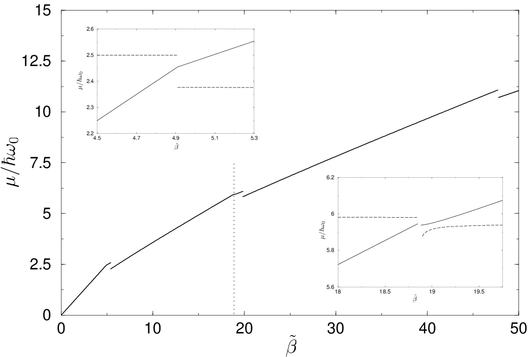
Figure 12: Chemical potential in units of ℏ​ω0\hbar\omega_{0} as a function of β~\tilde{\beta}. The dotted line indicates the transition between the states c) and d) (see text). The insets show the dependence μ~​(β~)\tilde{\mu}(\tilde{\beta}) in the vicinity of the quantum transitions at β~=4.9\tilde{\beta}=4.9 (upper inset) and at β~≃18.9\tilde{\beta}\simeq 18.9 (lower inset). The dashed lines in the insets indicate the derivative ∂μ~/∂β~\partial\tilde{\mu}/\partial\tilde{\beta} in arbitrary units.

The narrow channel geometry for rotating Bose gases was first considered in Ref. [14], where the roton-maxon structure of the excitations of the BEC without vortices has been found, and the phase diagram was presented with an emphasis on the first two transitions which can be calculated analytically. A numerical study of the related problem was done in Ref. [15], where corrugated states were discussed. However the analysis of quantum transitions in Ref. [15] stops at the appearance of the state with two vortex rows, although the states with up to 4 rows of vortices have also been observed. Here, we present a complete phase diagram and identify the nature of quantum phase transitions. The chemical potential as a function of β~\tilde{\beta} for β~<50\tilde{\beta}<50 is shown in Fig. 12, indicating three first order transitions, one second order transition, and the above described peculiar transition between the states c) and d).

The extension of the condensate wavefunction in the xx-direction increases with increasing the interaction strength, and the two-dimensional density decreases. This decreases the average filling factor defined as ν=N/Nv\nu=N/N_{v}. The Gross-Pitaevskii equation gives a good description in the limit of large filling factors and we expect our picture to break down at very large β~\tilde{\beta}. Eventually, when the number of particles becomes of the order of the number of vortices NvN_{v}, the vortex lattice melts through the phase transition to a strongly correlated state. The limiting case of extremely large β~\tilde{\beta} corresponds to the Laughlin state with ν=1/2\nu=1/2, and it was discussed for the narrow channel with periodic boundary conditions in the xx direction in Ref. [27].

V Conclusion

In conclusion, we found an analytical solution for the vortex lattice in a rapidly rotating BEC in the LLL. This solution is asymptotically exact in the limit of a very large number of vortices, and we discuss non-Thomas-Fermi effects in the density profile. The results are obtained for two limiting cases, circularly symmetric BEC and narrow channel geometry. In the latter case we present a complete phase diagram and identify the order of quantum phase transitions occurring under an increase in the interaction strength and/or rotation frequency and resulting in an increase in the number of vortex rows.

Acknowledgements

We are grateful to N.R. Cooper for helpful discussions. S.M. and S.O. acknowledge discussions with A. Aftalion, X. Blanc and F. Nier. This work was supported by ANR (Grants ANR-07-BLAN-0238 and ANR-08-BLAN-0165), by the IFRAF Institute, and by the Dutch Foundation FOM. G.S. wishes to thank the Aspen Center for Physics and the Institute for Nuclear Theory of the Univeresity of Washington for their hospitality/support during the workshop ”Quantum Simulation/Computation with Cold Atoms and Molecules” (Aspen, May-June, 2009) and the workshop ”From Femptoscience to Nanoscience: Nuclei, Quantum Dots, and Nanostructures” (Seattle, August, 2009), where part of the present work has been done. D.K. acknowledges support from EPSRC grant EP/D066379/1. LPTMS is a mixed research unit No.8626 of CNRS and Université Paris Sud.

Appendix

Let us give a detailed derivation of the projection of the Gross-Pitaevskii equation for a rapidly rotating Bose-condensed gas onto the lowest Landau level [28]. The gas is confined in an asymmetric harmonic potential V⁡(𝐫)=m⁡(ωx2​x2+ωy2​y2)/2V({\bf r})=m(\omega_{x}^{2}x^{2}+\omega_{y}^{2}y^{2})/2, and we assume without loss of generality that ωy<ωx\omega_{y}<\omega_{x}.

In the symmetric gauge the single-particle Hamiltonian is similar to that of equation (3):

H=12​(𝐩^−[𝛀×𝐫])2+12​(ωx2−Ω2)​x2+12​(ωy2−Ω2)​y2,H=\frac{1}{2}(\hat{\bf p}-[{\bf\Omega}\times{\bf r}])^{2}+\frac{1}{2}(\omega_{x}^{2}-\Omega^{2})x^{2}+\frac{1}{2}(\omega_{y}^{2}-\Omega^{2})y^{2}, (45)

where we put ℏ=m=1\hbar=m=1. Drawing an analogy with a charged particle in a uniform magnetic field BB, the rotation frequency Ω\Omega is identified with half the cyclotron frequency ωc\omega_{c}, and putting the particle charge and light velocity equal to unity we have Ω=ωc=B/2\Omega=\omega_{c}=B/2. In complex coordinates the Hamiltonian (45)rewrites as

H(z,z¯)=−2∂∂¯+ωc(z¯∂¯−z∂)+12ωt2zz¯+18(ωx2−ωy2)(z2+z¯2),H(z,\bar{z})=-2\partial\bar{\partial}+\omega_{c}(\bar{z}\bar{\partial}-z\partial)+\frac{1}{2}\omega_{t}^{2}z\bar{z}+\frac{1}{8}(\omega_{x}^{2}-\omega_{y}^{2})(z^{2}+\bar{z}^{2}), (46)

where ωt2=ωx2+ωy2\omega_{t}^{2}=\omega_{x}^{2}+\omega_{y}^{2} and can be rewritten as ωt2=ωc2+(ω~x2+ω~y2)/2\omega_{t}^{2}=\omega_{c}^{2}+(\tilde{\omega}_{x}^{2}+\tilde{\omega}_{y}^{2})/2, with ω~x2=ωx2−ωc2\tilde{\omega}_{x}^{2}=\omega_{x}^{2}-\omega_{c}^{2} and ω~y2=ωy2−ωc2\tilde{\omega}_{y}^{2}=\omega_{y}^{2}-\omega_{c}^{2}.

Introducing the frequencies ωt±=ωc2+(ω~x±ω~y2)2\omega_{t}^{\pm}=\sqrt{\omega_{c}^{2}+(\frac{\tilde{\omega}_{x}\pm\tilde{\omega}_{y}}{2})^{2}} and the dimensionless parameter ρ2=(ωt−+ωc)​(ωt++ωc)(ωt−−ωc)​(ωt+−ωc)\rho^{2}=\sqrt{\frac{(\omega_{t}^{-}+\omega_{c})(\omega_{t}^{+}+\omega_{c})}{(\omega_{t}^{-}-\omega_{c})(\omega_{t}^{+}-\omega_{c})}}, the unnormalized ground state wavefunction is

⟨z,z¯|Ψ0⟩=e−12​ωt+​z​z¯e−12​(a​z2+b​z¯2),\langle z,\bar{z}|\Psi_{0}\rangle=e^{-\frac{1}{2}\omega_{t}^{+}z\bar{z}}e^{-\frac{1}{2}(az^{2}+b\bar{z}^{2})}, (47)

where a=12​ρ2​(ωt−−ωc)a=\frac{1}{2}\rho^{2}(\omega_{t}^{-}-\omega_{c}), b=12​(ωt−+ωc)/ρ2b=\frac{1}{2}(\omega_{t}^{-}+\omega_{c})/{\rho^{2}}, and H⁡|Ψ0⟩=ωt+​|Ψ0⟩H|\Psi_{0}\rangle=\omega_{t}^{+}|\Psi_{0}\rangle.

The lowest Landau level in the asymmetric well is obtained by redefining |Ψ⟩=|Ψo​Ψ~⟩|\Psi\rangle=|\Psi_{o}\tilde{\Psi}\rangle and requiring the Hamiltonian H~\tilde{H} which acts on Ψ~⟩\tilde{\Psi}\rangle to depend only on a single variable representing a linear combination of zz and z¯\bar{z}:

u=z−1ρ2​z¯.u=z-\frac{1}{\rho^{2}}\bar{z}. (48)

The eigenvalue equation acting on |Ψ~⟩|\tilde{\Psi}\rangle then reads:

(E−ωt+)​Ψ~=2ρ2​Ψ~′′+(ωt+−ωt−)​u​Ψ~′.(E-\omega_{t}^{+})\tilde{\Psi}=\frac{2}{\rho^{2}}\tilde{\Psi}^{\prime\prime}+(\omega_{t}^{+}-\omega_{t}^{-})u\tilde{\Psi}^{\prime}. (49)

Let us define a dimensionless variable u′=i​ρ2​ωt+−ωt−​uu^{\prime}=i\frac{\rho}{2}\sqrt{\omega_{t}^{+}-\omega_{t}^{-}}\;u so that the eigenvalue equation (49) becomes

(E−ωt+)​Ψ~=ωt+−ωt−2​(−Ψ~′′+2​u′​Ψ~′)(E-\omega_{t}^{+})\tilde{\Psi}=\frac{\omega_{t}^{+}-\omega_{t}^{-}}{2}(-\tilde{\Psi}^{\prime\prime}+2u^{\prime}\tilde{\Psi}^{\prime}) (50)

This is a Hermite equation (ωt+>ωt−\omega_{t}^{+}>\omega_{t}^{-}) with eigenfunctions Ψ~n​(u′)=Hn​(u′)\tilde{\Psi}_{n}(u^{\prime})=H_{n}(u^{\prime}) such that

⟨z,z¯|Ψn⟩=NnHn(u′)Ψ0(z,z¯)\langle z,\bar{z}|\Psi_{n}\rangle=N_{n}H_{n}(u^{\prime})\Psi_{0}(z,\bar{z})

with eigenvalues

En=n⁡(ωt+−ωt−)+ωt+.E_{n}=n(\omega_{t}^{+}-\omega_{t}^{-})+\omega_{t}^{+}.

Introducing the quantity μ\mu:

cosh⁡μ=ωt−ωc​(ωt+−ωc)​(ωt++ωc)(ωt+−ωt−)​(ωt++ωt−)\cosh\mu=\frac{\omega_{t}^{-}}{\omega_{c}}\sqrt{\frac{(\omega_{t}^{+}-\omega_{c})(\omega_{t}^{+}+\omega_{c})}{(\omega_{t}^{+}-\omega_{t}^{-})(\omega_{t}^{+}+\omega_{t}^{-})}}
sinh⁡μ=ωt+ωc​(ωt−−ωc)​(ωt−+ωc)(ωt+−ωt−)​(ωt++ωt−)\sinh\mu=\frac{\omega_{t}^{+}}{\omega_{c}}\sqrt{\frac{(\omega_{t}^{-}-\omega_{c})(\omega_{t}^{-}+\omega_{c})}{(\omega_{t}^{+}-\omega_{t}^{-})(\omega_{t}^{+}+\omega_{t}^{-})}}

so that

⟨Ψo|z,z¯⟩⟨z,z¯|Ψo⟩=esinh⁡2​μ​(−u′​u¯′+12​tanh⁡μ⁡(u′2+u¯′2)),\langle\Psi_{o}|z,\bar{z}\rangle\langle z,\bar{z}|\Psi_{o}\rangle=e^{\sinh 2\mu(-u^{\prime}\bar{u}^{\prime}+\frac{1}{2}\tanh\mu(u^{\prime 2}+\bar{u}^{\prime 2}))},

and using the relation

∫d​u′​d​u¯′π​e−u′​u¯′+12​tanh⁡μ⁡(u′2+u¯′2)​Hl​(u′sinh⁡2​μ)​Hk​(u¯′sinh⁡2​μ)=cosh⁡μ​l!(tanh⁡μ2)l​δk,l,\int\frac{du^{\prime}d\bar{u}^{\prime}}{\pi}e^{-u^{\prime}\bar{u}^{\prime}+\frac{1}{2}\tanh\mu(u^{\prime 2}+\bar{u}^{\prime 2})}H_{l}({u^{\prime}\over\sqrt{\sinh 2\mu}})H_{k}({\bar{u}^{\prime}\over\sqrt{\sinh 2\mu}})=\cosh\mu{l!\over({\tanh\mu\over 2})^{l}}\delta_{k,l},

the normalization factor NnN_{n} is found to be

Nn=(−i)n​1π​n!​(tanh⁡μ2)n2​ωt+​ωt−ωc​1cosh⁡μ.N_{n}=(-i)^{n}{1\over\sqrt{\pi n!}}\bigg({\tanh\mu\over 2}\bigg)^{{n\over 2}}\sqrt{{\omega_{t}^{+}\omega_{t}^{-}\over\omega_{c}}{1\over\cosh\mu}}.

The projector onto the LLL of an asymmetric harmonic well, PL​L​L=∑n≥0|Ψn⟩​⟨Ψn|P_{LLL}=\sum_{n\geq 0}|\Psi_{n}\rangle\langle\Psi_{n}|, is

⟨z1,z¯1​|PL​L​L|​z2,z¯2⟩=ωt+​ωt−π​ωc​cosh⁡μ​e−12​(a​z12+b​z¯12+ωt+​z1​z¯1)​e−12​(a​z¯22+b​z22+ωt+​z2​z¯2)\displaystyle\langle z_{1},\bar{z}_{1}|P_{LLL}|z_{2},\bar{z}_{2}\rangle={\omega_{t}^{+}\omega_{t}^{-}\over\pi\omega_{c}\cosh\mu}e^{-{1\over 2}(az_{1}^{2}+b\bar{z}_{1}^{2}+\omega_{t}^{+}z_{1}\bar{z}_{1})}e^{-{1\over 2}(a\bar{z}_{2}^{2}+bz_{2}^{2}+\omega_{t}^{+}z_{2}\bar{z}_{2})}
∑n≥0(tanh⁡μ2)n​1n!​Hn​(u1′)​Hn​(u¯2′).\displaystyle\sum_{n\geq 0}\bigg({\tanh\mu\over 2}\bigg)^{n}{1\over\ n!}H_{n}(u_{1}^{\prime})H_{n}(\bar{u}_{2}^{\prime}). (51)

Using the relation

Hn​(u′)=2nπ​∫−∞∞(u′+i​t)n​e−t2​𝑑tH_{n}(u^{\prime})={2^{n}\over\sqrt{\pi}}\int_{-\infty}^{\infty}(u^{\prime}+it)^{n}e^{-t^{2}}dt

one obtains

⟨z1,z¯1​|PL​L​L|​z2,z¯2⟩=ωt+​ωt−π​ωc​e−12​(a​z12+b​z¯12+ωt+​z1​z¯1)​e−12​(a​z¯22+b​z22+ωt+​z2​z¯2)\displaystyle\langle z_{1},\bar{z}_{1}|P_{LLL}|z_{2},\bar{z}_{2}\rangle={\omega_{t}^{+}\omega_{t}^{-}\over\pi\omega_{c}}e^{-{1\over 2}(az_{1}^{2}+b\bar{z}_{1}^{2}+\omega_{t}^{+}z_{1}\bar{z}_{1})}e^{-{1\over 2}(a\bar{z}_{2}^{2}+bz_{2}^{2}+\omega_{t}^{+}z_{2}\bar{z}_{2})}
e−sinh2⁡μ⁡(u1′2+u¯2′2)+sinh⁡2​μ​u1′​u¯2′.\displaystyle e^{-\sinh^{2}\mu(u_{1}^{\prime 2}+\bar{u}_{2}^{\prime 2})+\sinh 2\mu u_{1}^{\prime}\bar{u}_{2}^{\prime}}. (52)

Any state |ΨL​L​L⟩=PL​L​L​|Ψ⟩|\Psi_{LLL}\rangle=P_{LLL}|\Psi\rangle in the LLL is a linear combination of LLL eigenstates:

⟨z,z¯|ΨL​L​L⟩=∑n=0∞cn⟨z,z¯|Ψn⟩=f(u′)e−12​(a​z2+b​z¯2+ωt+​z​z¯)\langle z,\bar{z}|\Psi_{LLL}\rangle=\sum_{n=0}^{\infty}c_{n}\langle z,\bar{z}|\Psi_{n}\rangle=f(u^{\prime})e^{-{1\over 2}(az^{2}+b\bar{z}^{2}+\omega_{t}^{+}z\bar{z})}

where f⁡(u′)f(u^{\prime}) is an analytic function.

Consider now the Hamiltonian (46) to which we add a scalar potential V⁡(z,z¯)V(z,\bar{z}):

H(z,z¯)=−2∂∂¯+ωc(z¯∂¯−z∂)+12ωt2zz¯+18(ωx2−ωy2)(z2+z¯2)+V(z,z¯)H(z,\bar{z})=-2\partial\bar{\partial}+\omega_{c}(\bar{z}\bar{\partial}-z\partial)+\frac{1}{2}\omega_{t}^{2}z\bar{z}+\frac{1}{8}(\omega_{x}^{2}-\omega_{y}^{2})(z^{2}+\bar{z}^{2})+V(z,\bar{z}) (53)

Projecting the eigenvalue equation H​|Ψ⟩=E​|Ψ⟩H|\Psi\rangle=E|\Psi\rangle onto the LLL amounts to ⟨z1,z¯1​|PL​L​L​H​PL​L​L|​Ψ⟩=E⁡⟨z1,z¯1​|PL​L​L|​Ψ⟩\langle z_{1},\bar{z}_{1}|P_{LLL}HP_{LLL}|\Psi\rangle=E\langle z_{1},\bar{z}_{1}|P_{LLL}|\Psi\rangle. This gives

ωt+​ωt−π​ωc​∫d​z2​d​z¯2​e−12​(a​z¯22+b​z22+ωt+​z2​z¯2)​e−12​(a​z22+b​z¯22+ωt+​z2​z¯2)​e−sinh2⁡μ⁡(u1′2+u¯2′2)+sinh⁡2​μ​u1′​u¯2′\displaystyle{\omega_{t}^{+}\omega_{t}^{-}\over\pi\omega_{c}}\int dz_{2}d\bar{z}_{2}e^{-{1\over 2}(a\bar{z}_{2}^{2}+bz_{2}^{2}+\omega_{t}^{+}z_{2}\bar{z}_{2})}e^{-{1\over 2}(az_{2}^{2}+b\bar{z}_{2}^{2}+\omega_{t}^{+}z_{2}\bar{z}_{2})}e^{-\sinh^{2}\mu(u_{1}^{\prime 2}+\bar{u}_{2}^{\prime 2})+\sinh 2\mu u_{1}^{\prime}\bar{u}_{2}^{\prime}}
H⁡(z2,z¯2)​f​(u2′)=E​f​(u1′).\displaystyle H(z_{2},\bar{z}_{2})f(u_{2}^{\prime})=Ef(u_{1}^{\prime}). (54)

Writing explicitly H⁡(z2,z¯2)H(z_{2},\bar{z}_{2}) and changing the integration variables to u2′,u¯2′u^{\prime}_{2},\bar{u}^{\prime}_{2}, we have

sinh⁡2​μπ​e−sinh2⁡μ​u1′2​∫d​u2′​d​u¯2′​esinh2⁡μ​u2′2​esinh⁡2​μ​(u1′​u¯2′−u2′​u¯2′)\displaystyle{\sinh 2\mu\over\pi}e^{-\sinh^{2}\mu u_{1}^{\prime 2}}\int du_{2}^{\prime}d\bar{u}_{2}^{\prime}e^{\sinh^{2}\mu u_{2}^{\prime 2}}e^{\sinh 2\mu(u_{1}^{\prime}\bar{u}_{2}^{\prime}-u_{2}^{\prime}\bar{u}_{2}^{\prime})}
(ωt+−ωt−2​(−f′′​(u2′)+2​u2′​f′​(u2′))+ωt+​f​(u2′)+V⁡(u2′,u¯2′)​f​(u2′))=E​f​(u1′).\displaystyle\bigg({\omega_{t}^{+}-\omega_{t}^{-}\over 2}(-f^{\prime\prime}(u_{2}^{\prime})+2u_{2}^{\prime}f^{\prime}(u_{2}^{\prime}))+\omega_{t}^{+}f(u_{2}^{\prime})+V(u_{2}^{\prime},\bar{u}_{2}^{\prime})f(u_{2}^{\prime})\bigg)=Ef(u_{1}^{\prime}). (55)

Using the Bargman identity

sinh⁡2​μπ​∫d​u2′​d​u¯2′​esinh⁡2​μ​(u¯2′​u1′−u2′​u¯2′)​f​(u2′)=f⁡(u1′),{\sinh 2\mu\over\pi}\int du_{2}^{\prime}d\bar{u}_{2}^{\prime}e^{\sinh 2\mu(\bar{u}_{2}^{\prime}u_{1}^{\prime}-u_{2}^{\prime}\bar{u}_{2}^{\prime})}f(u_{2}^{\prime})=f(u_{1}^{\prime}),

one finally obtains

(E−ωt+)f(u′)=ωt+−ωt−2(−f′′(u′)+2u′f′(u′))+e−sinh2⁡μ​u′2:V(u′,1sinh⁡2​μ∂u′):esinh2⁡μ​u′2f(u′),(E-\omega_{t}^{+})f(u^{\prime})={\omega_{t}^{+}-\omega_{t}^{-}\over 2}(-f^{\prime\prime}(u^{\prime})+2u^{\prime}f^{\prime}(u^{\prime}))+e^{-\sinh^{2}\mu u^{\prime 2}}:V(u^{\prime},{1\over\sinh 2\mu}\partial_{u^{\prime}}):e^{\sinh^{2}\mu u^{\prime 2}}f(u^{\prime}),

where the notation :V(u′,1sinh⁡2​μ∂u′)::V(u^{\prime},{1\over\sinh 2\mu}\partial_{u^{\prime}}): means that in V⁡(u′,u¯′)V(u^{\prime},\bar{u}^{\prime}) the variable u¯′\bar{u}^{\prime} has been replaced by the operator 1sinh⁡2​μ∂u′{1\over\sinh 2\mu}\partial_{u^{\prime}} and the normal ordering has been made. In the case of the Gross-Pitaevskii equation the scalar potential is replaced by the non-linear term

g⁡⟨ΨL​L​L|ΨL​L​L⟩=g​f​(u′)​f​(u¯′)​e−sinh⁡2​μ​u′​u¯′+sinh2⁡μ⁡(u′2+u¯′2)g\langle\Psi_{LLL}|\Psi_{LLL}\rangle=gf(u^{\prime})f(\bar{u}^{\prime})e^{-\sinh 2\mu u^{\prime}\bar{u}^{\prime}+\sinh^{2}\mu(u^{\prime 2}+\bar{u}^{\prime 2})}

so that Eq. (55) becomes

(E−ωt+)​f​(u1′)=ωt+−ωt−2​(−f′′​(u1′)+2​u1′​f′​(u1′))+\displaystyle(E-\omega_{t}^{+})f(u^{\prime}_{1})=\frac{\omega_{t}^{+}-\omega_{t}^{-}}{2}(-f^{\prime\prime}(u^{\prime}_{1})+2u^{\prime}_{1}f^{\prime}(u^{\prime}_{1}))+
g​sinh⁡2​μπ​e−sinh2⁡μ​u1′2​∫d​u2′​d​u¯2′​e2​sinh2⁡μ​u2′2+sinh2⁡μ​u¯2′2​e2​sinh⁡2​μ​(u¯′2​u1′/2−u2′​u¯′2)​f2​(u2′)​f​(u¯′2).\displaystyle g\frac{\sinh 2\mu}{\pi}e^{-\sinh^{2}{\mu u_{1}^{\prime}}^{2}}\int du_{2}^{\prime}d\bar{u}_{2}^{\prime}e^{2\sinh^{2}\mu{u_{2}^{\prime}}^{2}+\sinh^{2}{\mu\bar{u}_{2}^{\prime}}^{2}}e^{2\sinh 2\mu({\bar{u}^{\prime}}_{2}u^{\prime}_{1}/2-u^{\prime}_{2}{\bar{u}^{\prime}}_{2})}f^{2}(u^{\prime}_{2})f({\bar{u}^{\prime}}_{2}). (56)

Eq.(56) is a general form of the non-linear Gross-Pitaevskii equation projected onto the LLL of an asymmetric harmonic trap.

Let us now concentrate on the two cases of interest, circularly symmetric geometry and narrow channel geometry. In the symmetric geometry we have ωx=ωy=ω=ωt\omega_{x}=\omega_{y}=\omega=\omega_{t}, and ωt+−ωt−→ωt−ωc\omega_{t}^{+}-\omega_{t}^{-}\to\omega_{t}-\omega_{c},

sinh⁡μ→ωt2​ωc​ω​(ω~x−ω~y)→0,cosh⁡μ→1\sinh\mu\to{\omega_{t}\over 2\omega_{c}\omega}(\tilde{\omega}_{x}-\tilde{\omega}_{y})\to 0,\quad\cosh\mu\to 1
−2​i​u′→ωt−ωc​ρ​z-2iu^{\prime}\to\sqrt{\omega_{t}-\omega_{c}}\rho z
ρ→2​ω​ωc(ωt−ωc)​(ω~x−ω~y)→∞\rho\to 2\sqrt{{\omega\omega_{c}\over(\omega_{t}-\omega_{c})(\tilde{\omega}_{x}-\tilde{\omega}_{y})}}\to\infty

so that

u′→i​ω​ωcω~x−ω~y​z→i​∞.u^{\prime}\to i\sqrt{{\omega\omega_{c}\over\tilde{\omega}_{x}-\tilde{\omega}_{y}}}z\to i\infty.

Changing variables, u′→zu^{\prime}\to z, equation (56) reduces to

(ωt−ωc)​z1​f′​(z1)+g​ωtπ​∫d​z2​d​z¯2​e2​ωt​(z¯2​z1/2−z2​z¯2)​f2​(z2)​f​(z¯2)=(E−ωt)​f​(z1).(\omega_{t}-\omega_{c})z_{1}f^{\prime}(z_{1})+g{\omega_{t}\over\pi}\int dz_{2}d\bar{z}_{2}e^{2\omega_{t}(\bar{z}_{2}z_{1}/2-z_{2}\bar{z}_{2})}f^{2}(z_{2})f(\bar{z}_{2})=(E-\omega_{t})f(z_{1}). (57)

Finally, when ω→0\omega\to 0 (critical rotation), i.e. ωt→ωc\omega_{t}\to\omega_{c}, (57) becomes

g​ωcπ​∫d​z2​d​z¯2​e2​ωc​(z¯2​z1/2−z2​z¯2)​f2​(z2)​f​(z¯2)=(E−ωc)​f​(z1).g{\omega_{c}\over\pi}\int dz_{2}d\bar{z}_{2}e^{2\omega_{c}(\bar{z}_{2}z_{1}/2-z_{2}\bar{z}_{2})}f^{2}(z_{2})f(\bar{z}_{2})=(E-\omega_{c})f(z_{1}). (58)

Putting ωt=ω\omega_{t}=\omega, ωc=Ω\omega_{c}=\Omega, (E−ωt)=μ~(E-\omega_{t})=\tilde{\mu}, and f→(N/l~)​ff\rightarrow(\sqrt{N}/\tilde{l})f in Eq. (57), we obtain Eq. (9).

In the narrow channel geometry ω~y→0\tilde{\omega}_{y}\to 0, and ωt+−ωt−→ω~x​ω~y/(2​ωc)\omega_{t}^{+}-\omega_{t}^{-}\to{\tilde{\omega}_{x}\tilde{\omega}_{y}/(2\omega_{c})}

sinh⁡μ=cosh⁡μ→ωt′​(ωt′2−ωc2)ωc​ω~x​ω~y\sinh\mu=\cosh\mu\to\sqrt{{{{\omega^{\prime}_{t}}}({{\omega^{\prime}_{t}}}^{2}-\omega_{c}^{2})\over\omega_{c}\tilde{\omega}_{x}\tilde{\omega}_{y}}}
−2​i​u′→ω~x​ω~y2​ωc​ρ​u-2iu^{\prime}\to\sqrt{{\tilde{\omega}_{x}\tilde{\omega}_{y}\over 2\omega_{c}}}\rho u
ρ→ωt′+ωcωt′−ωc\rho\to\sqrt{{{{\omega^{\prime}_{t}}}+\omega_{c}\over{{\omega^{\prime}_{t}}}-\omega_{c}}}

where ωt′=ωc2+ω~x24{\omega^{\prime}_{t}}=\sqrt{\omega_{c}^{2}+{\tilde{\omega}_{x}^{2}\over 4}}. Changing variables, u′→u=z−z¯/ρ2u^{\prime}\to u=z-\bar{z}/\rho^{2}, equation (56) reduces to

2​ωt′−ωcωt′+ωc​f′′​(u1)+g​ωt′′π​eωt′′​u12/2​∫d​u2​d​u¯2​e−ωt′′​(u22+u¯22/2)​e2​ωt′′​(u¯2​u1/2−u¯2​u2)​f2​(u2)​f​(u¯2)=(E−ωt′)​f​(u1),2{{{\omega^{\prime}_{t}}}-\omega_{c}\over{{\omega^{\prime}_{t}}}+\omega_{c}}f^{\prime\prime}(u_{1})+g{{{\omega^{\prime\prime}_{t}}}\over\pi}e^{{{\omega^{\prime\prime}_{t}}}u_{1}^{2}/2}\int du_{2}d\bar{u}_{2}e^{-{{\omega^{\prime\prime}_{t}}}(u_{2}^{2}+{\bar{u}_{2}}^{2}/2)}e^{2{{\omega^{\prime\prime}_{t}}}(\bar{u}_{2}u_{1}/2-\bar{u}_{2}u_{2})}f^{2}(u_{2})f(\bar{u}_{2})=(E-{{\omega^{\prime}_{t}}})f(u_{1}), (59)

where ωt′′=ωt′​(ωt′+ωc2​ωc)2{{\omega^{\prime\prime}_{t}}}={{\omega^{\prime}_{t}}}({{{\omega^{\prime}_{t}}}+\omega_{c}\over 2\omega_{c}})^{2}. Turning to the variable ζ=i​ωt′′​u2\zeta=i\sqrt{\omega^{\prime\prime}_{t}}u_{2} , putting ωc=Ω\omega_{c}=\Omega, and noticing that ωt′=Ω~\omega^{\prime}_{t}=\tilde{\Omega} where Ω~\tilde{\Omega} was defined in Section III, we have 2​ωt′′​(ωt′−ωc)/(ωt′+ωc)=ω02\omega^{\prime\prime}_{t}(\omega^{\prime}_{t}-\omega_{c})/(\omega^{\prime}_{t}+\omega_{c})=\omega_{0}, with ω0\omega_{0} introduced in Eq. (34). Then, after rescaling the function ff as f→(N/l~)​ff\rightarrow(\sqrt{N}/\tilde{l})f, equation (59) transforms into Eq. (34).

References

  • [1] See for review: N. R. Cooper, Advances in Physics 57, 539 (2008).
  • [2] See for review: A. L. Fetter, Rev. Mod. Phys. 81, 647 (2009).
  • [3] Tin-Lun Ho, Phys. Rev. Lett. 87, 060403 (2001).
  • [4] D.A. Butts and D.S. Rokhsar, Nature 397, 327 (1999).
  • [5] N.R. Cooper, S. Komineas, and N. Read, Phys. Rev. A 70, 033604 (2004).
  • [6] I. Coddington, P. C. Haljan, P. Engels, V. Schweikhard, S. Tung, and E. A. Cornell, Phys. Rev. A 70, 063607 (2004).
  • [7] A. Aftalion, X. Blanc, J. Dalibard, Phys. Rev. A 71, 023611 (2005).
  • [8] P. Rosenbusch, D.S. Petrov, S. Sinha, F. Chevy, V. Bretin, Y. Castin, G.V. Shlyapnikov, and J. Dalibard, Phys. Rev. Lett. 88, 250403 (2002).
  • [9] A. L. Fetter, Phys. Rev. A 75, 013620 (2007).
  • [10] M. Linn, M. Niemeyer, and A.L. Fetter, Phys. Rev. A 64, 023602 (2001).
  • [11] M.O. Oktel, Phys. Rev. A 69, 023618 (2004).
  • [12] A. Aftalion, X. Blanc and F. Nier, Phys. Rev. A 73, 011601(R) (2006).
  • [13] A. Aftalion, X. Blanc and N. Lerner, arXiv:0804.0971.
  • [14] S. Sinha and G.V. Shlyapnikov, Phys. Rev. Lett. 94, 150401 (2005).
  • [15] P. Sanchez-Lotero and J. J. Palacios, Phys. Rev. A 72, 043613 (2005).
  • [16] D.S. Petrov, M. Holzmann, and G.V. Shlyapnikov, Phys. Rev. Lett. 84, 2551 (2000).
  • [17] R.A. Smith and N.K.Wilkin, Phys. Rev. A 62, 061602(R) (2000).
  • [18] N.R. Cooper, N.K. Wilkin, and J.M.F. Gunn, Phys. Rev. Lett. 87, 120405 (2001).
  • [19] B. Paredes, P. Fedichev, J.I. Cirac, and P. Zoller, Phys. Rev. Lett. 87, 010402 (2001).
  • [20] N. Regnault, Th. Jolicoeur, Phys. Rev. B 69, 235309 (2004).
  • [21] S. Mashkevich, S. Matveenko and S. Ouvry, Nucl. Phys. B[FS] 763 (2007) 431.
  • [22] v. Bargmann, Comm. Pure Appl. Math. 14, 187 (1961); Rev. Mod. Phys. 34, 829 (1962).
  • [23] S. M. Girvin and T. Jach, Phys. Rev. B, 29, 5617 (1984).
  • [24] C. Foot, private communication.
  • [25] M. Abramowitz and I. A. Stegun, Handbook of Mathematical Functions (Dover, New York, 1966).
  • [26] S. Kirkpatrick, C.D. Gelatt Jr., and M.P. Vecchi, Science 220, 671 (1983).
  • [27] E. H. Rezayi, F. D. M. Haldane, Phys. Rev. B 50, 17199 (1994).
  • [28] The projected Gross-Pitaevskii equation leads to the same results as the ones obtained by using the initial equation, with the condensate wavefunction representing a linear superposition of LLL eigenstates [4, 5, 7, 9, 11, 12].