Self-force with (3+1) codes: a primer for numerical relativists
Abstract
Prescriptions for numerical self-force calculations have traditionally been designed for frequency-domain or (1+1) time-domain codes which employ a mode decomposition to facilitate in carrying out a delicate regularization scheme. This has prevented self-force analyses from benefiting from the powerful suite of tools developed and used by numerical relativists for simulations of the evolution of comparable-mass black hole binaries. In this work, we revisit a previously-introduced (3+1) method for self-force calculations, and demonstrate its viability by applying it to the test case of a scalar charge moving in a circular orbit around a Schwarzschild black hole. Two (3+1) codes originally developed for numerical relativity applications were independently employed, and in each we were able to compute the two independent components of the self-force and the energy flux correctly to within . We also demonstrate consistency between -component of the self-force and the scalar energy flux. Our results constitute the first successful calculation of a self-force in a (3+1) framework, and thus open opportunities for the numerical relativity community in self-force analyses and the perturbative modeling of extreme-mass-ratio inspirals.
pacs
04.25.D-,04.25.dg,04.25.Nx,04.20.Cv,04.30.DbI Introduction
A pressing challenge in gravitational wave source modeling is the inspiral of a solar mass compact object into a supermassive black hole, better known as an extreme-mass-ratio inspiral or EMRI. These inspirals result from scattering processes in the star-rich cores of galaxies, and tend to be highly-eccentric in the strong field region of the supermassive black hole [1]. The intricate gravitational waves they emit are believed to be the most complicated among LISA sources, and their detection and analysis promise significant science returns for relativistic astrophysics and general relativity [2]. For this to come to fruition, precise models of their gravitational waves will be necessary.
Immediately confronting this objective are the dramatically different scales that characterize EMRIs. First, there is the short length scale of the distortion on the background spacetime made by the compact object, which will need to be resolved well enough. Then, there is the large length scale of the supermassive black hole, which sets the distance to the wavezone, where the gravitational wave signal is to be extracted. Finally, since a typical EMRI source for LISA will make about orbits, long-term evolutions will be required to produce gravitational wave templates of use to data analysis. These considerations conspire to make EMRI modeling a difficult problem for numerical relativity.
At some point, the steady advance of computational technology will allow the numerical relativity community to tackle the full dynamics of this binary system. In the meantime it seems prudent to develop approximate schemes that will reliably produce templates of adequate accuracy. One such scheme takes advantage of the small mass-ratio (say ) and treats the problem in a perturbative fashion. At lowest order, the system is but an infinitesimal test mass moving in a black hole spacetime, for which we know the motion to be geodesic in that spacetime. For such a case, the mature formalism of black hole perturbation theory is able to accurately calculate first-order metric perturbations, from which one infers gravitational waveforms. The foundations for these sorts of calculations [3, 4, 5] were laid out beginning over fifty years ago. However, the accuracy requirements of LISA, particularly on the phase of the waveform throughout the entire mission lifetime, demand that our models go beyond this leading order case. (An instructive scaling argument can be found in Sec. 11.1 of [6]). One thus has to consistently take into account next-to-leading order effects on the motion of the particle and the waveform. From this perspective, the dynamics of the inspiral are viewed as the motion of a finite (but small) point mass in a background black hole spacetime. The goal is then to determine these finite-mass effects on both the motion of the point mass and the corresponding gravitational waveform.
These effects are attributed to the self-force; the dissipative part of which is the more familiar phenomenon of radiation reaction. For a point mass moving in flat spacetime, this effect is entirely local. Only emission at a given instant affects the motion of the particle at that same instant. In curved spacetime, due to scattering with the curvature, the motion of the particle is affected by fields it gave rise to in its causal past. This makes the resulting physics much richer than of the flat spacetime case. The same scenario also applies to scalar and electric charged particles moving in curved spacetime. While often interesting in their own right, these also serve as useful and technically less-demanding toy problems for testing new methods and techniques.
The effect of the self-force is a small acceleration on the point mass resulting in a secular deviation away from what would otherwise have been geodesic motion in the background spacetime. This self-force will need to be calculated and used to modify the motion of the point mass as often as is practical throughout the course of the inspiral. Formal expressions for this self-force given in terms of an integral over the particle’s entire past history have been ironed out in the literature [7, 8, 9], but these are hardly convenient for practical calculations. The challenge is then to come up with an efficient way to compute self-forces based on these formal expressions. Several useful prescriptions have been developed to address this issue [10, 11], but most influential of these is the mode-sum prescription [12, 13, 14], which we shall describe below.
An alternative viewpoint of the self-force scenario is that instead of a backreacting “force” accelerating the point mass in the background spacetime, the motion of the point mass is really geodesic motion on the distorted background geometry [15, 6]. In this framework, the task is to determine the appropriate distorted geometry upon which to impose geodesic motion (or equivalently, the correct smooth potentials governing the motion of scalar and electric charges). The procedure thus involves first computing the metric perturbation induced by the point mass on the background spacetime metric (which would be divergent at the location of the point mass), and then appropriately regularizing this metric perturbation to give the correct smooth perturbation . The motion of the point mass will then be geodesic motion in the perturbed spacetime .
This perspective has been useful on both theoretical and practical fronts. Most notably, it has reconciled the notion of a self-force with our understanding of the equivalence principle [15]. It has also served as the basis of convenient variants of the original mode-sum prescription [16, 17, 18, 19, 20, 21, 22, 23, 24], and has thus advanced our understanding of this important calculational technique. The method presented in this manuscript is another off-shoot of this alternative viewpoint.
Much progress has been made in the calculation of the self-force on a charge that moves momentarily along some prescribed geodesic of the background spacetime. In particular, the mode-sum paradigm has contributed tremendously to our understanding of the elements of a self-force calculation and continues to serve as the conceptual backdrop upon which all other calculational schemes are to be understood. It has now been employed to evaluate the self-force or self-force effects in a variety of contexts – scalar [25, 16, 20, 17, 18, 19, 21, 22], electromagnetic [26], and gravitational [24, 27, 28] – for point sources moving along geodesics in a Schwarzschild background. Results for the Kerr spacetime are rare. The first calculation of a self force on a scalar charge moving through this background has been achieved only recently [29]. Despite this good progress, however, little has been done to achieve a dynamic calculation of the self-force that is then used to implement backreaction on moving point sources.
One of the reasons for this is that computing a self-force is a complicated process. A typical mode-sum calculation first requires a decomposition of the problem (i.e. fields and sources) into modes with, say, spherical or spheroidal harmonics. This is done in order to avoid having to handle the divergence in the physical retarded field numerically. Each mode component of the retarded field turns out to be finite at the location of the charge, and thus, numerically accessible. It is the sum of these modes that diverges. Buried in each mode is the piece that actually contributes to the self-force. The central insight of the mode-sum prescription is a way to access this relevant piece, based on an asymptotic analysis of the divergence in the retarded field. In calculating the self-force then, each computed mode is appropriately regularized (using an analytic expression determined by the asymptotic analysis) to leave the piece that contributes to the self-force. The regularized pieces are then summed to get the full self-force. Convergence of this sum is typically slow, going as , where is the maximum mode number, and is determined by the degree to which one analytically characterizes the asymptotic behavior of the divergent physical fields.
In [23] (henceforth referred to as Paper I), we introduced a method for calculating the self-force designed principally to obviate the apparent necessity of a decomposition into modes in order to perform the regularization of the retarded field. Through this alternative method, we proposed a (3+1) approach to self-force calculations, which fits squarely with the expertise and infrastructure found in the numerical relativity community. Our technique is reviewed in better detail below. Its core idea, however, is straightforward: rather than regularizing the retarded field, one can instead appropriately regularize the source term in the field equation from the start, and thus have the evolution codes deal with sufficiently-differentiable fields and sources that require no further regularization. In other words, we deal with regularization not as a post-processing step, but as preliminary work that needs to be performed before any numerical run. This work consists of appropriately replacing the delta-function representation of a point mass source by a regularized effective source. Designing this effective source for the wave equation can be done in such a way that a numerical evolution yields a differentiable field whose gradient at the location of the particle automatically gives the full self-force. In addition, this resulting regular field is such that it becomes the physical retarded solution in the wavezone, from which fluxes and the all-important waveforms can be extracted.
Two important features of this approach stand out. First, the evolution code never has to deal with divergent quantities (though the fields and sources are of finite differentiability); and second, both self-force calculation and waveform extraction are trivial, with accuracies limited chiefly by the accuracy that can be provided by the evolution code. It is these two features that call out to the numerical relativity community at large, for in effect all that is required for a self-force calculation is a (3+1) code that can accurately evolve wave equations with sources of limited differentiability. The ease with which one calculates a self-force in this approach suggests no significant impediment to implementing backreaction on the particle.
The idea of finding a good substitute for the delta function source in the context of self-force calculations is also being pursued by others in similar ways [30, 31, 32]. Barack and Golbourn [30] introduced a technique consisting of an -mode (azimuthal mode) regularization of the delta function source. Their regularization is also guided by analysis of the singular behavior of the retarded field at the location of the particle. First one solves (2+1) wave equations with regularized sources, then extracts the contribution to the self-force due to each azimuthal mode, and finally sums these to get the full self-force. Their approach is similar to ours in that it provides a way of representing point sources on a grid, but in keeping with the general strategy of the original mode-sum procedure (which was an -mode sum), it is likely to inherit some of the properties our approach seeks to overcome.
A new approach to evaluating the retarded field by Cañizares and Sopuerta [32] splits the problem into inner and outer domains marked by the location of the point charge. They situate the point source along the boundary shared by both domains, and then just impose appropriate jump conditions on the fields that cross the boundary. With the benefit of having to deal with only smooth fields, this method takes advantage of the exponential convergence of a pseudospectral implementation for evaluating the retarded field. In calculating a self-force, however, they are still restricted to performing a mode-sum of what remains after regularizing the output of their evolution code. A chief advantage of our method is precisely the fact that it escapes the requirement of a mode decomposition.
In Paper I, we reported an implementation of our method using a time-domain (1+1) code to compute the self-force and retarded field in the wavezone. By first breaking into modes, this implementation ran counter to the very motivations underlying our technique. This was done, however, mainly to provide a quick proof-of-principle, and to establish a more direct connection with more familiar approaches to self-force calculation.
In this work, we report for the first time on the feasibility of our technique in its intended setting. As a result, we have achieved the first calculation of a self-force in a (3+1) framework. Two different codes [33, 34] were employed in the implementation of our method, both originally intended for numerical relativity applications. As in Paper I, we focus on the simplest possible strong-field scenario involving a scalar point charge interacting with its own scalar field while in a circular orbit around a Schwarzschild black hole. In choosing to deal with this simple case, we also intend for this document to be a self-force primer and an invitation to numerical relativists who are on the lookout for new challenges. The insights gained from self-force analyses should prove useful to those wishing to tackle the extreme-mass-ratio regime of black hole binaries.
Outline and notation
Section II describes our formalism for replacing a point-particle delta-function source in a standard field equation with a particular abstract effective source. The effect is that not only does the resulting field equal the usual retarded field in the wave zone, but also the field is finite and differentiable at the particle. This allows it to be used directly in calculating the self-force acting on the particle. Some details regarding the effective source are given in Sect. III.
We describe a practical test application for our approach to self-force computations in Sect. IV. This test application has been previously well studied by the self-force community by using more traditional self-force techniques which are not particularly adaptable to numerical relativity [16, 17, 18, 19].
Section V contains the implementation details of modifications, with an eye on applications to self-force problems, of two different previously developed numerical relativity projects.
Details of the results following from the applications of these two codes to our test are given in Sect. VI. We compare the time and the radial components of the self-force, calculated by our two independent codes, with each other and with very accurate (but tediously obtained) well-known frequency-domain results [16, 17, 18, 19]. The time component of the self-force removes energy from the particle, and we also check its consistency with the energy flux via radiation down the black hole and out at infinity.
Section VII gives a summary of the apparent strengths and weaknesses of our effective source method for regularizing self-force problems. In very general terms we describe how currently available computer codes might be adapted specifically to self-force problems.
We have three appendices. Appendix A gives a 1+1D example of applying traditional finite differencing operators to a wave equation where the source is of limited differentiability. This elucidates the discussion of convergence. In Appendix B we derive the relationship between between the time component of the self-force and the radiative energy-flux into the black hole and out at infinity, in the case of a circular orbit and a scalar field. And we describe a very elementary, illustrative flat-space toy problem in Appendix C which demonstrates how a problem involving a delta-function point source can be transformed into one with a smooth source in a mathematically precise way.
For our tensor notation, we denote regular four-dimensional space time-time indices with letters taken from the first third of the alphabet , indices which are purely spatial in character are taken from the middle third, and indices from the last third and also and are associated with particular coordinate components. The operator is the covariant derivative operator compatible with the metric at hand. Partial derivatives with respect to are denoted , and with respect to a generic spatial coordinate by .
For the Schwarzschild metric, we use a coordinate system introduced by Eddington [35] and commonly known as Kerr-Schild coordinates to describe a Schwarzschild black hole.
Our use of the 3+1 formalism follows York [36] in all aspects except his labels for tensor indices.
II Field regularization for a scalar charge
In this section we review the discussion of our method found in Paper I. We shall discuss it for the case of a scalar point charge moving in curved spacetime. A typical self-force computation first involves solving the minimally-coupled scalar wave equation with a point charge source,
| (1) |
for the retarded field . Here is the derivative operator associated with the metric of the background spacetime and is the world line of the charge defined by and parameterized by the proper time . The physical solution of the resulting wave equation will be a retarded field that is singular at the location of the point charge. A formal expression for the self-force given by
| (2) |
would thus be undefined without a proper regularization prescription. Early analyses [37, 7, 8] were based upon a Hadamard expansion of the Green function, and showed that for a particle moving along a geodesic the self-force could be described in terms of the particle interacting only with the “tail” part of , which is finite at the particle itself. The mode-sum prescription is effectively a way of regularizing the righthand side of Eq. (2) to retrieve the force due to this tail part. Later [15] it was realized that a singular part of the field which exerts no force on the particle itself could be identified as an actual solution to Eq. (1) in a neighborhood of the particle. A formal description of in terms of parts of the retarded Green’s function is possible, but generally there is no exact functional description for in a neighborhood of the particle. Fortunately, as is shown in [16], an intuitively satisfying description for results from a careful expansion about the location of the particle:
| (3) |
where is a constant length scale of the background geometry and is a scalar field which simply satisfies in a very special Minkowski-like locally inertial coordinate system centered on the particle, first described by Thorne, Hartle and Zhang [38, 39] and applied to self-force problems in Refs. [40, 16, 6]. A detailed discussion of these coordinates can be found in [16, 6] and Appendix A of Paper I. Not surprisingly the singular part of the field, which exerts no force on the particle itself, appears as approximately the Coulomb potential to a local observer moving with the particle.
Our proposal for solving Eq. (1), and determining the self-force acting back on the particle now appears elementary. First we define
| (4) |
as a specific approximation to . By construction, we know that is singular at the particle and is elsewhere. Also, within a neighborhood of the world line of the particle
| (5) | |||||
It must be pointed out that for Eqs. (3) and (5) to be valid, the Thorne-Hartle-Zhang (THZ) coordinates must be known correctly to . Knowing the THZ coordinates only to would spoil the remainder in Eq. (5) which would then have a direction dependent discontinuity in the limit as . The local coordinate frame must be known precisely enough in terms of the global coordinates for the Coulomb-like potential to be a good representation of the local singular field.
Next, we introduce a window function which is a scalar field with
| (6) |
and sufficiently far from the particle, in particular in the wavezone and at the black hole horizon. The requirement that approaches 1 this way, i.e. , is explained below.
Finally we define a regular remainder field
| (7) |
which is a solution of
| (8) | |||||
from Eq. (1). Because of our use of as an approximation of the full singular field, will be contaminated with -pieces that are only at the location of the charge but do not affect the self-force.
The effective source of this equation
| (9) |
is straightforward to evaluate analytically, and the two terms on the right hand side have delta-function pieces that precisely cancel at the location of the charge, leaving a source which behaves as
| (10) |
Thus the effective source is continuous but not necessarily differentiable, , at the particle while being elsewhere11 1 With , a function which is as , is at least where ..
A solution of
| (11) |
is necessarily at the particle. Its derivative
| (12) |
provides the approximate self-force acting on the particle when evaluated at the location of the charge. It should be clear why the behavior of is chosen as in Eq. (6): A window function with this behavior would not spoil the -error already incurred by using the approximation for the singular field. Also, in the wavezone effectively vanishes and is then identically and provides both the waveform as well as any desired flux measured at a large distance.
General covariance dictates that the behavior of in Eq. (9) may be analyzed in any coordinate system. But, only in the specific coordinates of Refs. [38] and [39], or the THZ coordinates, is it so easily shown [16] that the simple expression for in Eq. (3) leads to the behavior in Eq. (10) and then to the nature of the solution of Eq. (11).
Self-consistent dynamics of a scalar charge requires that the self-force act instantaneously. Thus a simultaneous solution of the coupled equations
| (13) | |||||
| (14) |
evolves while self-consistently moving the charge via the self-force of Eq. (14).
Our method effectively regularizes the field itself rather than the gradient of the field, and this regularization is implicit in the construction of the effective source, as opposed to most existing self-force calculations in which the divergent pieces of the individual modes are explicitly subtracted out. Once is determined, our method has no need for any further regularization. The derivatives of determine the self-force, providing instantaneous access; while is identical to in the wavezone, allowing direct access to fluxes and waveforms.
The tedious aspects of our method reside primarily in the construction of the effective source. This is mainly due to the need for the transformation from THZ coordinates to the background coordinates. This transformation is a function of the location and four-velocity of the particle at any given instant. For fully consistent dynamics where the particle location and four-velocity are constantly being modified, this transformation will itself be changing. Thus, this coordinate transformation will unavoidably have to be determined and then applied numerically.
Once the effective source is appropriately constructed, the only remaining requirement is a code capable of evolving the wave equation with a source.
III Effective Source
At the heart of our approach is the use of a convenient regular representation of a point particle source. We refer to this as the effective source. The two main elements which enter this are (1) the approximate singular field, , whose explicit form in terms of the chosen background coordinates depend on the position and four-velocity of the particle, and (2) the window function, , whose main purpose is to localize the support of the approximate singular field to within the vicinity of the particle.
In tackling the same physical test application as in Paper I, no modifications of were needed for our (3+1) runs, apart from a trivial replacement of the background coordinates in which to express the effective source. (Here we use ingoing Kerr-Schild coordinates as opposed to the Schwarzschild coordinates of Paper I).
However, for the current implementation, we did seek out a more adaptable window function. In (1+1), it proved sufficient to use a simple window function having a Gaussian-like profile in :
| (15) |
where is the radius of the circular orbit in Schwarzschild coordinates, while and are parameters to be chosen according to the requirements described in §II. It is easily verified that all of these required conditions can be met for a sufficiently large . In principle, these conditions make it a reasonable choice regardless of the numerical implementation. In practice, however, this original effective source had some properties that could potentially burden certain (3+1) codes. (Some results from our early runs with the original source were, in fact, what motivated the construction of a new one.) Specifically, the choice of a Gaussian-like window leads to significant large-amplitude, short-scale structure away from the particle. This was not an issue in the (1+1) case, where high -resolution () and high angular resolution (with a spherical harmonic decomposition going to as high as ) were practical. Of course, the extra structure away from the particle need not necessarily be a problem for all (3+1) codes. One can maintain the Gaussian-like window and simply adjust its width to lessen the artificial short-scale structure. Some of the runs presented below were performed with this original window, using , and . The width was chosen in order to make the profile as wide as possible while still effectively vanishing before the horizon is reached. These runs show sufficiently good results as well.
Nevertheless, there is merit in using a more flexible window function; for instance, one with more adjustable parameters that can be tuned to the needs of any (3+1) code. A convenient choice makes use of the smooth transition functions introduced in [41]. Like in Paper I, we have chosen to apply a window function only along the -direction, in keeping with the spherical symmetry of the background spacetime. Consider the smooth transition function
This is a function that smoothly transits from zero to one in the region . It comes with four adjustable parameters {}:
- 1.
: defines where the transition begins.
- 2.
: gives the width of the transition region.
- 3.
: determines the point where the transition function .
- 4.
: influences the slope at after and are chosen.
Using this transition function, a window function for a particle at could be
| (19) |
and in the region .
This satisfies all of the key requirements for a window function (and more):
- (a)
;
- (b)
, for all ;
- (c)
if (thus making it truly of compact support);
- (d)
and if .
For the actual runs that used this window function, we settled on the following choices for these parameters: . The inner width was chosen so that the window and effective source go to exactly zero just outside the event horizon. The rest were picked after extensively looking at many parameter combinations. The primary criteria were simply that the effective source would be sufficiently small everywhere and that it did not possess structure at extremely small scales. A systematic search for the optimal set of parameters vis-a-vis its effect on self-force accuracy was not conducted in this study, and is left for future work.
One important attribute of the new window function is that, for a wide range of parameter choices, it leads to an effective source whose over-all structure away from the particle is significantly less pronounced than that produced by the original Gaussian-like window. Comparing the new effective source in Fig. 1 with the original source used in Paper I (shown as Fig. 1 of that paper), one notes immediately that the artificial structure resulting from the new window is almost two orders of magnitude smaller. Moreover, this structure is mainly located at (where ).

It is instructive to look at the structure of at the location of the particle. The effective source, , is at the particle due to the level of the approximation used for the singular field . This behavior is sufficient for calculating the self-force. In our approach, this yields an evolved regular field that is at the location of the charge, from which derivatives can be computed to give the self-force. In Fig. 2 the nature of the effective source is revealed. The effective source is certainly a non-singular representation of a point charge source which is amenable to the (3+1) codes we have used for calculating the self-force.

IV Test Application
The physical scenario that is analyzed in this paper involves a particle with mass and scalar charge in a perpetual circular orbit around a Schwarzschild black hole while emitting scalar radiation. The effects of the self-force (which include the effects of the emission of radiation) would lead to the gradual decay of the circular orbit. For simplicity in this analysis we keep the charge in a circular orbit and compute the external force needed to counteract the scalar self-force.
With the charge in perpetual circular motion, and in the absence of other external sources which may violate this symmetry, the system is helically symmetric. For any field , there must then exist a helical Killing vector , such that
| (20) |
In Schwarzschild coordinates, this Killing vector is simply
| (21) |
and
| (22) |
For the circular orbit problem we have chosen, the four-velocity is tangent to the Killing field at the location of the particle. Thus, is already orthogonal to , and the self-force is given directly by
| (23) |
with no need for the projection operator, present in Eq. (14), for our test application. There are then only two independent components of the self-force, and , with from Eq. (22), and , by virtue of the system being reflection symmetric about the equator.
For circular orbits, there exists a useful relation between the scalar energy flux and . In terms of the Kerr-Schild coordinates described next, this appears as
| (24) |
where
| (25) |
and
| (26) |
Here, is the radius of the circular orbit, and is the finite outer extraction radius. The field is actually the retarded field, but one can instead use , as long as the surface integrals are evaluated outside the support of the window function, where (by design) . This simple relation is proved explicitly in Appendix B. We use this as a consistency check on our self-force results.
IV.1 Coordinates for a Schwarzschild black hole
We describe the Schwarzschild metric as
| (27) |
using a coordinate system first identified by Eddington22 2 Actually Eddington [35] and Finkelstein [42] wrote down the Schwarzschild metric using the precise coordinates of Eq. (28). But, somehow the Eddington-Finkelstein duo are associated with a coordinate system that contains an ingoing or outgoing null coordinate, although neither explicitly introduced or used such a null coordinate. While Kerr and Schild (nearly forty years after Eddington) described the Kerr metric in a form that reduces to Eq. (28) in the Schwarzschild limit. Bowing to current conventions of the numerical relativity community rather than to historical accuracy, we label the coordinate system in use as “Kerr-Schild.” and commonly known as Kerr-Schild ingoing coordinates , where is the flat Minkowskii metric with along the diagonal,
| (28) | |||||
which is the ingoing principle null vector, and
| (29) |
with . This is equivalent to the usual Schwarzschild form of the metric
| (30) | |||||
with the Schwarzschild time coordinate related to the Kerr-Schild coordinates by
| (31) |
and the usual flat space relationships between and .
The Kerr-Schild form of the metric is popular in the numerical relativity community because a constant hypersurface is non-singular and horizon penetrating which allows for convenient imposition of boundary conditions or for excision.
However, it can be confusing to compare the components of the self-force as evaluated in these Kerr-Schild coordinates with the components as evaluated in Schwarzschild coordinates. The Kerr-Schild radial coordinate equals the Schwarzschild radial coordinate , but constant- and constant- surfaces are not the same. The relationships between the components of the self-force for these two coordinates systems are
| (32) | ||||
| (33) |
IV.2 The version of the Schwarzschild metric in Kerr-Schild coordinates
For the Schwarzschild metric in Kerr-Schild coordinates the contravariant form of the metric (27) is
| (34) |
With the formalism [36] the contravariant components of the metric are closely related to the lapse function , shift vector and spatial metric of a foliation of spacetime by
| (35) |
This relationship gives
| (36) |
| (37) |
and
| (38) |
which implies that
| (39) |
Also the determinants of the metrics are related by
| (40) |
IV.3 The wave equation in Kerr-Schild coordinates
A form of the wave operator convenient for computation is
| (41) |
In the formalism, after substitution for the contravariant components of the metric from Eq. (34) and with the time-independence of , we obtain
| (42) | |||||
for the wave equation in the Schwarzschild geometry with Kerr-Schild coordinates and , and given in Eqs. (36)–(39).
V (3+1) Implementations
In the following we describe the finite differencing and pseudospectral codes used in the numerical experiments.
V.1 3D multi-block finite difference code
We solve the wave equation (13) for on a fixed Schwarzschild background with a source over a multi-block domain using high order finite differencing. The code is described in more detail in [33], here we will just summarize its properties. We use touching blocks, where the finite differencing operators on each block satisfies a Summation By Parts (SBP) property and where characteristic information is passed across the block boundaries using penalty boundary conditions. Both the SBP operators and the penalty boundary conditions are described in more detail in [43]. The code has been extensively tested and was used in [44] to perform simulations of a scalar field interacting with Kerr black holes and was used to extract very accurate quasinormal mode frequencies.
After the standard 3+1 split, the wave equation is written in first-order in time, first-order in space form in terms of the variables and . The system of equations being integrated is then
| (43) | |||||
| (44) | |||||
| (45) |
where Eq. (43) follows from Eq. (42) with as in Eq. (38), and Eq. (44) is an elementary consequence of the definition of . The primary dynamical variables are , while is evolved via an ordinary differential equation (no spatial derivatives). Across a boundary with unit normal vector the characteristic modes are:
| (46) | |||||
| (47) |
Where the speeds of the two transverse modes in Eq. (46) are and the speeds of the two normal modes in Eq. (47) are .
The only necessary modifications to the code described in [33], in order to apply it to the problem at hand, were the addition of the source term in Eq. (43) and to add code to interpolate the time derivative and the spatial derivatives of the scalar field to the location of the particle.
In addition some optimizations were performed. OpenMP pragmas and directives were added to allow for simultaneous OpenMP and MPI parallelization for better performance on modern multi-core machines. Also a load balancing issue arose that could potentially lead to very poor scaling because is expensive to calculate only in the spherical shell where it is non-zero. This issue was solved by adding data structures that were distributed evenly among all MPI processes, with just the right size and shape to cover the spherical shell. The source is then evaluated first (all processors working simultaneously) on this distributed data structure and then copied into the main 3D grid functions.
V.1.1 Boundary conditions and initial data
The simulations below were all performed using the 6-block system, providing a spherical outer boundary and spherical inner excision boundary without any coordinate singularities. We use the Schwarzschild solution in Kerr-Schild coordinates as the background metric for the scalar field evolution. The inner radius was chosen to be and the outer boundary was chosen to be at in most cases (it was placed at in a few runs for more accurate extraction of the fluxes). Since we are using SBP finite differencing operators we can evaluate the right hand sides for the evolution equations, i.e. , even as we approach the outer boundary (using more and more one-sided stencils). At the outer boundary we then convert both and to characteristic variables using Eqs. (46) and (47), i.e. we obtain and . We only have to apply a boundary condition to , since this is the only incoming mode. We do this by adding a suitable penalty term (only at the outer boundary) to of the form , where is a penalty parameter that has to be chosen to be consistent with the SBP operator and the speed of the mode in order to achieve stability (see more details in [33]) and is the desired incoming characteristic mode. In this case we use , i.e. zero incoming mode. We then transform back to a new that is used by the time integrator to update the primary variables. At the inner boundary, the geometry ensures that all characteristics leave the computational domain; i.e. there are no incoming modes and therefore we do not apply any boundary condition there.
We do not, a priori, know the correct field configuration and start the simulation with zero scalar field , zero time derivative and zero spatial derivatives , as if the scalar charge suddenly materializes at . After the system is evolved for a few orbits, the initial transient has decayed and the system approaches a helically symmetric end state. We used the 8-4 diagonal norm SBP operators and added some compatible explicit Kreiss-Oliger dissipation to all evolved variables.
With this code we have performed runs for a scalar charge on circular orbits of radius with both the wide Gaussian profile window ( and ) and the smooth transition function window (). We find that the extracted self-force is independent of the window function (as it should be) and that the only difference between the runs is in the shape and amplitude of the initial scalar wave pulse.
V.1.2 Convergence
The convergence of the code has been extensively tested in [43] where the evolution of a plane wave moving across a spherical grid was used as a test problem (i.e. no source). It was shown that for all implemented finite differencing order the code was converging at the expected order. For example for the 8-4 SBP operators used here we found the expected fifth order global convergence.
As the source is only at the world line of the particle, it is to be expected that the scalar field will be there while the main evolution variables and should be on the world line of the particle and everywhere else. With the finite differencing code, there will be some stencils which are penetrated by the worldline at a particular event. For those stencils, the finite differencing errors will be affected by the limited differentiability of both the source and the field at the particle. We would expect that any traditional centered finite differencing operator applied to a field (regardless of order) should then only be first order accurate: the second derivative is discontinuous across the world line and so the second order terms in the Taylor expansion of the operator will not cancel.
Naively one would then expect that the solution for and at the particle and thus the extracted self-force would only converge to first order. However, as shown in Appendix A for the wave equation in 1+1D, the errors in in fact converge at second order in the L2-norm for a source. In the Appendix, it is also shown that the error is of high frequency with the frequency increasing with resolution. Thus, for our test application we cannot demonstrate pointwise convergence for the quantities and . But we expect that the amplitude of any noise generated near the particle location will converge at second order. We find below that the extracted self-force components at the location of the particle are indeed noisy, but that the noise converges to zero at second order.
V.2 The pseudospectral code
We solve the wave equation (13) for on a fixed Schwarzschild background with a source using pseudospectral techniques.
We use the SGRID code [34, 45, 46] to numerically evolve . This code uses a pseudospectral method in which all evolved fields are represented by their values at certain collocation points. From the field values at these points it is also possible to obtain the coefficients of a spectral expansion. As in [34] and [45] we use standard spherical coordinates with Chebyshev polynomials in the radial direction and Fourier expansions in both angles. Within this method it is straightforward to compute spatial derivatives. To obtain the results described below the SGRID code uses at most collocation points in the radial and only in the angular directions. This small number of points makes it so efficient that it can run on a single PC or laptop.
As in [34] we introduce an extra variable
| (48) |
in order to obtain a system of equations that is first order in time
| (49) | |||||
| (50) |
which results from Eqs. (48) and (42). For the time integration we use a fourth order accurate Runge-Kutta scheme. We implement Eq. (50) in the code using the equivalent, specific form
| (51) | |||||
where is the trace of the extrinsic curvature of a constant hypersurface, and is given in terms of the Christoffel symbols of the 3-metric as . In ingoing Kerr-Schild coordinates, and are given by
| (52) | |||||
| (53) |
For the time integration we use a fourth order accurate Runge-Kutta scheme. As in [34] we find that it is possible to evolve this system in a stable manner if we use a single spherical domain, which extends from some inner radius (chosen to be within the black hole horizon) to a maximum radius . In this case one needs no boundary conditions at since all modes are going into the hole there and are thus leaving the numerical domain. At we have both ingoing and outgoing modes. We impose conditions only on ingoing modes and demand that they vanish. However, since we need more resolution near the particle it is advantageous to introduce several adjacent spherical domains. In that case one also needs boundary conditions to transfer modes between adjacent domains. We were not able to find inter-domain boundary conditions with which we could stably evolve the system (51). For this reason we introduce the three additional fields
| (54) |
and we evolve the system:
| (55) |
Note that this system is now first order in both space and time and it can be stably evolved using the methods detailed below. Also notice that we evolve the Cartesian components of all fields. Due to the introduction of the additional fields and our evolution system is now subject to the constraints
| (56) |
V.2.1 Characteristic modes
V.2.2 Domain setup, boundary conditions and initial data
We typically use 4 adjacent spherical shells as our numerical domains. The innermost shell extends from to . The next two inter domain boundaries are at and . The outermost shell extends from to . The outermost shell always has 161 collocation points in the radial direction. The inner shells all have the same number of points. We vary their number between 29 and 53. For simulations that last longer than about we have observed that reflections from the outer boundary can reach the particle and introduce errors in the self-force. For this reason we have also performed simulations where we add an additional outer shell with 161 radial points that extends from to .

As we can see in Fig. 3, we can now evolve to at least without spurious boundary effects. For our simulations we have used the Window function in Eq. (19).
As mentioned above we do not impose any boundary conditions at . At we impose boundary conditions in the following way. First we compute from the fields , and at the boundary. Then we impose the conditions
| (58) |
on the ingoing modes. Finally we recompute , and from , and . The motivation for the outer boundary conditions in Eq. (58) is as follows. The first equation is equivalent to assuming the Sommerfeld condition for some unknown function . The other two conditions are derived from the constraints in Eq. (56) and can thus be considered constraint preserving.
For the inter domain boundaries we simply compute , and from , and at the boundary in each domain. On the left side of the boundary we then set the values of the left going modes , and equal to the values just computed on the right side of the boundary. On the right side of the boundary we set equal to the value computed on the left side. This algorithm simply transfers all modes in the direction in which they propagate.
As initial data we simply use .
V.2.3 Spectral filters
In order to obtain a stable evolution we apply a filter algorithm in the angular directions after each evolution step. As in [45] we project our double Fourier expansion onto Spherical Harmonics. After setting the highest mode in and to zero we recompute all fields at the collocation points. This filter algorithm removes all unphysical modes and also ensures that and always have one less than mode than .
V.2.4 Noise reduction
If we compute the coefficients in a Fourier series expansion of the effective source for a particle moving along a circular orbit we expect them to be of the form
| (59) |
where are the coefficients at time , is the mode number and is the orbital angular velocity. However, in the SGRID code we use discrete Fourier transforms instead of Fourier series, so that the resulting coefficients have a more complicated time dependence for any finite resolution.
The collocation points in the SGRID code are fixed. This means that the moving particle periodically approaches grid points. Thus for any given resolution, the discrete Fourier coefficients of the effective source will show a modulation (in addition to the expected phase factor) on the timescale it takes to move from one grid point to the next. This modulation is a source of extra noise. In our simulations we have removed this extra noise by the following procedure. We simply compute the coefficients once and for all at . For any later time we evaluate the source by taking the inverse discrete Fourier transform of , so that we avoid any extra modulation or noise.
V.2.5 Convergence
As the source is at the particle, we expect that is and is there. This implies that with our spectral code is expected to be fourth order convergent at the particle. This expectation is confirmed by the results presented in Fig. 4.

The solid line shows the difference in between a low and medium angular resolution run, while the broken line shows the difference between the medium and high resolution run scaled by a factor of chosen such that the two lines coincide. This factor is related to the order of convergence by
| (60) |
For an order of convergence of we would have
| (61) |
The scale factor of thus corresponds to convergence of an order between 4 and 5.
VI Self-force and Energy Flux
In this section we present and then comment on our results. We compute and , the two non-trivial components of the self-force for a scalar charge in a circular orbit around Schwarzschild, and show consistency between the results from the two codes.
Using Eqs. (25) and (26), we also compute the scalar energy flux across the event horizon and some finite outer boundary, referring to this outer boundary as the extraction radius. For ease of comparison, these fluxes are expressed as the -component of the self-force, based on the relation given by Eq. (24).
A representative summary of the accuracies we achieved is presented in Table 1 below.
| Code | Result | Error | |
| mb | 0.05%-0.6% | ||
| sgrid | 0.05% | ||
| mb | 0.4%-0.8% | ||
| sgrid | 0.4%-0.5% | ||
| Code | Result | Error | |
| mb | 0.6% | ||
| sgrid | 0.6% | ||
| mb | 0.2% | ||
| mb | 0.0005% |
VI.1 The Dissipative Piece,
The mode-sum of the -component of the self-force, , for the case of a scalar charge in a circular orbit in Schwarzschild is known to converge exponentially in , and is thus typically calculated extremely accurately. Despite the divergence in at the location of the scalar charge, is smooth there and requires no regularization. This arises because the retarded and advanced fields for a charge in a circular orbit are related by:
| (62) |
Writing as
| (63) |
we see that the time derivative of the second term vanishes. The first term is clearly smooth at the location of the charge because it is a solution of the homogeneous wave equation. For generic orbits, Eq. 62 will not be true, and all components of will need to be regularized.
By instantaneously switching on our source at , the early part of the evolution will be contaminated by initial data effects. After some time these transient effects propagate out of the numerical domain and the system settles down to its helically symmetric end state.

The results of Fig. 5 are from the multi-block code. It plots evaluated at the location of the charge as a function of time . Helical symmetry would correspond to a horizontal line, and we see that the plot gradually approaches this while also getting to the correct self-force (based on highly-accurate frequency-domain results in the literature). The particle makes about two full orbits () before is reached to within . The result improves as initial data effects further diminish.
On top of this evolution towards the correct self-force appears to be some sort of modulated noise. This behavior is the result of two factors. The high-frequency component is due to the fact that the source is only (and hence derivatives of the scalar field are only ) at the location of the particle. The finite differencing scheme employed here uses stencils near the particle location that enclose this non-smoothness, and this is expected to introduce some noise. The frequency of this noise corresponds exactly to the particle travel time from one grid point to the next. The low-frequency modulation that envelopes the noise has a period of about , which is exactly the time between crossings of inter-patch boundaries. This is due to the inflated sphere coordinates used within the individual blocks. The angular resolution is slightly higher near the edges than in the middle of the block.
We observe that the amplitude of this noise decreases with increased angular resolution. At angular resolution, we obtain values for the self-force between and i.e. within of the frequency domain value (which we will consider in the following to be exact). At an angular resolution of the amplitude of the noise is smaller by a factor of 2.25 corresponding to second order convergence and an error of about of the exact value.
Both results correspond to a radial resolution of . The inner (excision) boundary was placed at and the outer boundary at . Modifying the radial resolution (to ) does not significantly impact the amplitude of the noise.

In Fig. 6 we compare the results from the two codes. There is good agreement between the two, except that the SGRID result has noticeably less noise than the multi-block result. This is due to the extra noise reduction performed by the SGRID code, as described in Sec. V.2.4. For the SGRID result shown here, the number of collocation points in the - and -directions were = 64 and , respectively. In the -direction, = 53 collocations points were used in each of the three inner shells. (The number of collocation points in the two outer shells, , was kept the same in all runs at =161.)
VI.2 The Conservative Piece,
The conservative piece of the self-force is really the crucial quantity to compute. This is the part of the self-force that cannot be inferred from observations far away (unlike , for example, which can be determined from the energy flux by using Eq. 24). For the case of circular orbits, this conservative piece shows up entirely as the -component, . In a mode-sum self-force calculation, this would be the quantity whose mode sum converges as , where is typically a small number depending on the number of regularization parameters one has access to. In our approach, calculating (where is the Schwarzschild radial coordinate) amounts to taking derivatives of the regular field , which corresponds to taking simple algebraic combinations of the interpolated values of the evolved fields at the location of the charge.
We present the results from the two codes together in Fig. 7. The data from the multi-block code were computed using runs at angular resolution and two radial resolutions . For the SGRID code, we have used data from the same run described in Fig. 6.
We immediately notice that all the results eventually settle on a value slightly offset from the correct one. It is worth emphasizing though that for the SGRID data and the multi-block data calculated at radial resolution of the final error is just . Moreover, as can be seen from the two multi-block results, this offset converges away with increasing radial resolution.

VI.3 Energy Flux
An important consistency check for our runs is the relation between the scalar radiation flux and , as given by Eq. (24). Figures 8 and 9 display some results from the multi-block and SGRID codes, respectively.
Figure 8 features results from the angular resolution run of the multi-block code. In this plot, we display the energy fluxes through two different outer extraction radii, and , added to the energy flux through the event horizon. The outer boundary of the computational domain was at for both. For easy comparison, the energy fluxes are converted to a self-force using Eq. (24). Also plotted are the results from the local calculation of (i.e. computed by simply taking the time derivative of the regular field at the location of the charge) as a function of time also at the resolution. These are all compared with the correct frequency domain result represented by the straight line. The flux from the larger extraction radius and the direct calculation of both show agreement to within . The energy flux is much smoother than the calculated local , since it is an integral over a spherical surface of smooth fields far away from the non-smoothness at the particle location.

In Fig. 9, we see the corresponding results from the SGRID code. These come from the same runs described in Fig. 6. The energy flux was calculated using an outer extraction radius of , and again converted to the corresponding . This is juxtaposed with the local calculation of and the frequency-domain result. Again, we observe that except for early-time errors due to spurious initial data, the energy flux settles to within of the correct answer.

One notable observation is that the energy flux improves with increasing extraction radius. This is shown in Fig. 10. Knowing this, it is tempting to make the extraction radius as large as possible. However, how far the extraction radius can be situated is limited by the fact that the flux taken at farther radii naturally takes longer to equilibrate, since the bad initial data waves will have to propagate much farther.

Instead, one can use results from finite radii to extrapolate the energy flux in the limit of an infinite extraction radius. This was done with results from the multi-block code, and Fig. 11 shows the outcome. The results from six finite extraction radii, from to , were used to determine the energy flux in the limit of infinite extraction radius. First though, one must account for the time shifts in the fluxes. Obviously, emitted scalar radiation reaches first, and only after an interval of time arrive at the next extraction radius at .
Using the fact that outgoing null geodesics travel at coordinate speed in Kerr-Schild coordinates, one can integrate and find that the time delay between the arrival at various radii are given in Tab. 2.
| Interval | Time Delay |
|---|---|
Shifting the data by these appropriate time delays, we assume a form for the flux at finite extraction radius given by:
| (64) |
Truncating at the constants and can then be determined from the the six sets of flux data at the different extraction radii. The resulting from this procedure is plotted in Fig. 11. For reference, we also include the frequency domain result for expressed as a flux with Eq. (24). As expected, the agreement is significantly improved. Extrapolating to infinite extraction radius, the flux matches to . We take this result as further validation that our effective source is a good representation for a point charge that would otherwise have been represented with a delta function.

VII Summary and Discussion
For our flux values to achieve the reported accuracies is noteworthy. This indicates that our effective source is a good representation for point particles, in place of delta functions that are difficult to handle on a grid. Narrow Gaussian functions centered around the location of the particle have previously been employed for this task. Reference [48] uses a time-domain calculation of the gravitational energy flux for a point mass orbiting a Kerr black hole which results in errors . But by optimizing the number of grid points used to sample the narrow Gaussian one can actually get results of [49]. Recent work by Sundararajan et al. [50] has done even better than this, with a novel discrete representation of the delta function. Errors of have consistently been achieved with this technique on time-domain codes that solve the Teukolsky-Sasaki-Nakamura equation. We note that our flux results with a (3+1) simulation are already at a comparable accuracy, albeit only for the scalar energy flux. It is difficult to speculate on how narrow Gaussians and discrete representations will perform in a (3+1) context.
The main highlight, however, has to be the accuracy of our self-force results, which have errors . Unlike any other self-force calculations thus far, these values were calculated by merely taking a derivative of the regular field at the location of the point charge. These results are promising as a first attempt at doing a (3+1) self-force calculation.
The judicious placement of collocation points by the SGRID code close to the location of the charge appears to enable it to represent the effective source better (and to achieve slightly more accurate results) as opposed to the uniform grid that the multiblock code uses. This seems to suggest that devoting more resources to resolving the region around the charge (like what would be done with adaptive mesh refinement) is the right strategy.
Both codes show convergence with respect to increases in radial and angular resolution. It is clear that the finite differentiability of the source reduces the order of convergence of the codes relative to what it would be if one had a smooth source. For instance, exponential convergence ought to be observed in the SGRID code, and the non-smoothness of the source is significant for the multi-block finite difference code, where only second order convergence is achieved while much higher order operators are actually used. Modifications of either code aimed at treating sources with limited differentiability would be likely to improve the order of convergence. Such a modification might take the form of an adjustment to a stencil or a spectral function to anticipate the location of the charge.
An important issue has been made apparent by these initial results. Since the self-force is a very small quantity, the effects of imperfect boundary conditions become a cause of concern. In both the SGRID and multiblock codes the outer boundary conditions were implemented in a way that ignored the back scattering off the curvature of the spacetime outside the computational domain. Since the self-force contains a tail effect, any such boundary condition will, when the boundary comes into causal contact with the particle location, affect the calculation of the self-force. In practice it will seem like the outer boundary partially reflects the outgoing waves. In order to avoid such effects we have to place the outer boundaries far enough out, that they remain out of causal contact with the particle (or the sphere where the energy flux is measured) for the duration of the run. This of course makes the runs more computationally expensive both in terms of memory and cpu usage and limits the number of orbits that can be simulated. Accurate self-force analyses require careful treatment of the boundary conditions. One way to do this would be to use the non-local radiation boundary conditions developed by Lau [51] and used in practice for calculating the metric perturbations of an extreme mass ratio binary with a 1+1D discontinuous Galerkin code [52].
In summary, with this preliminary study, we have demonstrated how it is possible to compute self-forces with existing (3+1) codes—in fact one of our implementations runs on a laptop! Moreover, it has been shown that even in the (3+1) context, the effective source is a good smeared-out alternative to standard delta-function representations of point sources. The flux resulting from the effective source matches that due to a point charge with very good accuracy. There do remain some questions to be explored, like the benefits of optimizing the codes, the reduction of the convergence order due to the finite differentiability of the effective source, and the limitations set by the effects of boundary reflections. As this is merely a first cut analysis we shall leave these issues for future work.
A goal of this project is to raise interest within the numerical relativity
community in self-force analyses of the EMRI problem. Thus the C++
code which evaluates the effective source for a delta-function scalar charge
has been placed in the public domain via a website
http://www.phys.ufl.edu/~det/effsource . Our initial expectation
is to extend this work by allowing for a generic worldline. Our longer term
goal is to have code for an effective source which represents a point mass
orbiting a rotating black hole. At each step as the project progresses we will continue to
put in the public domain all of our code necessary for evaluating the effective source.
Acknowledgements.
I.V. acknowledges the Nutter Dissertation Fellowship from the University of Florida and the J. Michael Harris Fellowship from the Institute for Fundamental Theory (URL: http://www.phys.ufl.edu/ift) for financial support through the course of this work. S.D. and I.V. acknowledge the University of Florida High-Performance Computing Center (URL: http://hpc.ufl.edu) for providing computational resources. This work was supported in part by the National Science Foundation, grants Nos. PHY-0652874 and PHY-0855315 with Florida Atlantic University (W.T.), grant No. PHY-0555484 with the University of Florida (S.D. and I.V.), and through TeraGrid resources provided by LONI and in part by LONI through the use of Oliver, Poseidon, Louie, Eric and Painter. We also employed the resources of the Center for Computation & Technology at Louisiana State University, which is supported by funding from the Louisiana legislature’s Information Technology Initiative (P.D.).Appendix A Effect of a source on a finite difference code
In order to better understand the convergence properties of a finite difference code for the scalar wave equation with a source, we turned to the 1+1 D case with unit speed in flat space
| (65) |
Similarly to the 3+1 case we can introduce the additional variables and and rewrite the wave equation in first-order in time, first-order in space form
| (66) | |||||
If , and if for the solution to Eq. (65) at a given coordinate can be shown to be given in terms of an integral of the source over the domain of dependence, i.e.
| (67) |
The solutions for and are then given by
| (68) |
and
| (69) |
These integrals can be evaluated numerically in Mathematica to high accuracy for any given source thus yielding the exact solution to be compared with an approximate finite difference solution.
A function of the form
| (70) |
is negative for and positive for . Forming
| (71) |
thus results in a source that is positive for and zero for . This source is then at and everywhere else.
Solving the system of equations in Eq. (66) with the source in Eq. (70) and Eq. (71) using fourth order centered finite differencing and fourth order Runge-Kutta time integrator we can then use the exact solution in Eq. (68) to calculate the error in the numerically evaluated . For the specific choice of source parameters and we calculated the solution for 3 different spatial resolutions on the spatial interval . The timestep was .
The scaled errors (for second order convergence) in at can be seen in Figure 12.
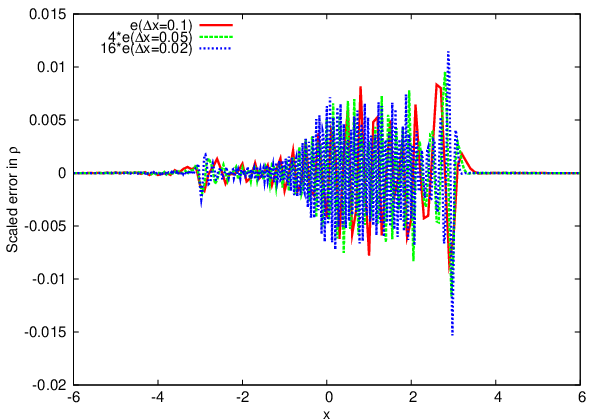
As can be seen the errors are as high frequency as can be allowed given the spatial resolution, i.e. the error varies dramatically from grid point to grid point. Therefore it is impossible to talk about pointwise convergence since the error at a given gridpoint may be positive at one resolution but negative at another. However, the amplitude in the error can still be considered second order convergent. In fact calculating the discrete L2-norm of the error we find that and showing that we have global second order convergence in the L2-norm. The numerical methods used here are formally fourth order accurate, but because the source is we are limited to only second order convergence.
If instead we use the source
| (72) |
with the same values for and as before we obtain the scaled errors shown in Figure 13.

Here the errors are smooth and low frequency and the scaled errors from different resolutions (scaled for fourth order convergence) agree very well, i.e. we have pointwise convergence. For the L2-norms of the errors in this case, we get and , clearly showing the expected reduction in errors by a factor of 16 with a doubling of the resolution.
Appendix B Self-force as boundary integrals in Kerr-Schild coordinates
In this Appendix, we derive the relationship between the (Kerr-Schild) time-component of the self-force on the scalar charge and the energy flux at spatial infinity and across the event horizon. We also derive explicit expressions for these fluxes in Kerr-Schild coordinates.
B.1 How and the energy flux are related for charges in circular orbits
For a scalar charge going in a circular orbit around a Schwarzschild black hole, there exists a direct relationship between the time-component of the self-force on the scalar charge and the energy flux at spatial infinity and across the event horizon.
In the absence of external fields, the motion of a scalar particle is governed by the self-force acting on it,
| (73) |
The energy per unit mass (i.e. specific energy) of a particle along a geodesic with a four-velocity is just , where is the time-translation Killing vector of the Schwarzschild spacetime. The rate of change in this specific energy per unit proper time is , since . In Kerr-Schild coordinates this is just . Evaluating this on a particle moving in a circular orbit, Eq. (73) gives us,
| (74) | ||||
| (75) |
where signifies the location of the particle. The second term in the first equality vanishes for a circular orbit,
| (76) | ||||
| (77) | ||||
| (78) | ||||
| (79) |
where is the Killing vector associated with the helical symmetry, so that the third equality vanishes due to Eq. (20). Thus
| (80) |
The time component of the self-force in Kerr-Schild coordinates is then just the amount of energy lost by the particle per unit proper time.
This energy loss must obviously be related to the scalar energy flux. We shall now derive these relationships and also the explicit expressions for the energy fluxes in Kerr-Schild coordinates.
The scalar field produced by the charge is determined by the field equation,
| (81) |
Multiply both sides by , integrate over (which we take to be the 4-volume bounded by constant Kerr-Schild -surfaces and , the event horizon, and time-like hypersurface ), and is the time-translation Killing vector of Schwarzschild, and simplify the integral over the delta function to obtain
| (82) |
We notice now that the integrand on the left can be expressed as
| (83) | |||||
where is the stress-energy tensor for the scalar field,
| (84) |
We then have
| (85) |
where, specializing to circular orbits, . Here, we have exploited the fact that requires no regularization and thus equals . Since is a Killing vector, , and is symmetric in its indices, we have . Thus,
| (86) |
| (87) |
where is the directional volume element of the boundary . The integrand of the left hand side is essentially the conserved current for the scalar field, .
We recall again that for the case of a scalar charge in a perpetual circular orbit of angular velocity , there exists a helical Killing vector given by
| (88) |
We break up the left hand side of Eq. (87) into the four hypersurface integrals,
| (89) |
is the null generator of the event horizon, and the rest of the hatted quantities are the respective outward unit normal vectors to the other hypersurfaces making up . is an arbitrary parameter on the null generators of the event horizon. From the helical symmetry of the problem it is easy to see that the last two integrals just cancel each other out. This simply means that energy content in each constant- hypersurface is the same. But we can show this explicitly.
Consider the time evolution of the total energy in a -hypersurface,
| (90) |
where we have used the helical symmetry , for any . In other words, time evolution is really just axial rotation.
Thus, for a circular orbit , Eq. (87) becomes
| (91) |
For convenience, we may set the arbitrary parameter on the horizon to be . If we then differentiate both sides with respect to , we finally get
| (92) |
where
| (93) | ||||
| (94) |
These are the general formulas for the energy flux at spatial infinity and the event horizon. In the next section, we write them out explicitly in terms of and its derivatives.
Finally, Eqn. (92) can be written in the form,
| (95) |
where is the specific energy of a particle moving along a geodesic. This is just a statement of the conservation of energy: the energy lost by the charge is also the energy flowing through and .
B.2 Scalar energy flux in Kerr-Schild coordinates
For convenience we write Eqs. (93) and (94) in terms of and its derivatives, in Kerr-Schild coordinates. These formulas are essentially the same except for their unit normals, where one is null and the other spacelike.
We first note that in Kerr-Schild coordinates, the Schwarzschild metric and its inverse are simply
| (96) | ||||
| (97) |
| (98) |
where and .
We begin first with the energy flux through the event horizon. The event horizon is essentially a surface of constant retarded time , where the subscript means that these are Schwarzschild coordinates. In Kerr-Schild coordinates these surfaces of constant are
| (99) |
where is just a constant. Any particular surface in this family can be defined parametrically by the equations,
| (100) | ||||
| (101) | ||||
| (102) | ||||
| (103) |
where is defined implicitly by the relation
| (104) |
With this, the null generator of the surface (which is also normal to it) is
| (105) |
With the stress-energy tensor given by Eq. (84) and using the expressions given in Eqs.(96)-(98), a small amount of algebra yields
| (106) |
where the overdot means a derivative with respect to . At , the energy flux is then simply just
| (107) |
The normal one-form associated with the hypersurface is . The corresponding normalized vector is then
| (108) |
This leads to the following
| (109) |
Thus, the flux through which is just
| (110) |
Taking the limit , this reduces to the more familiar flat spacetime case,
| (111) |
And so, we have for the energy flux at spatial infinity,
| (112) |
One of the internal checks we perform is to verify that Eq. (92) holds by computing the -component of the self-force and the fluxes given in equations (107) and (110).
Appendix C A toy illustration of our method
Partial differential equations with two dramatically different length scales are difficult to solve with numerical analysis. Consider the example of a scalar field of a spherical object at rest, centered at and with a small radius . And, the small object has a scalar charge density , with being constant for and being zero for . The small object is inside a much larger odd-shaped box, and on the surface of the box is the Dirichlet boundary condition for . For simplicity assume that spacetime is flat and, with the object at rest, there is no radiation and the field equation is elliptic. Then
| (113) |
where is the usual three-dimensional flat space gradient operator.
The challenge is to numerically determine the actual field as a function of everywhere inside the box, subject to the field equation (113) and the boundary condition, and then to find the total force on the small object which results from its interaction with .
On the one hand a very fine numerical grid is necessary to resolve in and around the object particularly for obtaining the force acting on the object. On the other hand, a coarse grid would suit the boundary condition while speeding up the numerical computation. If the ratio of length scales is many orders of magnitude, or if the small object is represented by a delta function then adaptive mesh methods are unlikely to be adequate to resolve the small object while using modest resources.
To confront the difficulty of the task, we find it advantageous to introduce the source field , where
| (114) |
The source field is completely determined by local considerations in the neighborhood of the object, and it is chosen carefully to be an elementary solution of
| (115) |
Sometimes we call the singular field to emphasize the behavior outside but near the small source.
The actual scalar field for the problem at hand is approximately near the small object, and the numerical problem may be reformulated in terms of the remainder field
| (116) |
which is then a solution of
| (117) |
where the second equality follows from Eq. (115). The is thus a source free solution of the field equation, and we sometimes call it the regular field because the singular is removed from the actual field in Eq. (116). And if is determined then simply adding it to the analytically known provides .
A drawback to this formulation might be that the boundary condition requires that on the boundary of the box. This is likely to be more difficult to impose than the original boundary condition.
A variation of this approach resurrects the original boundary condition. We introduce a window function that obeys three properties:
- A.
in a neighborhood which includes the entire source , that is all , but the neighborhood might be larger.
- B.
for greater than some value which is not very small.
- C.
has no structure on the small length scale
Then we modify the source field to be . Now the field equation for the regular field becomes
| (118) |
and this defines a source that is zero throughout the small object, is zero at the boundary and shows no variation on the small length scale . So, as long as is smooth enough, the boundary condition for is the natural condition that .
In terms of the original source field , the source for is
| (119) | |||||
where the third equality follows from Eq. (115) and from property A of the window function.
In the formulation based upon Eq. (118), the small length scale has been completely removed from the problem. The field ought to be relatively easy to evaluate, and then the actual field is trivial to determine.
This formulation has the bonus that it simplifies the calculation of the force on the object from the field. The net force is an integral over the volume of the object,
| (120) |
In the original formulation of Eq. (113), the actual field in the integral would be dominated by which changes dramatically over the length scale of the object, and could be lost easily in the noise of the computation. The fact that and are spherically symmetric implies that
| (121) |
Then the substitution in the integral of Eq. (120) leads to the conclusion that
| (122) |
Thus the force acting on the object depends only upon the field .
In addition, the field does not change significantly over a small length scale, so if the object is extremely small or even a delta function source then an accurate approximation to the force is
| (123) |
This redefinition of the problem at hand is broad enough to encompass a suggestion by Barack and Golbourn [30] to use a window function that is a step function of unity in an inner region containing the small object and zero everywhere outside the region. An implementation of this idea involves solving for outside the region, with the original boundary condition on the box, and solving for within the inner region, with the additional boundary conditions that the value and the normal derivative of match those of on the boundary of the inner region.
If the source is replaced by a delta function then if and is with all derivatives of vanishing at , then for all and the source in Eq. (119) is . However, if the th derivative of is not zero at , then the source is only . Or, if for some reason the exact expression for is not known, and only an expansion is available, then again the source may be of only limited differentiability.
In applications of this approach to problems in curved spacetime, the singular field is rarely known exactly. This limits the differentiability of the source of Eq. (119) which, in turn, limits the differentiability of the remainder at the particle.
References
- [1] C. Hopman and T. Alexander, The orbital statistics of stellar inspiral and relaxation near a massive black hole: characterizing graviational wave sources, Astrophys. J. 629, 362 (2005), eprint astro-ph/0503672.
- [2] P. Amaro-Seoane, J. R. Gair, M. Freitag, M. C. Miller, I. Mandel, C. J. Cutler, and S. Babak, Intermediate and extreme mass-ratio inspirals – astrophysis, science applications and detection using LISA, Class. Quantum Grav. 24, R113 (2007), eprint astro-ph/0703495.
- [3] T. Regge and J. A. Wheeler, Stability of a Schwarzschild singularity, Phys. Rev. 108, 1063 (1957).
- [4] F. J. Zerilli, Gravitational field of a particle falling in a Schwarzschild geometry analyzed in tensor harmonics, Phys. Rev. D 2, 2141 (1970).
- [5] S. A. Teukolsky, Perturbations of a rotating black hole. I. fundamental equations for gravitational, electromagnetic and neutrino-field perturbations, Astrophys. J. 185, 635 (1973).
- [6] S. Detweiler, Perspective on gravitational self-force analyses, Class. Quantum Grav. 15, S681 (2005), eprint gr-qc/0501004.
- [7] Y. Mino, M. Sasaki, and T. Tanaka, Gravitational radiation reaction to a particle motion, Phys. Rev. D 55, 3457 (1997), eprint gr-qc/9606018.
- [8] T. C. Quinn and R. M. Wald, Axiomatic approach to electromagnetic and gravitational radiation reaction of particles in curved spacetime, Phys. Rev. D 56, 3381 (1997), eprint gr-qc/9610053.
- [9] E. Poisson, The motion of point particles in curved spacetime, Living Rev. Relativity 7, 6 (2004), http://www.livingreviews.org/lrr-2004-6.
- [10] W. G. Anderson and A. G. Wiseman, A matched expansion approach to practical self-force calculations, Class. Quantum Grav. 22, S783 (2005), eprint gr-qc/0903.0395.
- [11] M. Casals, S. Dolan, A. C. Ottewill, and B. Wardell, Self-force calculations with matched expansions and quasinormal mode sums, Phys. Rev. D 79, 124043 (2009), eprint gr-qc/0903.0395.
- [12] L. Barack, Gravitational self-force by mode sum regularization, Phys. Rev. D 64, 084021 (2001), eprint gr-qc/0105040.
- [13] L. Barack, Y. Mino, H. Nakano, A. Ori, and M. Sasaki, Calculating the gravitational self force in the Schwarzschild spacetime, Phys. Rev. Lett. 88, 091101 (2002), eprint gr-qc/0111001.
- [14] L. Barack and A. Ori, Regularization parameters for the self force in Schwarzschild spacetime: I. scalar case, Phys. Rev. D 66, 084022 (2002), eprint gr-qc/0204093.
- [15] S. Detweiler and B. F. Whiting, Self-force via a Green’s function decomposition, Phys. Rev. D 67, 024025 (2003), eprint gr-qc/0202086.
- [16] S. Detweiler, E. Messaritaki, and B. F. Whiting, Self-force of a scalar field for circular orbits about a Schwarzschild black hole, Phys. Rev. D 67, 104016 (2003), eprint gr-qc/0205079.
- [17] W. Hikida, H. Nakano, and M. Sasaki, A new analytical method for self-force regularization I. charged scalar particles in Schwarzschild spacetime, Prog. Theor. Phys. 111, 821 (2004a), eprint gr-qc/0308068.
- [18] W. Hikida, H. Nakano, and M. Sasaki, A new analytical method for self-force regularization II. testing the efficiency for circular orbits, Prog. Theor. Phys. (2004b), eprint gr-qc/0410115.
- [19] W. Hikida, H. Nakano, and M. Sasaki, Self-force regularization in the Schwarzschild spacetime, Class. Quantum Grav. (2004c), eprint gr-qc/0411150.
- [20] L. M. Diaz-Rivera, E. Messaritaki, B. Whiting, and S. Detweiler, Scalar field self-force effects on orbits about a Schwarzschild black hole, Phys. Rev. D 70, 124018 (2004), eprint gr-qc/0410011.
- [21] R. Haas and E. Poisson, Mode-sum regularization of the scalar self-force: Formulation in terms of a tetrad decomposition of the singular field, Phys. Rev. D 74, 044009 (2006), eprint gr-qc/0605077.
- [22] R. Haas, Scalar self-force on eccentric geodesics in schwarzschild spacetime: A time-domain computation, Phys. Rev. D 75, 124011 (2007), eprint gr-qc/0704.0797.
- [23] I. Vega and S. Detweiler, Regularization of fields for self-force problems in curved spacetime: Foundations and a time-domain application, Phys. Rev. D 77, 084008 (2008), eprint gr-qc/0712.4405.
- [24] S. Detweiler, Consequence of the gravitational self-force for circular orbits of the Schwarzschild geometry, Phys. Rev. D 77, 124026 (2008), eprint gr-qc/0804.3529.
- [25] L. M. Burko, Self force on particle in orbit around a black hole, Phys. Rev. Lett. 84, 4529 (2000), eprint gr-qc/0003074.
- [26] R. Haas, Time domain calculation of the electromagnetic self-force on eccentric geodesics in Schwarzschild spacetime, in preparation.
- [27] L. Barack and N. Sago, Gravitational self force on a particle in circular orbit around a schwarzschild black hole, Phys. Rev. D 75, 064021 (2007), eprint gr-qc/0701069.
- [28] N. Sago, L. Barack, and S. Detweiler, Two approaches for the gravitational self force in black hole spacetime: Comparison of numerical results, Phys. Rev. D78, 124024 (2008), eprint 0810.2530.
- [29] N. Warburton and L. Barack, Self-force on a scalar charge in Kerr spacetime: circular equatorial orbits, in preparation.
- [30] L. Barack and D. A. Golbourn, Scalar-field perturbations from a particle orbiting a black hole using numerical evolution in 2+1 dimensions, Phys. Rev. D 76, 044020 (2007), eprint gr-qc/0705.3620.
- [31] L. Barack, D. A. Golbourn, and N. Sago, -mode regularization scheme for the self-force in Kerr spacetime, Phys. Rev. D 76, 124036 (2007), eprint gr-qc/0709.4588.
- [32] P. Cañizares and C. F. Sopuerta, Efficient pseudospectral method for the computation of the self-force on a charged particle: Circular geodesics around a Schwarzschild black hole, Phys. Rev. D 79, 084020 (2009), eprint gr-qc/0903.0505.
- [33] E. Schnetter, P. Diener, N. Dorband, and M. Tiglio, A multi-block infrastructure for three-dimensional time-dependent numerical relativity, Class. Quantum Grav. 23, S553 (2006), eprint gr-qc/0602104.
- [34] W. Tichy, Black hole evolution with the bssn system by pseudo-spectral methods, Phys. Rev. D 74, 0840005 (2006), eprint gr-qc/0609087.
- [35] A. S. Eddington, A comparison of Whitehead’s and Einstein’s formulae, Nature 113, 192 (1924).
- [36] J. W. York, Kinematics and dynamics of General Relativity, in Sources of Gravitational Radiation, edited by L. Smarr (Cambridge University Press, Cambridge, 1979), pp. 83–126.
- [37] B. Dewitt and R. Brehme, Radiation damping in a gravitational field, Annals of Physics 9, 220 (1960).
- [38] K. S. Thorne and J. B. Hartle, Laws of motion and precession for black holes and other bodies, Phys. Rev. D 31, 1815 (1985).
- [39] X.-H. Zhang, Multipole Expansions of the General-Relativistic Gravitational Field of the External Universe, Phys. Rev. D 34, 991 (1986).
- [40] S. Detweiler, Radiation reaction and the self-force for a point mass in General Relativity, Phys. Rev. Lett. 86, 1931 (2001), eprint gr-qc/0011039.
- [41] N. Yunes, W. Tichy, B. J. Owen, and B. Bruegmann, Binary black hole initial data from matched asymptotic expansions, Phys. Rev. D 74, 104011 (2006), eprint gr-qc/0503011.
- [42] D. Finkelstein, Past-future assymetry of the gravitational field of a point particle, Phy. Rev. 110, 965 (1958).
- [43] P. Diener, E. N. Dorband, E. Schnetter, and M. Tiglio, Optimized high-order derivative and dissipation operators satisfying summation by parts, and applications in three-dimensional multi-block evolutions, J. Sci. Comput. 32, 109 (2007), eprint gr-qc/0512001.
- [44] E. N. Dorband, E. Berti, P. Diener, E. Schnetter, and M. Tiglio, A numerical study of the quasinormal mode excitation of Kerr black holes, Phys. Rev. D 74, 084028 (2006), eprint gr-qc/0608091.
- [45] W. Tichy, Long term black hole evolution with the bssn system by pseudo-spectral methods, Long term black hole evolution with the BSSN system by pseudo-spectral methods, in preparation.
- [46] W. Tichy, A new numerical method to construct binary neutron star initial data (2009), eprint gr-gc/0908.0620.
- [47] M. A. Scheel et al., 3D simulations of linearized scalar fields in Kerr spacetime, Phys. Rev. D69, 104006 (2004), eprint gr-qc/0305027.
- [48] R. Lopez-Aleman, G. Khanna, and J. Pullin, Perturbative evolution of particle orbits around Kerr black holes: time domain calculation, Classical and Quantum Gravity 20, 3259 (2003), eprint gr-qc/0303054.
- [49] L. M. Burko and G. Khanna, Accurate time-domain gravitational waveforms for extreme-mass-ratio binaries, Europhysics Letters 78, 60005 (2007), eprint gr-qc/0609002.
- [50] P. A. Sundararajan, G. Khanna, and S. A. Hughes, Towards adiabatic waveforms for inspiral into Kerr black holes: I. a new model of the source for the time domain perturbation equation, Phys. Rev. D 76, 104005 (2007), eprint gr-qc/0703028.
- [51] S. R. Lau, Rapid evaluation of radiation boundary kernels for time- domain wave propagation on black holes: Implementation and numerical tests, Class. Quant. Grav. 21, 4147 (2004).
- [52] S. E. Field, J. S. Hesthaven, and S. R. Lau, Discontinuous Galerkin method for computing gravitational waveforms from extreme mass ratio binaries (2009), eprint gr-qc/0902.1287.