The Phase Structure of Supersymmetric Gauge Theories with an Adjoint
David Poland
Jefferson Physical Laboratory, Harvard University,
Cambridge, Massachusetts 02138, USA
August 24, 2026
We study the phase structure of supersymmetric gauge theories with fundamentals, an adjoint, and vanishing superpotential. Using a-maximization, we derive analytic expressions for the values of below which the first several gauge-invariant operators in the chiral ring violate the unitarity bound and become free fields. In doing so we are able to explicitly check previous conjectures about the behavior of this theory made by Luty, Schmaltz, and Terning. We then compare this to an analysis of the first two ’deconfined’ dual descriptions based on the gauge groups and , finding precise agreement. In particular, we find no evidence for non-obvious accidental symmetries or the appearance of a mixed phase in which one of the dual gauge groups becomes free.
1 Introduction
It is of great interest to understand the low-energy behavior of asymptotically free gauge theories. Analyzing such theories in the strong-coupling regime is generally quite difficult, but can become tractable with a sufficient amount of symmetry. Strongly-coupled gauge theories with supersymmetry are particularly interesting in that they are both amenable to analysis and potentially relevant for phenomenology. Possible applications include dynamical supersymmetry breaking [1, 2, 3], conformal sequestering [4, 5], dynamical solutions to the -problem [6, 7, 8], dynamical explanations of the flavor hierarchies [9, 10, 11], dynamical solutions to the doublet-triplet splitting problem [12, 13, 14], and so on.
When analyzing a supersymmetric gauge theory, a first-order question is to determine what kind of phase the theory flows to at low energies. Possibilities include that the theory is infrared (IR) free, the theory flows to an interacting conformal (non-Abelian Coulomb) phase, the theory has a ’dual’ description that is IR free, the theory confines, the theory dynamically generates a superpotential that breaks the gauge group, or that the theory enters a pure Abelian Coulomb phase (see [15, 16] for reviews). In addition, it is possible that the theory enters a ’mixed phase’ consisting of decoupled sectors that are in some combination of the above phases. This can occur, e.g., when the theory is in an interacting conformal regime but some set of operators have become free fields and decoupled from the CFT. More exotically, the theory could have a dual description containing a product gauge group in which one gauge group is interacting and one gauge group is IR free. This was argued to occur, e.g., in gauge theories with an anti-symmetric tensor [17, 18].
An important tool for studying theories in a conformal regime, a-maximization, was introduced by Intriligator and Wecht in [19], and further developed in [20, 21, 22]. The idea is that the correct superconformal symmetry can be determined by maximizing
| (1.1) |
over all possible trial R-symmetries , where is any initial R-symmetry and are the IR flavor symmetries. This is an extremely powerful technique provided that one understands the IR flavor symmetries. Unfortunately, one cannot always identify the IR flavor symmetries as a subset of the UV flavor symmetries – accidental symmetries can arise (see, e.g., [23] for a number of interesting examples).
How can one gain evidence for accidental symmetries? One way is to check whether there are any gauge-invariant operators in the chiral ring of the theory that violate the unitarity bound, given by for scalar operators [24]. If this bound appears to be violated, then one plausible interpretation is that is becoming a free field with . In this case there is an accidental symmetry associated with rotations of , and one must include this symmetry when maximizing . In practice, this requires one to instead maximize [25, 20]
| (1.2) |
However, not all accidental symmetries manifest themselves through apparent violations of unitarity. This happens for example in gauge theories with flavors of vector-like quarks in the range [26]. Since the anomaly-free symmetry is , the mesons appear to violate the unitarity bound in this range and presumably become free fields. However, this is only part of the story, as it is also believed that the entire dual gauge group and the corresponding dual quarks are also becoming free fields, yielding many more accidental symmetries. This is not obvious in the original ’electric’ description of the theory, but becomes apparent when the dual ’magnetic’ description is analyzed. When studying similar theories, it is clearly of great interest to have dual descriptions available that can be studied, as they may contain evidence for the emergence of non-obvious accidental IR symmetries.
In the present work we will use a-maximization to study supersymmetric gauge theory with fundamentals and an adjoint . While the theory with superpotential is fairly well understood [27], the theory with vanishing superpotential has not been as easy to analyze. An attempt to study this theory using ’deconfinement’ [28] was made in [29], where it was proposed that the theory has a sequence of dual descriptions, the first of which is based on an gauge theory. However, because the symmetry of the theory was unknown it was not possible to determine which operators, if any, gave apparent violations of the unitarity bound as one varies and . Furthermore, it was not possible to explicitly check the dual descriptions for evidence of additional accidental symmetries, as would occur if either of the dual gauge groups were becoming free. As we will see, such an analysis is now possible using a-maximization, and we will here present an attempt to map out the phase structure of the theory. Similar studies of other theories have appeared in [20, 30, 18, 31, 32, 33].
This paper is organized as follows. In section 2 we use a-maximization to study gauge theory with an adjoint. In sections 3 and 4 we perform a similar analysis of the first two dual descriptions of the theory, comparing the results and looking for evidence of accidental IR symmetries. We give concluding remarks in section 5.
2 Gauge Theory with an Adjoint
We are interested in studying supersymmetric gauge theory11 1 Our conventions are such that . with fundamentals and an adjoint . The field content and anomaly-free symmetries are given in Table 1.
| 1 | ||||
| 1 | -1 | 0 |
In particular, we are here interested in the theory with vanishing superpotential. It is believed that this theory is in an interacting conformal regime for all .
The chiral ring of this theory contains the gauge-invariant operators
| (2.1) |
As mentioned in the introduction, this theory was previously studied using ’deconfinement’ in [29], where it was conjectured that the operators sequentially become free fields as is decreased from the asymptotic freedom limit of while the remain interacting. It was also noted in [31] that the large limit of this theory will yield the same R-charges as gauge theory with flavors and an adjoint, which was studied in [20]. Here we will attempt to map out the phase space allowing for smaller and , comparing our results to the conjectures of [29]. In particular, we will find that both the operators and sequentially become free fields as is decreased, with the precise order depending on the value of . This realizes the behavior that was described as scenario C in [29], and thus we will prove that the conjectured behavior (scenario A) is incorrect.
In order to determine the symmetry of the theory, we should maximize subject to the constraint that the mixed anomalies vanish. Recall that an adjoint of is a two-index symmetric tensor with index and dimension . Anomaly cancellation then requires
| (2.2) |
or equivalently
| (2.3) |
In order to determine the R-symmetry, we should then maximize
| (2.4) | |||||
The correct solution to is then given by
| (2.5) |
where the positive root of the quadratic equation is picked out by requiring that this be a maximum.
Now we can ask the question of which gauge-invariant operator is the first to violate the unitarity bound as we lower from . It is straightforward to solve the condition for . This gives the condition that the operator is at or below the unitarity bound when
| (2.6) |
On the other hand, we should check that does not hit the unitarity bound first. The condition is equivalent to
| (2.7) |
which is less than for positive . Thus, within the entire region
| (2.8) |
When is below this threshold we assume that becomes a free field, and we should modify the a-maximization procedure according to the prescription given in [20]. Thus, we should now maximize the function
| (2.9) |
Again solving yields the the solution
| (2.10) | |||||
where the positive root is again picked out by requiring that this be a maximum.
Now that we know the R-symmetry in this region, we can determine which operator is next to hit the unitarity bound. It is straightforward to show that the condition that is equivalent to
| (2.11) |
This should be compared to the condition for , which occurs when
| (2.12) |
It is then easily verified that in the entire region
| (2.13) |
Below this threshold we can repeat the procedure, treating as a free field, and maximize
| (2.14) |
Solving then yields the maximum
| (2.15) | |||||
Now we find that when
| (2.16) |
and when
| (2.17) |
The structure this time is somewhat more complicated. If then gives the stronger bound, and if then gives the stronger bound. However, over a wide range of the difference between these functions is , and and hit the unitarity bound at approximately the same values of . In any case, since we are here primarily interested in mapping out the phase structure for smaller values of and , we will first consider the case that decouples at the larger value of .
Treating as a free field below the threshold in Eq. (2.16), we should now maximize
| (2.18) |
which gives
| (2.19) | |||||
We can then determine that when
| (2.20) |
and when
| (2.21) |
Comparing these functions, we find that decouples at the larger value of for all . On the other hand, if , then the bound is only potentially applicable for . Thus, is the next operator to decouple except in the special case of , and this decoupling occurs when is below the threshold given in Eq. (2.21).
As an immediate check on the results obtained so far, we can expand Eqs. (2.17) and (2.21) in the limit of large . Since the effect of decoupling can be neglected in this limit, they should agree up to terms of . In addition, as was noted in [31], the resulting bound on below which becomes free should reproduce the results of [20]. We find these checks to be successful. In the large limit we obtain that becomes a free field when
| (2.22) |
which does indeed agree with [20] at leading order.
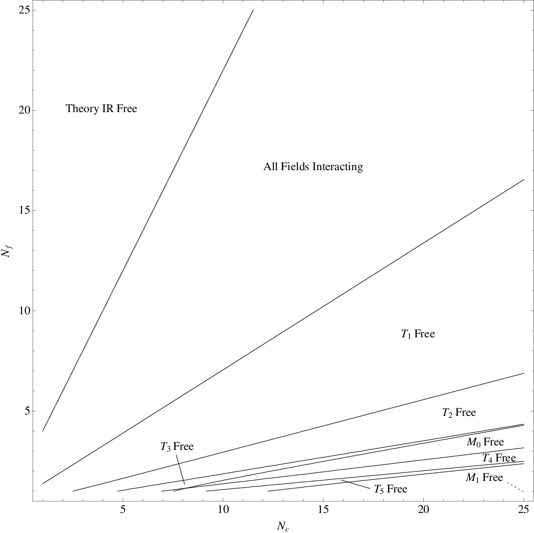
Of course, one can continue this procedure indefinitely. On the other hand, if one is primarily interested in smaller values of and , the region of interest is quickly filled in. In Figure 1 we show an approximate phase space diagram for the theory including the next several decoupling thresholds (though we will suppress the analytic expressions). Since the case of is somewhat more complicated, we give its structure separately in Table 2.
| 1 | 2 | 3 | 4 | 5 | 6 | 7 | 8 | 9 | 10 | 11 | 12 | 13 | 14 | 15 | 16 | 17 | 18 | 19 | |
|---|---|---|---|---|---|---|---|---|---|---|---|---|---|---|---|---|---|---|---|
3 First Deconfined Dual Description
One potential danger with the analysis presented in the previous section is that it may be overlooking non-obvious accidental symmetries that may emerge due to the strong dynamics. This happens, e.g., in gauge theories with flavors in the range . In that situation, there are accidental symmetries associated with the dual quarks and gauge bosons becoming free fields in the IR. This is manifest when the theory is studied in the dual magnetic description, but completely non-obvious in the electric description. Thus, it is great interest to study dual descriptions of the present scenario in order to look for evidence for a similar scenario.
Fortunately, this theory in fact has a sequence of dual descriptions that can be studied [29]. The dualities are obtained via ’deconfinement’, and involve promoting the adjoint to a composite state in a strongly-coupled theory. The first dual description is then obtained by taking and dualizing the original gauge group using the known duality for gauge groups with only fundamentals [34]. The end result of this procedure is given in Table 3. In addition, the theory has a superpotential
| (3.1) |
and the mapping between the gauge-invariant operators in the original and dual description is given by
| (3.2) |
| 1 | 0 | ||||
| 1 | 1 | 2 | |||
| 1 | 1 | ||||
| 1 | 1 | 0 | |||
| 1 | 1 | ||||
| 1 | 1 | 5 | |||
| 1 | 1 | -3 | |||
| 1 | 1 | 1 | 6 |
Now, if one just considers the one-loop beta function it naïvely seems that the gauge group is IR free for . However, this is misleading because, e.g., the strong gauge group gives a large anomalous dimension to the bi-fundamental , which in turn gives an correction to the full beta function. This is an example of a larger class of RG flows in product group theories (see [35, 31] for many examples) in which an otherwise IR free coupling can be driven to be interacting because of the other gauge group.
Thus, we will proceed by assuming that the full theory is interacting, again using a-maximization to decide if any fields become free. In particular, we should require that the symmetry is anomaly free with respect to both gauge groups, i.e. that both the and anomalies vanish. Furthermore, we will start by assuming that the full superpotential in Eq. (3.1) is marginal. Notice that anomaly cancellation and the superpotential together give 7 constraints on 8 unknown charges, causing to again be a function of a single variable as in the previous section.
More concretely, the constraints are
| (3.3) |
These linear equations can be solved to express all of the R-charges in terms of , yielding
| (3.4) |
Equivalently, we could have obtained these expressions simply by considering the linear combination , where and are the and charges of each field as given in Table 3.
In order to determine we should then maximize the function
| (3.5) | |||||
Remarkably, the solution to corresponding to the maximum is
| (3.6) |
which coincides exactly with Eq. (2.5)! Moreover, the function Eq. (3.5) is precisely equal to Eq. (2.4). Of course, one may view this as a consequence of the fact that the ’t Hooft anomalies of the dual description were designed to match those of the original theory. Nevertheless, we can perhaps view this agreement as a non-trivial check of the dynamical assumptions that both gauge groups are interacting and that the full superpotential Eq. (3.1) is marginal, at least for the values of that do not lead to violations of the unitarity bound.
Since the function is the same as before, the operators hit the unitarity bound at the same thresholds as before. In particular, becomes a free field for . Below this threshold we can maximize
| (3.7) |
This then yields the same result as Eq. (2.10). The precise agreement between the dual description and the original description then continues, with becoming free at the threshold given in Eq. (2.11) and becoming free at the threshold given in Eq. (2.16) (for ).
Now, one might worry that the situation changes when violates the unitarity bound and becomes a free field. This occurs either below the threshold given in Eq. (2.17) or Eq. (2.21), depending on the value of (or at for ). When this happens, the superpotential term must be flowing to zero, since this is ’s only interaction. In addition, for just above this threshold, we know that due to the superpotential interaction. A possible interpretation of this is that the gauge group is becoming free. Under this interpretation, the coupling is flowing to zero because unitarity is now enforcing the condition that . Note that in this case one would still expect the gauge group to be strongly coupled. If this interpretation is correct, this would be similar to the mixed phase argued to exist in gauge theories with an anti-symmetric tensor [17, 18]. In addition, there would be accidental symmetries emerging that would invalidate the a-maximization analysis performed in the electric description of the theory.
However, we will now argue that this scenario cannot be correct. To do this we will consider the sign of the -function in the hypothetical mixed phase. As mentioned above, since we are assuming that is becoming free we must now have and by unitarity, and thus we know that the couplings and must also become irrelevant. The interacting sector of the theory then simply consists of the fields , with superpotential
| (3.8) |
Now, in order for this scenario to be plausible the -function should be positive so that the fixed point is IR attractive. This then requires that , or more explicitly
| (3.9) |
Because the superpotential and anomaly cancellation constraints lead to the same parametrization of the R-charges (for the interacting fields) as was given in Eq. (3.4), this condition is equivalent to
| (3.10) |
Since we expect the theory to have so as to avoid an infinite number of free operators, this bound will never be satisfied. For example, in the limit of large we obtain
| (3.11) |
and the full calculation gives qualitatively similar results. Note that it can be also verified that no subset of the couplings in Eq. 3.8 leads to an IR stable fixed point. Thus, we conclude that is not an IR attractive fixed point in the hypothetical mixed phase, and that both gauge groups must remain interacting even after becomes free.22 2 It is also interesting to note that entering the hypothetical mixed phase would have required violating the (stronger) conjecture of Ref. [36] that operators with cannot become free fields, since in the interacting scenario.
4 Second Deconfined Dual Description
Now we will consider the second dual description constructed in [29], which can be obtained by treating the anti-symmetric tensor as a meson of a confining gauge theory, and then dualizing the gauge group using the known duality for gauge theories with fundamentals [26, 37]. The field content (after integrating out massive fields) is given in Table 4. In addition, the theory has the superpotential
| (4.1) | |||||
and the gauge-invariant operators of the electric theory match onto the operators
| (4.2) |
| 1 | 1 | 1 | 2 | |||
| 1 | 1 | 0 | ||||
| 1 | 1 | 1 | 2 | |||
| 1 | 1 | 1 | ||||
| 1 | 1 | 1 | 0 | |||
| 1 | 1 | 0 | ||||
| 1 | 1 | 1 | 2 | |||
| 1 | 1 | 1 | ||||
| 1 | 1 | 1 | 1 | 0 | ||
| 1 | 1 | 1 | 1 | |||
| 1 | 1 | 1 | 1 | |||
| 1 | 1 | 1 | 5 | |||
| 1 | 1 | 1 | -3 | |||
| 1 | 1 | 1 | 1 | 6 | ||
| 1 | 1 | 1 | 1 |
We can again begin by assuming that each of the gauge groups are interacting and that the entire superpotential in Eq. 4.1 is marginal. This gives 3 constraints from anomaly cancellation and 11 constraints from the superpotential on 15 unknown R-charges, causing to again be a function of a single variable (as expected). The R-charges of each field are then easily obtained in terms of by considering the linear combination
| (4.3) |
where and are the and charges given in Table 4. Alternatively, this parametrization could be obtained by using the 14 constraints to solve for the 15 unknown R-charges in terms , as we did in the previous section.
It is then straightforward to verify that the function
| (4.4) | |||||
is exactly equal to the functions given in Eqs. (2.4) and (3.5). In particular, maximizing it gives rise to the same symmetry as was found in the previous sections. Furthermore, the operators become free fields at the same thresholds as before as we lower from .33 3 It is perhaps worrisome that the gauge-invariant operator appears to badly violate the unitarity bound, since it has . However, if the duality is to be believed, non-perturbative effects in this description should cause this operator to be zero in the chiral ring in order to avoid a contradiction.
When the operator hits the unitarity bound we assume that the coupling is simply flowing to zero so that can become a free field. Note that this is unlikely be the result of the gauge coupling flowing to zero because this would also force to be a free field and one would expect that close to this threshold, which is not the case. Furthermore, the gauge group going free would not cause this operator to become irrelevant.
Thus we first consider the possibility that, similar to the hypothetical mixed phase considered in the previous section, the gauge group is becoming free when hits the unitarity bound. If this is the case, unitarity requires that and forces the couplings and to become irrelevant. The interacting superpotential of the mixed phase then becomes
| (4.5) | |||||
along with the free fields and potentially free operators .
The superpotential combined with anomaly cancellation then give 10 constraints on 11 unknown R-charges, with the same parametrization for the R-charges of the interacting fields as in Eq. 4.3. However, again we can rewrite the condition that as
| (4.6) |
and this scenario is disfavored for the same reason as in first dual. It is straightforward to additionally verify that no subset of the couplings in Eq. 4.5 lead to an IR attractive fixed point.
Next we would like to investigate the possibility that when becomes a free field the gauge coupling is flowing to zero. Note that in this case unitarity is forcing the coupling to become irrelevant. To see if this is plausible we can again attempt to determine the symmetry of the hypothetical mixed phase and check the sign of the -function.
If it is correct that the gauge coupling flows to zero, unitarity also requires that in addition to . These conditions imply that the couplings , , and should become irrelevant, and thus it is reasonable to assume that the interacting superpotential becomes
| (4.7) |
along with the free fields and potentially free operators . Since we now have 8 constraints and 10 unknown R-charges, will be a function of 2 variables and is best maximized numerically. Doing this, however, we find that the function has no stable maximum and thus the fixed point does not exist.
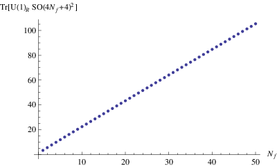
If we turn off one additional coupling, we find that the only IR stable choice is to assume that is flowing to zero – i.e., only this operator has in the hypothetical CFT in which it is absent from the superpotential. However, in this case one can then check that for all and , and hence the assumption that is not correct. To illustrate this, in Figure 2 we plot as a function of in the limit of large . We have also checked that no subset of these couplings leads to an IR stable fixed point. We thus do not find any evidence for a mixed phase in this description of the theory.
5 Conclusions
In this work we have attempted to map out the phase structure of supersymmetric gauge theories with fundamentals, an adjoint, and vanishing superpotential. The IR behavior of this theory has an incredibly rich structure and has previously been difficult to analyze. Using a-maximization, however, we have been able to check the conjectures of [29] as well as look for evidence that the theory enters a mixed phase below some value of . We have not found any such evidence in the simplest known dual descriptions of the theory. It is thus tempting to believe (though far from proven) that the original electric description of the theory is a good description for all and .
A straightforward extension of the present work would be to construct the deconfined dual descriptions of the version of this theory and perform a similar analysis. It would also be quite interesting to find dual descriptions of these theories in which the operators appear as elementary fields so that one could better understand the way in which they decouple from the theory. More generally, it would be interesting to find new examples of theories that possess mixed phases (as in [18]) so that one could better understand and classify the situations under which they can occur. These possible directions are left to future work.
Acknowledgements
We thank Jonathan Heckman, Ken Intriligator, John Mason, David Morrissey, and David Simmons-Duffin for helpful discussions and inspiration. This work is supported in part by the Harvard Center for the Fundamental Laws of Nature and by NSF grant PHY-0556111.
References
- [1] E. Witten, Nucl. Phys. B 188, 513 (1981).
- [2] I. Affleck, M. Dine and N. Seiberg, Phys. Rev. Lett. 51, 1026 (1983); I. Affleck, M. Dine and N. Seiberg, Nucl. Phys. B 241, 493 (1984); I. Affleck, M. Dine and N. Seiberg, Nucl. Phys. B 256, 557 (1985).
- [3]
For reviews, see:
E. Poppitz and S. P. Trivedi, Ann. Rev. Nucl. Part. Sci. 48, 307 (1998) [arXiv:hep-th/9803107]; Y. Shadmi and Y. Shirman, Rev. Mod. Phys. 72, 25 (2000) [arXiv:hep-th/9907225]; K. A. Intriligator and N. Seiberg, Class. Quant. Grav. 24, S741 (2007) [arXiv:hep-ph/0702069]. - [4] M. A. Luty and R. Sundrum, Phys. Rev. D 65, 066004 (2002) [arXiv:hep-th/0105137]; Phys. Rev. D 67, 045007 (2003) [arXiv:hep-th/0111231].
- [5] M. Dine, P. J. Fox, E. Gorbatov, Y. Shadmi, Y. Shirman and S. D. Thomas, Phys. Rev. D 70, 045023 (2004) [arXiv:hep-ph/0405159]; R. Sundrum, Phys. Rev. D 71, 085003 (2005) [arXiv:hep-th/0406012]; M. Ibe, K. I. Izawa, Y. Nakayama, Y. Shinbara and T. Yanagida, Phys. Rev. D 73, 015004 (2006) [arXiv:hep-ph/0506023]; Phys. Rev. D 73, 035012 (2006) [arXiv:hep-ph/0509229]; M. Schmaltz and R. Sundrum, JHEP 0611, 011 (2006) [arXiv:hep-th/0608051]; S. Kachru, L. McAllister and R. Sundrum, [arXiv:hep-th/0703105].
- [6] T. S. Roy and M. Schmaltz, Phys. Rev. D 77, 095008 (2008) [arXiv:0708.3593 [hep-ph]].
- [7] H. Murayama, Y. Nomura and D. Poland, Phys. Rev. D 77, 015005 (2008) [arXiv:0709.0775 [hep-ph]].
- [8] G. Perez, T. S. Roy and M. Schmaltz, [arXiv:0811.3206 [hep-ph]]; H. D. Kim and J. H. Kim, [arXiv:0903.0025 [hep-ph]]; N. J. Craig and D. Green, [arXiv:0905.4088 [hep-ph]].
- [9] A. E. Nelson and M. J. Strassler, JHEP 0009, 030 (2000) [arXiv:hep-ph/0006251]; JHEP 0207, 021 (2002) [arXiv:hep-ph/0104051].
- [10] T. Kobayashi, H. Nakano and H. Terao, Phys. Rev. D 65, 015006 (2002) [arXiv:hep-ph/0107030]; T. Kobayashi, H. Nakano, T. Noguchi and H. Terao, Phys. Rev. D 66, 095011 (2002) [arXiv:hep-ph/0202023].
- [11] D. Poland and D. Simmons-Duffin, [arXiv:0910.4585 [hep-ph]].
- [12] T. Yanagida, Phys. Lett. B 344, 211 (1995) [arXiv:hep-ph/9409329]; T. Hotta, K. I. Izawa and T. Yanagida, Phys. Rev. D 53, 3913 (1996) [arXiv:hep-ph/9509201]; J. Hisano and T. Yanagida, Mod. Phys. Lett. A 10, 3097 (1995) [arXiv:hep-ph/9510277]; T. Hotta, K. I. Izawa and T. Yanagida, Phys. Lett. B 409, 245 (1997) [arXiv:hep-ph/9511431]; T. Hotta, K. I. Izawa and T. Yanagida, Prog. Theor. Phys. 95, 949 (1996) [arXiv:hep-ph/9601320].
- [13] T. Hotta, K. I. Izawa and T. Yanagida, Phys. Rev. D 54, 6970 (1996) [arXiv:hep-ph/9602439]; K. I. Izawa and T. Yanagida, Prog. Theor. Phys. 97, 913 (1997) [arXiv:hep-ph/9703350]; K. I. Izawa and T. Yanagida, Prog. Theor. Phys. 99, 423 (1998) [arXiv:hep-ph/9710218].
- [14] H. C. Cheng, Phys. Lett. B 410, 45 (1997) [arXiv:hep-ph/9702214]; M. Graesser, Phys. Rev. D 59, 035007 (1999) [arXiv:hep-ph/9805417]; R. Kitano and G. D. Kribs, JHEP 0503, 033 (2005) [arXiv:hep-ph/0501047]; Y. Nomura, D. Poland and B. Tweedie, [arXiv:hep-ph/0605014]; R. Kitano, Phys. Rev. D 74, 115002 (2006) [arXiv:hep-ph/0606129].
- [15] K. A. Intriligator and N. Seiberg, Nucl. Phys. Proc. Suppl. 45BC, 1 (1996) [arXiv:hep-th/9509066].
- [16] J. Terning, [arXiv:hep-th/0306119].
- [17] J. Terning, Phys. Lett. B 422, 149 (1998) [arXiv:hep-th/9712167].
- [18] C. Csaki, P. Meade and J. Terning, JHEP 0404, 040 (2004) [arXiv:hep-th/0403062].
- [19] K. A. Intriligator and B. Wecht, Nucl. Phys. B 667, 183 (2003) [arXiv:hep-th/0304128].
- [20] D. Kutasov, A. Parnachev and D. A. Sahakyan, JHEP 0311, 013 (2003) [arXiv:hep-th/0308071].
- [21] D. Kutasov, [arXiv:hep-th/0312098].
- [22] E. Barnes, K. A. Intriligator, B. Wecht and J. Wright, Nucl. Phys. B 702, 131 (2004) [arXiv:hep-th/0408156].
- [23] R. G. Leigh and M. J. Strassler, Nucl. Phys. B 496, 132 (1997) [arXiv:hep-th/9611020].
- [24] G. Mack, Commun. Math. Phys. 55, 1 (1977); M. Flato and C. Fronsdal, Lett. Math. Phys. 8, 159 (1984); V. K. Dobrev and V. B. Petkova, Phys. Lett. B 162, 127 (1985).
- [25] D. Anselmi, J. Erlich, D. Z. Freedman and A. A. Johansen, Phys. Rev. D 57, 7570 (1998) [arXiv:hep-th/9711035].
- [26] N. Seiberg, Nucl. Phys. B 435, 129 (1995) [arXiv:hep-th/9411149].
- [27] R. G. Leigh and M. J. Strassler, Phys. Lett. B 356, 492 (1995) [arXiv:hep-th/9505088].
- [28] M. Berkooz, Nucl. Phys. B 452, 513 (1995) [arXiv:hep-th/9505067].
- [29] M. A. Luty, M. Schmaltz and J. Terning, Phys. Rev. D 54, 7815 (1996) [arXiv:hep-th/9603034].
- [30] K. A. Intriligator and B. Wecht, Nucl. Phys. B 677, 223 (2004) [arXiv:hep-th/0309201].
- [31] E. Barnes, K. A. Intriligator, B. Wecht and J. Wright, Nucl. Phys. B 716, 33 (2005) [arXiv:hep-th/0502049].
- [32] T. Kawano, Y. Ookouchi, Y. Tachikawa and F. Yagi, Nucl. Phys. B 735, 1 (2006) [arXiv:hep-th/0509230].
- [33] T. Kawano and F. Yagi, Nucl. Phys. B 786, 135 (2007) [arXiv:0705.4022 [hep-th]].
- [34] K. A. Intriligator and P. Pouliot, Phys. Lett. B 353, 471 (1995) [arXiv:hep-th/9505006].
- [35] E. Poppitz, Y. Shadmi and S. P. Trivedi, Nucl. Phys. B 480, 125 (1996) [arXiv:hep-th/9605113].
- [36] K. A. Intriligator, Nucl. Phys. B 730, 239 (2005) [arXiv:hep-th/0509085].
- [37] K. A. Intriligator and N. Seiberg, Nucl. Phys. B 444, 125 (1995) [arXiv:hep-th/9503179].