Fitting orbits to tidal streams with proper motions
Abstract
The Galaxy’s stellar halo seems to be a tangle of disrupted systems that have been tidally stretched out into streams. Each stream approximately delineates an orbit in the Galactic force-field. In the first paper in this series we showed that all six phase-space coordinates of each point on an orbit can be reconstructed from the orbit’s path across the sky and measurements of the line-of-sight velocity along the orbit. In this paper we complement this finding by showing that the orbit can also be reconstructed if we know proper motions along the orbit rather than the radial velocities. We also show that accurate proper motions of stream stars would enable distances to be determined to points on the stream that are independent of any assumption about the Galaxy’s gravitational potential. Such “Galactic parallaxes” would be as fundamental as conventional trigonometric parallaxes, but measureable to distances times further.
Keywords:
stellar dynamics – methods: N-body simulations – Galaxy: kinematics and dynamics – Galaxy: structure1 Introduction
The precision photometry for millions of faint stars observed by the Sloan Digital Sky Survey (SDSS) led to the discovery of numerous tidal streams of halo stars. Many of these streams are certainly of tidal origin because the progenitor has been seen (Odenkirchen et al., 2002; Majewski et al., 2004; Belokurov et al., 2006a; Fellhauer et al., 2007; Grillmair & Johnson, 2006) but in some other cases the progenitor is unknown and may no longer be extant (Grillmair, 2006; Belokurov et al., 2006b; Grillmair & Dionatos, 2006). It has long been recognised that streams provide an important diagnostic of the still uncertain Galactic gravitational field by virtue of the closeness with which a thin stream approximates an orbit (Johnston et al., 1996). However, the traditional way of exploiting this connection, which is to search for orbits that are consistent with the data, has yielded fewer convincing fits to the data than one might have expected, and in any given case it is not clear why a better-fitting orbit has not been found.
Recently it was realised that given a Galactic potential and line-of-sight velocities along a stream, one can uniquely solve for the six phase-space coordinates that points on the stream must have if they are to trace an orbit in the given potential (Jin & Lynden-Bell, 2007; Binney, 2008, hereafter Paper I). If the wrong gravitational potential is used in the reconstruction, the recovered phase-space coordinates will in general be inconsistent with conservation of energy (Paper I) and will violate the tangential component of the equations of motion (Eyre & Binney, 2009, hereafter Paper II). Hence the reconstruction technique provides a powerful diagnostic of the gravitational potential, and once the potential has been determined, it will provide distances to stars that lie on streams that are as absolute as trigonometric parallaxes but very much more precise than will be possible for such distant objects in the foreseeable future (Paper I).
The main obstacles to attainment of these exciting goals are (a) the fact that streams differ slightly but significantly from orbits, and (b) a lack of reliable line-of-sight velocities along streams. Paper II addresses problem (a). This paper addresses problem (b) by showing that proper motions may be employed instead of line-of-sight velocities.
Many of the most promising streams have distances in the range , so their distance moduli are and their solar-type stars have apparent magnitudes in the range . Perhaps the closest streams of interest are the GD-1 and Anticentre streams (Grillmair & Dionatos, 2006; Grillmair, 2006), which are only distant. Consequently at Koposov et al. (2009) were able to obtain velocities for 24 turnoff stars in the GD-1 stream, while at Grillmair et al. (2008) measured velocities for stream stars in each of two fields. The situation regarding velocities of stars in the more distant Orphan stream is much less satisfactory – Belokurov et al. (2007) conclude that indications of the line-of-sight velocity of the Orphan stream “are suggestive rather than conclusive”. Even with an m telescope it is extremely challenging to measure the line-of-sight velocities to a few of significant numbers of main-sequence stars at distances in excess of . Consequently, the strategy generally adopted with more distant streams is to identify giant stars that probably belong to the stream and measure their velocities. For example, Odenkirchen et al. (2009) used the VLT to measure the line-of-sight velocities of 74 giant stars with in the region of the Pal 5 stream and concluded that only 17 of these stars were stream members; because the stream is defined by main-sequence stars, not giants, one cannot be sure that a giant observed in the direction of the stream is not a foreground or background object. Moreover, the number of main-sequence stars in a length of stream is large compared to the number of giants, so there is much greater scope for beating down random errors if main-sequence stars can be used.
Since streams are identified from the photometry of individual main-sequence stars, it is in principle possible to measure proper motions for all the stars that define the stream. Such work is already possible with the SDSS survey (Munn et al., 2004), and work of significantly greater precision will be possible with the Pan-Starrs survey, which is currently getting underway. In this paper we show that orbit reconstruction is possible given proper motions rather than line-of-sight velocities.
In Section 2 we describe the algorithm. Section 3 introduces the concept of Galactic parallaxes which arises in connection with the algorithm. Section 4 reports tests of the algorithm. Section 5 sums up and looks ahead.
2 The algorithm
We work in the inertial coordinate system in which the Galactic centre is at rest. Let be the position vector of the Sun, that of a star in the stream and let be the vector from the Sun to the star:
| (1) |
where is the direction from the Sun to the star. We must distinguish between the derivative that takes into account the velocity of the Sun, and the derivative that does not; the latter is tangent to the stream and is the proper motion that would be measured by an observer who is stationary at the current location of the Sun, while the former is the observable proper motion of a star and has a component perpendicular to the stream. If is the angle along the stream from some fiducial point, then we may write
| (2) |
where and are the magnitude and direction of the measured proper motion, while and are the magnitude and direction of the motion along the stream.
The space velocities measured by an observer moving with the Sun and one stationary at the Sun’s location are related by
| (3) |
With equations (2) we can therefore write
| (4) |
where is the spectroscopically measured heliocentric velocity and is the projection along the line of sight of the star’s velocity with respect to the Galactic centre. Equating components in the plane of the sky, we have
| (5) |
where is the component of the Sun’s velocity perpendicular to the line of sight. This equation has just two unknowns, and , and we can in principle solve for both through
| (6) |
Specifically, since both and can in principle be deduced from the observations and may be presumed known, we could determine such that the right side is parallel to , and then read off from the magnitude of the right side. Unfortunately, the uncertainty in the direction is likely to be significant. We therefore eliminate it by squaring up,
| (7) |
The roots of this quadratic equation for are
| (8) |
Using this expression to eliminate from equation (6), we find
| (9) |
Since is inherently positive, the sign in front of the radical in equation (8) must be chosen to agree with the sign of . Even though the directions of individual proper motions may be uncertain, it should be possible to decide whether they are on average opposed to the direction of travel along the stream. Equation (8) makes into a function of and quantities that can be determined from the observations.
Now let be the Galaxy’s gravitational acceleration (). We recall that when we resolve the star’s equation of motion along the line of sight to the Sun, we obtain (Paper I)
| (10) |
where the subscripts and denote components along and perpendicular to , respectively.
Since and equation (8) makes a known function of , with equation (10) we can now write down a system of three differential equations for the unknowns along the stream:
| (11) | |||||
To integrate these equations along the stream we need initial conditions for , and . We can trivially set at a fiducial point of the stream and guess a value for at that point. Then we can compute the initial value of as follows.
We write
| (12) | |||||
where we have used equation (2) to eliminate . Thus
| (13) |
The left side of this equation is obtained by explicitly differentiating equation (8),
| (14) |
where we have defined,
| (15) | |||||
Equation (14) is linear in and with equation (13) it readily yields
| (16) | |||||
Once the distance to the fiducial point has been chosen, the right side of this equation can be evaluated from the data because differentiating along the stream yields
| (17) | |||||
Hence
| (18) |
and
| (19) |
Thus the initial conditions required for the integration of equations (11) follow once has been chosen. The solution to these equations completes the information required to assign a full six-dimensional phase-space position to every point on the stream.
3 Galactic parallax
If we knew accurately, we could determine the distance to a stationary star from the magnitude of its proper motion, which would be entirely due to the Sun’s motion. Similarly, in so far as we can argue that a star in a stream has no velocity perpendicular to the stream, we can determine the distance to the star by attributing to the Sun’s motion the star’s proper motion perpendicular to the stream – equation (6) embodies this idea mathematically. Distances obtained in this way without the use of dynamics would have the same logical status as conventional trigonometric parallaxes, and might be called “Galactic parallaxes”. For given astrometric precision Galactic parallaxes could be accurately measured to much greater distances than conventional parallaxes because in three years the Sun moves AU around the Galaxy, leading to a change in the position of an object that is times larger than the corresponding conventional parallax angle. Consequently equipment such as Gaia that can measure the conventional parallaxes of sources at distances of order could measure Galactic parallaxes out to , i.e., as far as the Andromeda galaxy. Unfortunately, before this method could be applied to streams within M31, one would have to determine the velocity of the Sun relative to the barycentre of M31, which we are not likely to know better than we know the distance to the centre of M31.
By measuring the Galactic parallax to each point along a stream, the stream’s three-dimensional trajectory could be determined without any knowledge of the Galaxy’s gravitational potential. The requirement that this trajectory be an orbit must constrain the potential rather tightly.
In the previous section we have chosen to sacrifice some of the diagnostic power of equation (6) by eliminating on the grounds that it will be hard to measure. With eliminated, the distance can only be recovered by adopting a trial gravitational potential and searching over the fiducial distance .
For sufficiently small , the radical in equation (8) becomes imaginary, so there is a lower bound on the values of that should be considered: below this bound the values of obtained by solving equations (11) will somewhere approach the value at which the radical in equation (8) becomes imaginary. This event signals that the measured value of is too small to be consistent with the reflex of the Sun’s velocity at the proposed distance. Thus the kinematics of the problem imposes a lower bound on . There is no similar kinematic upper bound on because the radical in equation (8) is real for all large .
4 Tests
We have tested the ability of the algorithm to reconstruct orbits in the same Miyamoto-Nagai (1975) potential that was used in Paper I, namely
| (20) |
with . The numerical procedures were essentially the same as those described in Paper I except for one significant item: the fiducial point was placed in the middle of the stream rather than at one of its ends, and equations (11) were integrated in both directions away from this point. This modification is advantageous as the data constrain derivatives of the observables much more tightly at the middle of the stream than at its ends.
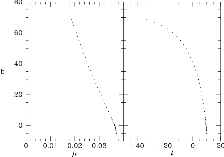
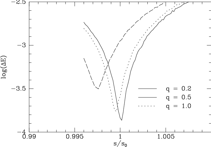
The right panel of Fig. 1 shows the track over the sky of an orbit that starts at galactic latitude and a distance as viewed from the Sun, which is on a circular orbit at . The left panel shows the magnitude of the proper motion along the orbit. The points in Fig. 2 show the rms variation in the energy of orbits that are reconstructed from the 42 data points shown in Fig. 1 for various assumed distances to the fiducial point and three trial potentials: the true potential, which has scale-length ratio and two less flattened potentials. The rms variation in has a sharp minimum at the true distance when the true potential is used, and higher minima when the wrong potential is used. The exquisite precision with which the distance can be determined from this plot is remarkable: better than three parts in .
In Fig. 2 the smallest value reached by the rms energy variation is significantly higher than the corresponding figure for the same orbit when line-of-sight velocities are used (Paper I). However, for other orbits smaller values of the rms variation in energy are obtained from proper-motion data; not surprisingly the data with the greatest diagnostic power varies with the nature of the orbit.
5 Conclusions
We have complemented the work of Paper I by showing that when proper motions can be measured along a section of a single orbit, the full phase-space coordinates for the orbit can be reconstructed as readily as is the case when line-of-sight velocities have been measured. However, we have also recovered a more powerful result: if the direction as well as the magnitude of the proper motions can be accurately measured, the three-dimensional geometry of the orbit can be recovered without assuming anything about the Galaxy’s gravitational potential. This reconstruction is possible because the Sun’s velocity must be responsible for the motion of stars perpendicular to the orbit, so from proper motion perpendicular to an orbit distances can be inferred that are as fundamental as conventional trigonometric parallaxes.
The extension of the work of Paper I to proper motions is useful because proper motions can be readily measured for the main-sequence stars that define the stream. These stars are typically so faint () that it is hard to obtain line-of-sight velocities of the requisite accuracy for large numbers of them.
In Paper II we show that even when line-of-sight velocities are available, a combination of observational errors and the fact that a tidal stream does not strictly follow an orbit make the task of determining whether a given potential is compatible with an observed stream complex. It proves necessary to search a multi-dimensional space of phase-space tracks that are compatible with the data for ones that are dynamically consistent orbits. A comparable search would be required when the data included proper motions rather than line-of-sight velocities. In a future paper we will extend to proper motions the techniques for handling this problem that are developed for line-of-sight velocities in Paper II.
Another interesting avenue is to determine the solar motion by treating it as an unknown when reconstructing orbits for several streams, using either line-of-sight velocities or proper motions, and choosing the value which allows a consistent interpretation of these streams. Recently Koposov et al. (2009) used a combination of line-of-sight velocities and proper motions for the GD-1 stream to constrain . Stronger constraints should be attainable by modelling several streams simultaneously.
Acknowledgments
We thank the anonymous referee for his/her suggestions. AE acknowledges the support of PPARC/STFC during preparation of this work.
References
- Belokurov et al. (2006a) Belokurov, V., Evans N.W., Irwin M.J., Hewett P.C., Wilkinson M.I., 2006a, ApJ, 637, L29
- Belokurov et al. (2006b) Belokurov, V., et al., (15 authors) 2006b, ApJ, 642, L137
- Belokurov et al. (2007) Belokurov, V., et al., (22 authors) 2007, ApJ, 658, 337
- Binney (2008) Binney J., 2008, MNRAS, 383, L47 (Paper I)
- Eyre & Binney (2009) Eyre A., Binney J., 2009, MNRAS, submitted (Paper II)
- Fellhauer et al. (2007) Fellhauer M., Evans N.W., Belokurov, V., Wilkinson M.I., Gilmore G., 2007, MNRAS, 380, 749
- Grillmair (2006) Grillmair C.J., 2006, ApJ, 651, L29
- Grillmair & Johnson (2006) Grillmair C.J., Johnson R., 2006, ApJ, 639, L17
- Grillmair & Dionatos (2006) Grillmair C.J., Dionatos, O., 2006, ApJ, 643, L17
- Grillmair et al. (2008) Grillmair C.J., Carlin J.L., Mejewski S.R., 2008, ApJ, 689, L117
- Johnston et al. (1996) Johnston K.V., Hernquist L., Bolte M., 1996, ApJ, 465, 278
- Jin & Lynden-Bell (2007) Jin S., Lynden-Bell D., 2007, MNRAS, 378, 64
- Koposov et al. (2009) Koposov S.E., Rix H.-W., Hogg D.W., 2009, ApJ, submitted
- Majewski et al. (2004) Majewski S.R., et al. 2004, AJ, 128, 245
- Miyamoto & Nagai (1975) Miyamoto M., Nagai R., 1975, PASJ, 27, 533
- Munn et al. (2004) Munn J.A., et al., 2004, AJ, 127, 3034
- Odenkirchen et al. (2002) Odenkirchen M., Grebel E.V., Dehnen W., Rix H.-W., Cudworth K.M., 2002, AJ, 124, 1497
- Odenkirchen et al. (2009) Odenkirchen M., Grebel E.K., Kayser A., Rix H.-W., Dehnen W., 2009, AJ, 137, 3378