1 Introduction
Quantum key distribution is an emerging technology that promises information-theoretic security, without computational infeasibility assumptions. Taking the classical BB84 protocol as an example, this one comprises the following steps:
1.
Alice sends randomly polarized photons to Bob
2.
Bob measures in a random polarization basis
3.
Bob keeps track of successful measurements
4.
Bob tells Alice the polarizer settings he used
5.
Alice tells Bob which settings have been correct
6.
Both discard all incorrect measurements
7.
Both map measurement results to a bitstring
8.
Both perform error correction
9.
Both perform privacy amplification
In a nutshell, the idea is to exploit photons as carriers of information due to their incapability of being copied. This renowned result is known as the no-cloning theorem [17 ] . Hence, any unauthorized access to the information encoded in the photons will result in an unnaturally high error rate, thus revealing the eavesdropping attempt eventually. The original protocol is found in [1 ] . A rigorous proof of security is provided in [11 ] , for instance.
We are particularly interested in step 8 of the BB84 protocol, in
which Alice and Bob locate and repair errors in their bit-strings. The process is known as reconciliation , and involves Alice
and Bob publicly exchanging parity bits in order to correct errors and distill identical keys. With each published parity bit, a piece of
information leaks out and becomes visible to the adversary, which is the reason why reconciliation is followed by
privacy amplification . Basically, this is the application of a strongly universal hash function on the output, in order to create dependencies of the final bits on the bits that the
adversary did not get any information about, thus sufficiently decreasing the adversary’s information. We shall not go into details
about the privacy amplification, and refer the reader to the literature on universal hashing
[13 , 14 , 4 ] as well as theoretical results about privacy amplification
[8 , 9 ] , and references therein for further information.
2 Interactive Error Correction
Let us pay closer attention to the error correction mechanism which has been proposed along with the experimental
implementation of BB84 [2 ] . Errors in physical transmission media often exhibit burst structures, that
is, a sequence of consecutive errors is more likely to occur than sparse scattering. Consequently, a popular trick is
to permute the bits in the string prior to the error correction in order to chop down long bursts into small pieces.
Ideally, this leaves an almost uniform pattern of erroneous bits in the result. This is the first step in a protocol
which has become known under the name Cascade .
After having agreed on a publicly known permutation of bits,
Alice and Bob take their shuffled strings and partition them into blocks of constant size k \mathchar 29035 [2 ] .
The problem of how errors are scattered across the raw key has been tackled on statistical grounds in [5 ] . The authors of this work assume a binomial distribution of errors within the blocks, which is later approximated by a Poisson-distribution.
We shall take a different route here, considering the process that induces the errors to be Poissonian, as well as adapting the initial block-size using a decision-theoretic approach. The authors of [5 ] do not provide a direct clue on how to choose an optimal block-size for partitioning. This is the gap we intend to close now. Before getting into details about how to cleverly choose the block-sizes, let us outline the remaining steps in the error correction process. This will highlight the room for improvement that an intelligent partitioning strategy can exploit.
Having split the string into blocks of equal size k \mathchar 29035 log ( k ) \log\delimiter 67273472\mathchar 29035\delimiter 84054785 1 1
Figure 1: Bisective search for errors
Example : The inherent problem with parity checking, which motivates the need for the repeated shuffling and
creation of larger blocks, can be illustrated as follows: assume that Alice and Bob share the following bit-strings,
with errors in Bob’s string being underlined,
Alice: 0 0 1 1 0 1 0 1 0 0 1 0 1 1 0 1 1 1 0 1 0 1 0 1 0 0 1 1 0 1 0 … Bob: 0 0 1 1 0 1 1 ¯ 1 0 0 1 0 1 1 0 1 0 0 ¯ 0 1 0 1 1 ¯ 1 1 ¯ 0 1 1 0 0 ¯ 0 … \begin{array}[]{rc}\text{Alice:}&\mathchar 28720\mathchar 28720\mathchar 28721\mathchar 28721\mathchar 28720\mathchar 28721\mathchar 28720\mathchar 28721\mathchar 28720\mathchar 28720\mathchar 28721\mathchar 28720\mathchar 28721\mathchar 28721\mathchar 28720\mathchar 28721\mathchar 28721\mathchar 28721\mathchar 28720\mathchar 28721\mathchar 28720\mathchar 28721\mathchar 28720\mathchar 28721\mathchar 28720\mathchar 28720\mathchar 28721\mathchar 28721\mathchar 28720\mathchar 28721\mathchar 28720\ldots\\
\text{Bob:}&\mathchar 28720\mathchar 28720\mathchar 28721\mathchar 28721\mathchar 28720\mathchar 28721\underline{\mathchar 28721}\mathchar 28721\mathchar 28720\mathchar 28720\mathchar 28721\mathchar 28720\mathchar 28721\mathchar 28721\mathchar 28720\mathchar 28721\underline{\mathchar 28720\mathchar 28720}\mathchar 28720\mathchar 28721\mathchar 28720\mathchar 28721\underline{\mathchar 28721}\mathchar 28721\underline{\mathchar 28721}\mathchar 28720\mathchar 28721\mathchar 28721\mathchar 28720\underline{\mathchar 28720}\mathchar 28720\ldots\\
\end{array}
Partitioning into blocks of equal size and comparing parities of blocks will let some errors go undisclosed (parity
bits are shown in the two middle rows; agreeing parities hiding existing errors are underlined):
Alice: 0 0 1 1 0 ⏟ 0 | 1 0 1 0 0 ⏟ 0 | 1 0 1 1 0 ⏟ 1 | 1 1 1 0 1 ⏟ 0 | 0 1 0 1 0 ⏟ 0 | 0 1 1 0 1 ⏟ 0 | 0 … Bob: 0 0 1 1 0 ⏞ 0 | 1 1 ¯ 1 0 0 ⏞ 1 | 1 0 1 1 0 ⏞ 1 | 1 0 0 ¯ 0 1 ⏞ 0 ¯ | 0 1 1 ¯ 1 1 ¯ ⏞ 0 ¯ | 0 1 1 0 0 ¯ ⏞ 1 | 1 … \begin{array}[]{rc}\text{Alice:}&\underbrace{\mathchar 28720\mathchar 28720\mathchar 28721\mathchar 28721\mathchar 28720}_{\mathchar 28720}\delimiter 2532108\underbrace{\mathchar 28721\mathchar 28720\mathchar 28721\mathchar 28720\mathchar 28720}_{\mathchar 28720}\delimiter 2532108\underbrace{\mathchar 28721\mathchar 28720\mathchar 28721\mathchar 28721\mathchar 28720}_{\mathchar 28721}\delimiter 2532108\underbrace{\mathchar 28721\mathchar 28721\mathchar 28721\mathchar 28720\mathchar 28721}_{\mathchar 28720}\delimiter 2532108\underbrace{\mathchar 28720\mathchar 28721\mathchar 28720\mathchar 28721\mathchar 28720}_{\mathchar 28720}\delimiter 2532108\underbrace{\mathchar 28720\mathchar 28721\mathchar 28721\mathchar 28720\mathchar 28721}_{\mathchar 28720}\delimiter 2532108\mathchar 28720\ldots\\
\text{Bob:}&\overbrace{\mathchar 28720\mathchar 28720\mathchar 28721\mathchar 28721\mathchar 28720}^{\mathchar 28720}\delimiter 2532108\overbrace{\mathchar 28721\underline{\mathchar 28721}\mathchar 28721\mathchar 28720\mathchar 28720}^{\mathchar 28721}\delimiter 2532108\overbrace{\mathchar 28721\mathchar 28720\mathchar 28721\mathchar 28721\mathchar 28720}^{\mathchar 28721}\delimiter 2532108\overbrace{\mathchar 28721\underline{\mathchar 28720\mathchar 28720}\mathchar 28720\mathchar 28721}^{\underline{\mathchar 28720}}\delimiter 2532108\overbrace{\mathchar 28720\mathchar 28721\underline{\mathchar 28721}\mathchar 28721\underline{\mathchar 28721}}^{\underline{\mathchar 28720}}\delimiter 2532108\overbrace{\mathchar 28720\mathchar 28721\mathchar 28721\mathchar 28720\underline{\mathchar 28720}}^{\mathchar 28721}\delimiter 2532108\mathchar 28721\ldots\end{array}
Sparing the shuffling of bits will save some errors from discovery, since two blocks (in this example, the 4th and 5th)
with even number of errors can form a larger block with an even number of errors again. Therefore, permuting the bits
is inevitable to avoid such an undesirable coincidence.
Since the error correction up to now may be ineffective, as still having missed some errors, Alice and Bob continue by
comparing parities of random subsets of bits they publicly agree on. Upon parity mismatch, a bisective search similarly
as above is performed to find and erase the error. In order to avoid information leaking to the adversary, the last bit
from each random subset is deleted. This deletion is also done after comparing parities of blocks in the previous steps, for the same reason.
The point at which almost all errors have been removed is detected by counting the number of successful comparisons
after having discovered the last error. After a sufficient number of successful trials (20 is the number proposed in
[2 ] ), the strings are accepted as identical, regarding the probability of errors remaining undetected
as negligible.
The protocol Cascade is based on this procedure and has been introduced in a later paper [3 ] ,
which presented improvements to the original reconciliation protocol sketched above. Among the changes is the removal
of the bit-deletion step for the sake of detecting more errors faster, so the task of information leakage reduction is
shifted to the privacy amplification stage. The naming stems from the strategy of increasing sizes of blocks in the
first stages of the protocol. Although a theoretical analysis of the protocol is provided, the authors of
[3 ] , as well as those of [2 ] abstain from an analytical treatment of block-size
choices. Nevertheless, they give a simple heuristic based on estimating the error frequency by direct comparison of a
random sample of bits is provided in [2 ] . These bits have to be sacrificed for the sake of privacy too,
if that approach is adopted. To summarize, the error correction protocol in charge of current QKD implementations relies on
Assumption 1
A block-size exists, such that by partitioning the raw key into blocks of that given size, each block contains at most one error.
It is this assumption that we seek to support by our upcoming theoretical considerations.
3 An error scattering model
We choose the Poisson process as the natural model for errors that occur within a sequence of bits that can be arbitrarily long.
Definition 2 (Poisson process [10 ] )
A Poisson process is a family of discrete counting measures
{ N ( t ) : t ≥ 0 } \left\{\mathchar 29006\delimiter 67273472\mathchar 29044\delimiter 84054785\mathchar 12346\mathchar 29044\mathchar 12821\mathchar 28720\right\}
1.
N ( 0 ) = 0 \mathchar 29006\delimiter 67273472\mathchar 28720\delimiter 84054785\mathchar 12349\mathchar 28720 (no events yet at the beginning).
2.
The process has independent increments.
3.
The number of events in any interval of length Δ t \mathchar 28673\mathchar 29044 is Poisson distributed with mean λ Δ t \mathchar 28949\mathchar 28673\mathchar 29044 . That is, for all t , Δ t ≥ 0 \mathchar 29044\mathchar 24891\mathchar 28673\mathchar 29044\mathchar 12821\mathchar 28720 ,
Pr { N ( t + Δ t ) − N ( t ) = n } = ( λ ⋅ Δ t ) n n ! e − UNKNOWN ⋅ UNKNOWN t , n = 0 , 1 , 2 , … . \Pr\left\{\mathchar 29006\delimiter 67273472\mathchar 29044\mathchar 8235\mathchar 28673\mathchar 29044\delimiter 84054785\mathchar 8704\mathchar 29006\delimiter 67273472\mathchar 29044\delimiter 84054785\mathchar 12349\mathchar 29038\right\}\mathchar 12349{{\delimiter 67273472\mathchar 28949\mathchar 8705\mathchar 28673\mathchar 29044\delimiter 84054785^{\mathchar 29038}\over\mathchar 29038\mathchar 24609}}\mathchar 29029^{\mathchar 8704\mathchar 28949\mathchar 8705\mathchar 28673\mathchar 29044}\mathchar 24891\quad\mathchar 29038\mathchar 12349\mathchar 28720\mathchar 24891\mathchar 28721\mathchar 24891\mathchar 28722\mathchar 24891\ldots\mathchar 314
In other words, the expected number of events linearly increases with the length of the block.
Our Poisson process model N ( t ) \mathchar 29006\delimiter 67273472\mathchar 29044\delimiter 84054785 t \mathchar 29044 Δ t \mathchar 28673\mathchar 29044 1 \mathchar 28721 λ \mathchar 28949
Assume that this intensity-parameter remains constant over a unit of time, and denote it by
Λ ∈ [ 0 , ∞ ) \mathchar 28675\mathchar 12850\delimiter 67482370\mathchar 28720\mathchar 24891\mathchar 561\delimiter 84054785 2 2 T \mathchar 29012 a = 1 0 \mathchar 29025\mathchar 12349\mathchar 28721\mathchar 28720 b = 2 \mathchar 29026\mathchar 12349\mathchar 28722
Figure 2: Example error intensity parameter process
The probability of exactly k \mathchar 29035 X \mathchar 29016
Pr { X = k } = ∫ 0 ∞ Pr { X = k | λ = x } ⏟
Poisson distributed with parameter λ Pr { λ = x } ⏟
intensity parameter d x . \Pr\left\{\mathchar 29016\mathchar 12349\mathchar 29035\right\}\mathchar 12349\mathchar 4946\nolimits_{\mathchar 28720}^{\mathchar 561}\underbrace{\Pr\left\{\mathchar 29016\mathchar 12349\mathchar 29035\delimiter 2532108\mathchar 28949\mathchar 12349\mathchar 29048\right\}}_{\text{\shortstack{Poisson distributed\\
with parameter $\mathchar 28949$}}}\underbrace{\Pr\left\{\mathchar 28949\mathchar 12349\mathchar 29048\right\}}_{\text{\shortstack{intensity\\
parameter}}}\mathchar 29028\mathchar 29048\mathchar 314 (1)
For the intensity-parameter, we assume a gamma-distribution. This choice is intuitively reasonable, as this class is flexible and supported on the nonnegative real line. Plugging into (1
f ( λ | a , b ) = { b a UNKNOWN ( a ) UNKNOWN a − 1 e − b UNKNOWN , UNKNOWN ≥ 0 0 , UNKNOWN < 0 , . \mathchar 29030\delimiter 67273472\mathchar 28949\delimiter 2532108\mathchar 29025\mathchar 24891\mathchar 29026\delimiter 84054785\mathchar 12349\left\{\begin{array}[]{ll}{{\mathchar 29026^{\mathchar 29025}\over\mathchar 28672\delimiter 67273472\mathchar 29025\delimiter 84054785}}\mathchar 28949^{\mathchar 29025\mathchar 8704\mathchar 28721}\mathchar 29029^{\mathchar 8704\mathchar 29026\mathchar 28949}\mathchar 24891&\mathchar 28949\mathchar 12821\mathchar 28720\\
\mathchar 28720\mathchar 24891&\mathchar 28949\mathchar 12604\mathchar 28720\mathchar 24891\end{array}\right\mathchar 314
and the density of the Poisson-distribution, which is
f ( k | λ ) = λ k k ! e − UNKNOWN , \mathchar 29030\delimiter 67273472\mathchar 29035\delimiter 2532108\mathchar 28949\delimiter 84054785\mathchar 12349{{\mathchar 28949^{\mathchar 29035}\over\mathchar 29035\mathchar 24609}}\mathchar 29029^{\mathchar 8704\mathchar 28949}\mathchar 24891
we find
Pr { X = k } \displaystyle\Pr\left\{\mathchar 29016\mathchar 12349\mathchar 29035\right\} b a k ! Γ ( a ) ∫ 0 ∞ x k + a − 1 e − x ( b + 1 ) 𝑑 x \displaystyle{{\mathchar 29026^{\mathchar 29025}\over\mathchar 29035\mathchar 24609\mathchar 28672\delimiter 67273472\mathchar 29025\delimiter 84054785}}\mathchar 4946\nolimits_{\mathchar 28720}^{\mathchar 561}\mathchar 29048^{\mathchar 29035\mathchar 8235\mathchar 29025\mathchar 8704\mathchar 28721}\mathchar 29029^{\mathchar 8704\mathchar 29048\delimiter 67273472\mathchar 29026\mathchar 8235\mathchar 28721\delimiter 84054785}\mathchar 29028\mathchar 29048 (2)
b a UNKNOWN ( k + a ) k ! ( b + 1 ) k + a Γ ( a ) , \displaystyle{{\mathchar 29026^{\mathchar 29025}\mathchar 28672\delimiter 67273472\mathchar 29035\mathchar 8235\mathchar 29025\delimiter 84054785\over\mathchar 29035\mathchar 24609\delimiter 67273472\mathchar 29026\mathchar 8235\mathchar 28721\delimiter 84054785^{\mathchar 29035\mathchar 8235\mathchar 29025}\mathchar 28672\delimiter 67273472\mathchar 29025\delimiter 84054785}}\mathchar 24891
where Γ \mathchar 28672 3 3 a = 1 0 \mathchar 29025\mathchar 12349\mathchar 28721\mathchar 28720 b = 2 \mathchar 29026\mathchar 12349\mathchar 28722
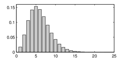
Figure 3: Example of error probabilities under Cox process error scattering
This discrete probability density has a closed form expression for its first moment. The expected number of errors per
time unit for this model is
𝔼 X = ∑ k = 0 ∞ k ⋅ Pr { k errors per time unit } = a b . \mathds{\mathchar 28997}\mathchar 29016\mathchar 12349\mathchar 4944\displaylimits_{\mathchar 29035\mathchar 12349\mathchar 28720}^{\mathchar 561}\mathchar 29035\mathchar 8705\Pr\left\{\text{$\mathchar 29035$ errors per time unit}\right\}\mathchar 12349{{\mathchar 29025\over\mathchar 29026}}\mathchar 314 (3)
So far, we are almost done, because Assumption 1 Δ t \mathchar 28673\mathchar 29044 a b ⋅ ( Δ t ) {{\mathchar 29025\over\mathchar 29026}}\mathchar 8705\delimiter 67273472\mathchar 28673\mathchar 29044\delimiter 84054785 f \mathchar 29030 n \mathchar 29038 Δ t \mathchar 28673\mathchar 29044 f ⋅ Δ t = n \mathchar 29030\mathchar 8705\mathchar 28673\mathchar 29044\mathchar 12349\mathchar 29038 a b ⋅ n f = 1 {{\mathchar 29025\over\mathchar 29026}}\mathchar 8705{{\mathchar 29038\over\mathchar 29030}}\mathchar 12349\mathchar 28721
initial block-size n ≈ f a / b , \text{initial block-size }\mathchar 29038\mathchar 12825{{\mathchar 29030\over\mathchar 29025\delimiter 1299214\mathchar 29026}}\mathchar 24891
which is the block-size (in bits) that the Poisson process gives us. Observe that we have a constant block-size again.
The only difference to the original Cascade variant is that it originates from a probabilistic model, rather than from
pure intuition.
All calculations above were done with the Maple software [6 ] . The density of X \mathchar 29016
Using the density (2 m \mathchar 29037
Pr { X > m } = b a ( a ) m + 1 ( m + 1 ) ! ( b + 1 ) a + m + 1 ⋅ F 1 2 ( 1 , m + a + 1 m + 2 1 b + 1 ) , \Pr\left\{\mathchar 29016\mathchar 12606\mathchar 29037\right\}\mathchar 12349{{\mathchar 29026^{\mathchar 29025}\delimiter 67273472\mathchar 29025\delimiter 84054785_{\mathchar 29037\mathchar 8235\mathchar 28721}\over\delimiter 67273472\mathchar 29037\mathchar 8235\mathchar 28721\delimiter 84054785\mathchar 24609\delimiter 67273472\mathchar 29026\mathchar 8235\mathchar 28721\delimiter 84054785^{\mathchar 29025\mathchar 8235\mathchar 29037\mathchar 8235\mathchar 28721}}}\mathchar 8705{{}_{\mathchar 28722}}\mathchar 28998_{\mathchar 28721}\!\!\left\delimiter 67273472\!\!\!\!\begin{array}[]{c|c}\begin{array}[]{c}\mathchar 28721\mathchar 24891\mathchar 29037\mathchar 8235\mathchar 29025\mathchar 8235\mathchar 28721\\
\mathchar 29037\mathchar 8235\mathchar 28722\end{array}&{{\mathchar 28721\over\mathchar 29026\mathchar 8235\mathchar 28721}}\end{array}\!\!\!\!\right\delimiter 84054785\mathchar 24891 (4)
where a , b > 0 \mathchar 29025\mathchar 24891\mathchar 29026\mathchar 12606\mathchar 28720 F 1 2 {}_{\mathchar 28722}\mathchar 28998_{\mathchar 28721} 9 ( a ) m \delimiter 67273472\mathchar 29025\delimiter 84054785_{\mathchar 29037} 10
Since error correction in the way used with quantum key distribution relies on public parity comparisons, the
event of missing an error is equal to the event of having an even number of errors. The probability that the
parity check can indicate an error, is calculated as follows (the derivation is shown in Section 4
Pr { odd number of errors } = p odd = 1 2 [ 1 − ( b b + 1 ) a ] . \Pr\left\{\text{odd number of errors}\right\}\mathchar 12349\mathchar 29040_{\text{odd}}\mathchar 12349{{\mathchar 28721\over\mathchar 28722}}\left\delimiter 67482370\mathchar 28721\mathchar 8704\left\delimiter 67273472{{\mathchar 29026\over\mathchar 29026\mathchar 8235\mathchar 28721}}\right\delimiter 84054785^{\mathchar 29025}\right\delimiter 84267779\mathchar 314 (5)
For a finite string of length 2 m + 1 \mathchar 28722\mathchar 29037\mathchar 8235\mathchar 28721
p = p odd − C ( a , b , m ) ⋅ F 2 3 ( 1 , m + 2 + a 2 , m + 3 2 + a 2 m + 2 , m + 5 2 1 ( b + 1 ) 2 ) , \mathchar 29040\mathchar 12349\mathchar 29040_{\text{odd}}\mathchar 8704\mathchar 28995\delimiter 67273472\mathchar 29025\mathchar 24891\mathchar 29026\mathchar 24891\mathchar 29037\delimiter 84054785\mathchar 8705{{}_{\mathchar 28723}}\mathchar 28998_{\mathchar 28722}\!\!\left\delimiter 67273472\!\!\!\!\begin{array}[]{c|c}\begin{array}[]{c}\mathchar 28721\mathchar 24891\mathchar 29037\mathchar 8235\mathchar 28722\mathchar 8235{{\mathchar 29025\over\mathchar 28722}}\mathchar 24891\mathchar 29037\mathchar 8235{{\mathchar 28723\over\mathchar 28722}}\mathchar 8235{{\mathchar 29025\over\mathchar 28722}}\\
\mathchar 29037\mathchar 8235\mathchar 28722\mathchar 24891\mathchar 29037\mathchar 8235{{\mathchar 28725\over\mathchar 28722}}\end{array}&{{\mathchar 28721\over\delimiter 67273472\mathchar 29026\mathchar 8235\mathchar 28721\delimiter 84054785^{\mathchar 28722}}}\end{array}\!\!\!\!\right\delimiter 84054785\mathchar 24891 (6)
where
C ( a , b , m ) = b a Γ ( 2 m + 3 + a ) UNKNOWN ( a ) ( 2 m + 3 ) ! ( b + 1 ) 2 m + 3 + a . \mathchar 28995\delimiter 67273472\mathchar 29025\mathchar 24891\mathchar 29026\mathchar 24891\mathchar 29037\delimiter 84054785\mathchar 12349{{\mathchar 29026^{\mathchar 29025}\mathchar 28672\delimiter 67273472\mathchar 28722\mathchar 29037\mathchar 8235\mathchar 28723\mathchar 8235\mathchar 29025\delimiter 84054785\over\mathchar 28672\delimiter 67273472\mathchar 29025\delimiter 84054785\delimiter 67273472\mathchar 28722\mathchar 29037\mathchar 8235\mathchar 28723\delimiter 84054785\mathchar 24609\delimiter 67273472\mathchar 29026\mathchar 8235\mathchar 28721\delimiter 84054785^{\mathchar 28722\mathchar 29037\mathchar 8235\mathchar 28723\mathchar 8235\mathchar 29025}}}\mathchar 314
The previous results are an appealing tool for a proper choice of the parameters if an error-correcting code shall be used with the scheme. Employing classical error correction
mechanisms may not work well, since our wish is to detect eavesdropping via a raised error rate. Therefore, we cannot
adopt any assumption on how many errors will occur at maximum, and classical error-correcting codes can no longer be
used for that matter. However, if the probability of seeing more than m \mathchar 29037
4 Proofs
This section is dedicated to proving equations (3 4 5 6
For the probability distribution function let us first substitute c : = b + 1 \mathchar 29027\mathchar 12346\mathchar 12349\mathchar 29026\mathchar 8235\mathchar 28721 2
F ( m ) = Pr { X ≤ m } = ∑ k = 0 m Pr { X = k } \displaystyle\mathchar 28998\delimiter 67273472\mathchar 29037\delimiter 84054785\mathchar 12349\Pr\left\{\mathchar 29016\mathchar 12820\mathchar 29037\right\}\mathchar 12349\mathchar 4944\displaylimits_{\mathchar 29035\mathchar 12349\mathchar 28720}^{\mathchar 29037}\Pr\left\{\mathchar 29016\mathchar 12349\mathchar 29035\right\} ∑ k = 0 m b a UNKNOWN ( k + a ) k ! ( b + 1 ) k + a Γ ( a ) \displaystyle\mathchar 4944\displaylimits_{\mathchar 29035\mathchar 12349\mathchar 28720}^{\mathchar 29037}{{\mathchar 29026^{\mathchar 29025}\mathchar 28672\delimiter 67273472\mathchar 29035\mathchar 8235\mathchar 29025\delimiter 84054785\over\mathchar 29035\mathchar 24609\delimiter 67273472\mathchar 29026\mathchar 8235\mathchar 28721\delimiter 84054785^{\mathchar 29035\mathchar 8235\mathchar 29025}\mathchar 28672\delimiter 67273472\mathchar 29025\delimiter 84054785}} (7)
b a ( b + 1 ) a Γ ( a ) ∑ k = 0 m UNKNOWN ( k + a ) k ! ( b + 1 ) k \displaystyle{{\mathchar 29026^{\mathchar 29025}\over\delimiter 67273472\mathchar 29026\mathchar 8235\mathchar 28721\delimiter 84054785^{\mathchar 29025}\mathchar 28672\delimiter 67273472\mathchar 29025\delimiter 84054785}}\mathchar 4944\displaylimits_{\mathchar 29035\mathchar 12349\mathchar 28720}^{\mathchar 29037}{{\mathchar 28672\delimiter 67273472\mathchar 29035\mathchar 8235\mathchar 29025\delimiter 84054785\over\mathchar 29035\mathchar 24609\delimiter 67273472\mathchar 29026\mathchar 8235\mathchar 28721\delimiter 84054785^{\mathchar 29035}}}
∑ k = 0 m UNKNOWN ( k + a ) k ! c k . \displaystyle\mathchar 4944\displaylimits_{\mathchar 29035\mathchar 12349\mathchar 28720}^{\mathchar 29037}{{\mathchar 28672\delimiter 67273472\mathchar 29035\mathchar 8235\mathchar 29025\delimiter 84054785\over\mathchar 29035\mathchar 24609\mathchar 29027^{\mathchar 29035}}}\mathchar 314
Using the Maple software [6 ] , we obtain for the finite sum (7
G ( m ) = ∑ k = 0 m Γ ( k + a ) k ! c k = Γ ( a ) ( c − 1 c ) a − Γ ( m + 1 + a ) ⋅ F 1 2 ( 1 , m + a + 1 m + 2 1 c ) ( m + 1 ) ! c m + 1 , \mathchar 28999\delimiter 67273472\mathchar 29037\delimiter 84054785\mathchar 12349\mathchar 4944\displaylimits_{\mathchar 29035\mathchar 12349\mathchar 28720}^{\mathchar 29037}{{\mathchar 28672\delimiter 67273472\mathchar 29035\mathchar 8235\mathchar 29025\delimiter 84054785\over\mathchar 29035\mathchar 24609\mathchar 29027^{\mathchar 29035}}}\mathchar 12349{{\mathchar 28672\delimiter 67273472\mathchar 29025\delimiter 84054785\over\left\delimiter 67273472{{\mathchar 29027\mathchar 8704\mathchar 28721\over\mathchar 29027}}\right\delimiter 84054785^{\mathchar 29025}}}\mathchar 8704{{\mathchar 28672\delimiter 67273472\mathchar 29037\mathchar 8235\mathchar 28721\mathchar 8235\mathchar 29025\delimiter 84054785\mathchar 8705{{}_{\mathchar 28722}}\mathchar 28998_{\mathchar 28721}\!\!\left\delimiter 67273472\!\!\!\!\begin{array}[]{c|c}\begin{array}[]{c}\mathchar 28721\mathchar 24891\mathchar 29037\mathchar 8235\mathchar 29025\mathchar 8235\mathchar 28721\\
\mathchar 29037\mathchar 8235\mathchar 28722\end{array}&{{\mathchar 28721\over\mathchar 29027}}\end{array}\!\!\!\!\right\delimiter 84054785\over\delimiter 67273472\mathchar 29037\mathchar 8235\mathchar 28721\delimiter 84054785\mathchar 24609\mathchar 29027^{\mathchar 29037\mathchar 8235\mathchar 28721}}}\mathchar 24891 (8)
where
F q p ( a 1 , … , a p b 1 , … , b q x ) : = ∑ k = 0 ∞ ( a 1 ) k ( a 2 ) k ⋅ ⋅ ⋅ ( a p ) k ( b 1 ) k ( b 2 ) k ⋅ ⋅ ⋅ ( b q ) k x k k ! {{}_{\mathchar 29040}}\mathchar 28998_{\mathchar 29041}\!\!\left\delimiter 67273472\!\!\!\!\begin{array}[]{c|c}\begin{array}[]{c}\mathchar 29025_{\mathchar 28721}\mathchar 24891\ldots\mathchar 24891\mathchar 29025_{\mathchar 29040}\\
\mathchar 29026_{\mathchar 28721}\mathchar 24891\ldots\mathchar 24891\mathchar 29026_{\mathchar 29041}\end{array}&\mathchar 29048\end{array}\!\!\!\!\right\delimiter 84054785\mathchar 12346\mathchar 12349\mathchar 4944\displaylimits_{\mathchar 29035\mathchar 12349\mathchar 28720}^{\mathchar 561}{{\delimiter 67273472\mathchar 29025_{\mathchar 28721}\delimiter 84054785_{\mathchar 29035}\delimiter 67273472\mathchar 29025_{\mathchar 28722}\delimiter 84054785_{\mathchar 29035}\mathinner{\mathpunct{\mathchar 513}\mathpunct{\mathchar 513}\mathpunct{\mathchar 513}}\delimiter 67273472\mathchar 29025_{\mathchar 29040}\delimiter 84054785_{\mathchar 29035}\over\delimiter 67273472\mathchar 29026_{\mathchar 28721}\delimiter 84054785_{\mathchar 29035}\delimiter 67273472\mathchar 29026_{\mathchar 28722}\delimiter 84054785_{\mathchar 29035}\mathinner{\mathpunct{\mathchar 513}\mathpunct{\mathchar 513}\mathpunct{\mathchar 513}}\delimiter 67273472\mathchar 29026_{\mathchar 29041}\delimiter 84054785_{\mathchar 29035}}}{{\mathchar 29048^{\mathchar 29035}\over\mathchar 29035\mathchar 24609}} (9)
is the generalized hypergeometric function, and
( x ) n : = Γ ( x + n ) UNKNOWN ( x ) = x ( x + 1 ) ( x + 2 ) ⋅ ⋅ ⋅ ( x + n − 1 ) \delimiter 67273472\mathchar 29048\delimiter 84054785_{\mathchar 29038}\mathchar 12346\mathchar 12349{{\mathchar 28672\delimiter 67273472\mathchar 29048\mathchar 8235\mathchar 29038\delimiter 84054785\over\mathchar 28672\delimiter 67273472\mathchar 29048\delimiter 84054785}}\mathchar 12349\mathchar 29048\delimiter 67273472\mathchar 29048\mathchar 8235\mathchar 28721\delimiter 84054785\delimiter 67273472\mathchar 29048\mathchar 8235\mathchar 28722\delimiter 84054785\mathinner{\mathpunct{\mathchar 513}\mathpunct{\mathchar 513}\mathpunct{\mathchar 513}}\delimiter 67273472\mathchar 29048\mathchar 8235\mathchar 29038\mathchar 8704\mathchar 28721\delimiter 84054785 (10)
is the Pochhammer symbol. Useful special cases are ( 1 ) k = k ! \delimiter 67273472\mathchar 28721\delimiter 84054785_{\mathchar 29035}\mathchar 12349\mathchar 29035\mathchar 24609 ( 2 ) k = ( k + 1 ) ! \delimiter 67273472\mathchar 28722\delimiter 84054785_{\mathchar 29035}\mathchar 12349\delimiter 67273472\mathchar 29035\mathchar 8235\mathchar 28721\delimiter 84054785\mathchar 24609
It is important to notice that the parameters of the Gamma density used for deriving the density
(2 a , b > 0 \mathchar 29025\mathchar 24891\mathchar 29026\mathchar 12606\mathchar 28720 0 ≤ 1 c = 1 b + 1 < 1 \mathchar 28720\mathchar 12820{{\mathchar 28721\over\mathchar 29027}}\mathchar 12349{{\mathchar 28721\over\mathchar 29026\mathchar 8235\mathchar 28721}}\mathchar 12604\mathchar 28721 8 [12 ] ). This is crucial for the permission to rearrange
the infinite sums in later stages of the upcoming derivation.
We verify expression (8 m = 0 \mathchar 29037\mathchar 12349\mathchar 28720 9
a [ F 1 2 ( 1 , 1 + a 2 1 c ) ] \displaystyle\mathchar 29025\left\delimiter 67482370{{}_{\mathchar 28722}}\mathchar 28998_{\mathchar 28721}\!\!\left\delimiter 67273472\!\!\!\!\begin{array}[]{c|c}\begin{array}[]{c}\mathchar 28721\mathchar 24891\mathchar 28721\mathchar 8235\mathchar 29025\\
\mathchar 28722\end{array}&{{\mathchar 28721\over\mathchar 29027}}\end{array}\!\!\!\!\right\delimiter 84054785\right\delimiter 84267779 a ∑ k = 0 ∞ ( 1 ) k ( 1 + a ) k ( 2 ) k 1 k ! c k \displaystyle\mathchar 29025\mathchar 4944\displaylimits_{\mathchar 29035\mathchar 12349\mathchar 28720}^{\mathchar 561}{{\delimiter 67273472\mathchar 28721\delimiter 84054785_{\mathchar 29035}\delimiter 67273472\mathchar 28721\mathchar 8235\mathchar 29025\delimiter 84054785_{\mathchar 29035}\over\delimiter 67273472\mathchar 28722\delimiter 84054785_{\mathchar 29035}}}{{\mathchar 28721\over\mathchar 29035\mathchar 24609\mathchar 29027^{\mathchar 29035}}}
∑ k = 0 ∞ ( a ) k + 1 ( k + 1 ) ! 1 c k \displaystyle\mathchar 4944\displaylimits_{\mathchar 29035\mathchar 12349\mathchar 28720}^{\mathchar 561}{{\delimiter 67273472\mathchar 29025\delimiter 84054785_{\mathchar 29035\mathchar 8235\mathchar 28721}\over\delimiter 67273472\mathchar 29035\mathchar 8235\mathchar 28721\delimiter 84054785\mathchar 24609}}{{\mathchar 28721\over\mathchar 29027^{\mathchar 29035}}}
c ∑ k = 1 ∞ ( a ) k k ! 1 c k . \displaystyle\mathchar 29027\mathchar 4944\displaylimits_{\mathchar 29035\mathchar 12349\mathchar 28721}^{\mathchar 561}{{\delimiter 67273472\mathchar 29025\delimiter 84054785_{\mathchar 29035}\over\mathchar 29035\mathchar 24609}}{{\mathchar 28721\over\mathchar 29027^{\mathchar 29035}}}\mathchar 314
The last series can be written in the form
∑ k = 1 ∞ ( a ) k k ! α k 1 c k = − 1 + ∑ k = 0 ∞ ( a ) k k ! α k 1 c k \mathchar 4944\displaylimits_{\mathchar 29035\mathchar 12349\mathchar 28721}^{\mathchar 561}{{\delimiter 67273472\mathchar 29025\delimiter 84054785_{\mathchar 29035}\over\mathchar 29035\mathchar 24609}}\mathchar 28939_{\mathchar 29035}{{\mathchar 28721\over\mathchar 29027^{\mathchar 29035}}}\mathchar 12349\mathchar 8704\mathchar 28721\mathchar 8235\mathchar 4944\displaylimits_{\mathchar 29035\mathchar 12349\mathchar 28720}^{\mathchar 561}{{\delimiter 67273472\mathchar 29025\delimiter 84054785_{\mathchar 29035}\over\mathchar 29035\mathchar 24609}}\mathchar 28939_{\mathchar 29035}{{\mathchar 28721\over\mathchar 29027^{\mathchar 29035}}} (13)
with coefficients α k = 1 \mathchar 28939_{\mathchar 29035}\mathchar 12349\mathchar 28721 k \mathchar 29035 [7 , 16 , 15 ] ),
∑ k = 0 ∞ ( a ) k k ! α k z k = ( 1 − z ) − a ∑ k = 0 ∞ ( a ) k k ! Δ k α 0 ( z 1 − z ) k , \mathchar 4944\displaylimits_{\mathchar 29035\mathchar 12349\mathchar 28720}^{\mathchar 561}{{\delimiter 67273472\mathchar 29025\delimiter 84054785_{\mathchar 29035}\over\mathchar 29035\mathchar 24609}}\mathchar 28939_{\mathchar 29035}\mathchar 29050^{\mathchar 29035}\mathchar 12349\delimiter 67273472\mathchar 28721\mathchar 8704\mathchar 29050\delimiter 84054785^{\mathchar 8704\mathchar 29025}\mathchar 4944\displaylimits_{\mathchar 29035\mathchar 12349\mathchar 28720}^{\mathchar 561}{{\delimiter 67273472\mathchar 29025\delimiter 84054785_{\mathchar 29035}\over\mathchar 29035\mathchar 24609}}\mathchar 28673^{\mathchar 29035}\mathchar 28939_{\mathchar 28720}\left\delimiter 67273472{{\mathchar 29050\over\mathchar 28721\mathchar 8704\mathchar 29050}}\right\delimiter 84054785^{\mathchar 29035}\mathchar 24891 (14)
with the forward difference Δ n α 0 \mathchar 28673^{\mathchar 29038}\mathchar 28939_{\mathchar 28720}
Δ n α 0 = ∑ i = 0 n ( − 1 ) i Γ 6 7 2 7 3 4 7 2 n i Γ 8 4 0 5 4 7 8 5 α n − i . \mathchar 28673^{\mathchar 29038}\mathchar 28939_{\mathchar 28720}\mathchar 12349\mathchar 4944\displaylimits_{\mathchar 29033\mathchar 12349\mathchar 28720}^{\mathchar 29038}\delimiter 67273472\mathchar 8704\mathchar 28721\delimiter 84054785^{\mathchar 29033}{{\mathchar 29038\abovewithdelims( ) 0.0pt\mathchar 29033}}\mathchar 28939_{\mathchar 29038\mathchar 8704\mathchar 29033}\mathchar 314 (15)
Expression (15
Δ n a 0 = ∑ i = 0 n ( − 1 ) i Γ 6 7 2 7 3 4 7 2 n i Γ 8 4 0 5 4 7 8 5 1 n − i = { ( − 1 + 1 ) n = 0 , for n > 0 ( − 1 ) 0 Γ 6 7 2 7 3 4 7 2 0 0 Γ 8 4 0 5 4 7 8 5 1 0 = 1 , for n = 0 . . \mathchar 28673^{\mathchar 29038}\mathchar 29025_{\mathchar 28720}\mathchar 12349\mathchar 4944\displaylimits_{\mathchar 29033\mathchar 12349\mathchar 28720}^{\mathchar 29038}\delimiter 67273472\mathchar 8704\mathchar 28721\delimiter 84054785^{\mathchar 29033}{{\mathchar 29038\abovewithdelims( ) 0.0pt\mathchar 29033}}\mathchar 28721^{\mathchar 29038\mathchar 8704\mathchar 29033}\mathchar 12349\left\{\begin{array}[]{ll}\delimiter 67273472\mathchar 8704\mathchar 28721\mathchar 8235\mathchar 28721\delimiter 84054785^{\mathchar 29038}\mathchar 12349\mathchar 28720\mathchar 24891&\hbox{for }\mathchar 29038\mathchar 12606\mathchar 28720\\
\delimiter 67273472\mathchar 8704\mathchar 28721\delimiter 84054785^{\mathchar 28720}{{\mathchar 28720\abovewithdelims( ) 0.0pt\mathchar 28720}}\mathchar 28721^{\mathchar 28720}\mathchar 12349\mathchar 28721\mathchar 24891&\hbox{for }\mathchar 29038\mathchar 12349\mathchar 28720\mathchar 314\end{array}\right\mathchar 314
Hence, expression (13 z : = 1 c \mathchar 29050\mathchar 12346\mathchar 12349{{\mathchar 28721\over\mathchar 29027}} 14 [12 , pg. 46] )
∑ k = 1 ∞ ( a ) k k ! 1 c k = ( 1 − 1 c ) − a − 1 , \mathchar 4944\displaylimits_{\mathchar 29035\mathchar 12349\mathchar 28721}^{\mathchar 561}{{\delimiter 67273472\mathchar 29025\delimiter 84054785_{\mathchar 29035}\over\mathchar 29035\mathchar 24609}}{{\mathchar 28721\over\mathchar 29027^{\mathchar 29035}}}\mathchar 12349\left\delimiter 67273472\mathchar 28721\mathchar 8704{{\mathchar 28721\over\mathchar 29027}}\right\delimiter 84054785^{\mathchar 8704\mathchar 29025}\mathchar 8704\mathchar 28721\mathchar 24891
and furthermore
a [ F 1 2 ( 1 , 1 + a 2 1 c ) ] = c ( ( 1 − 1 c ) − a − 1 ) . \mathchar 29025\left\delimiter 67482370{{}_{\mathchar 28722}}\mathchar 28998_{\mathchar 28721}\!\!\left\delimiter 67273472\!\!\!\!\begin{array}[]{c|c}\begin{array}[]{c}\mathchar 28721\mathchar 24891\mathchar 28721\mathchar 8235\mathchar 29025\\
\mathchar 28722\end{array}&{{\mathchar 28721\over\mathchar 29027}}\end{array}\!\!\!\!\right\delimiter 84054785\right\delimiter 84267779\mathchar 12349\mathchar 29027\left\delimiter 67273472\left\delimiter 67273472\mathchar 28721\mathchar 8704{{\mathchar 28721\over\mathchar 29027}}\right\delimiter 84054785^{\mathchar 8704\mathchar 29025}\mathchar 8704\mathchar 28721\right\delimiter 84054785\mathchar 314 (16)
To accomplish the induction start at m = 0 \mathchar 29037\mathchar 12349\mathchar 28720 8
Γ ( a ) = ? Γ ( a ) ( c − 1 c ) a − F 1 2 ( 1 , a + 1 2 1 c ) Γ ( 1 + a ) c . \mathchar 28672\delimiter 67273472\mathchar 29025\delimiter 84054785\stackrel{{\scriptstyle\mathchar 24639}}{{\mathchar 12349}}{{\mathchar 28672\delimiter 67273472\mathchar 29025\delimiter 84054785\over\left\delimiter 67273472{{\mathchar 29027\mathchar 8704\mathchar 28721\over\mathchar 29027}}\right\delimiter 84054785^{\mathchar 29025}}}\mathchar 8704{{{{}_{\mathchar 28722}}\mathchar 28998_{\mathchar 28721}\!\!\left\delimiter 67273472\!\!\!\!\begin{array}[]{c|c}\begin{array}[]{c}\mathchar 28721\mathchar 24891\mathchar 29025\mathchar 8235\mathchar 28721\\
\mathchar 28722\end{array}&{{\mathchar 28721\over\mathchar 29027}}\end{array}\!\!\!\!\right\delimiter 84054785\mathchar 28672\delimiter 67273472\mathchar 28721\mathchar 8235\mathchar 29025\delimiter 84054785\over\mathchar 29027}}\mathchar 314 (17)
The identity Γ ( 1 + a ) = a Γ ( a ) \mathchar 28672\delimiter 67273472\mathchar 28721\mathchar 8235\mathchar 29025\delimiter 84054785\mathchar 12349\mathchar 29025\mathchar 28672\delimiter 67273472\mathchar 29025\delimiter 84054785 16
Γ ( a ) ( c − 1 c ) a − Γ ( a ) c ( ( 1 − 1 c ) − a − 1 ) c = Γ ( a ) , {{\mathchar 28672\delimiter 67273472\mathchar 29025\delimiter 84054785\over\left\delimiter 67273472{{\mathchar 29027\mathchar 8704\mathchar 28721\over\mathchar 29027}}\right\delimiter 84054785^{\mathchar 29025}}}\mathchar 8704{{\mathchar 28672\delimiter 67273472\mathchar 29025\delimiter 84054785\mathchar 29027\left\delimiter 67273472\left\delimiter 67273472\mathchar 28721\mathchar 8704{{\mathchar 28721\over\mathchar 29027}}\right\delimiter 84054785^{\mathchar 8704\mathchar 29025}\mathchar 8704\mathchar 28721\right\delimiter 84054785\over\mathchar 29027}}\mathchar 12349\mathchar 28672\delimiter 67273472\mathchar 29025\delimiter 84054785\mathchar 24891
and claim (17
Now, assume the formula to be valid up to m − 1 \mathchar 29037\mathchar 8704\mathchar 28721 G ( m + 1 ) − G ( m ) \mathchar 28999\delimiter 67273472\mathchar 29037\mathchar 8235\mathchar 28721\delimiter 84054785\mathchar 8704\mathchar 28999\delimiter 67273472\mathchar 29037\delimiter 84054785 8 ( m + 1 ) \delimiter 67273472\mathchar 29037\mathchar 8235\mathchar 28721\delimiter 84054785 7 m \mathchar 29037 ( m + 1 ) \delimiter 67273472\mathchar 29037\mathchar 8235\mathchar 28721\delimiter 84054785 G ( m + 1 ) \mathchar 28999\delimiter 67273472\mathchar 29037\mathchar 8235\mathchar 28721\delimiter 84054785
Γ ( m + 1 + a ) ⋅ F 1 2 ( 1 , m + 1 + a m + 2 1 c ) ( m + 1 ) ! c m + 1 − Γ ( m + 2 + a ) ⋅ F 1 2 ( 1 , m + 2 + a m + 3 1 c ) ( m + 2 ) ! c m + 2 {{\mathchar 28672\delimiter 67273472\mathchar 29037\mathchar 8235\mathchar 28721\mathchar 8235\mathchar 29025\delimiter 84054785\mathchar 8705{{}_{\mathchar 28722}}\mathchar 28998_{\mathchar 28721}\!\!\left\delimiter 67273472\!\!\!\!\begin{array}[]{c|c}\begin{array}[]{c}\mathchar 28721\mathchar 24891\mathchar 29037\mathchar 8235\mathchar 28721\mathchar 8235\mathchar 29025\\
\mathchar 29037\mathchar 8235\mathchar 28722\end{array}&{{\mathchar 28721\over\mathchar 29027}}\end{array}\!\!\!\!\right\delimiter 84054785\over\delimiter 67273472\mathchar 29037\mathchar 8235\mathchar 28721\delimiter 84054785\mathchar 24609\mathchar 29027^{\mathchar 29037\mathchar 8235\mathchar 28721}}}\mathchar 8704{{\mathchar 28672\delimiter 67273472\mathchar 29037\mathchar 8235\mathchar 28722\mathchar 8235\mathchar 29025\delimiter 84054785\mathchar 8705{{}_{\mathchar 28722}}\mathchar 28998_{\mathchar 28721}\!\!\left\delimiter 67273472\!\!\!\!\begin{array}[]{c|c}\begin{array}[]{c}\mathchar 28721\mathchar 24891\mathchar 29037\mathchar 8235\mathchar 28722\mathchar 8235\mathchar 29025\\
\mathchar 29037\mathchar 8235\mathchar 28723\end{array}&{{\mathchar 28721\over\mathchar 29027}}\end{array}\!\!\!\!\right\delimiter 84054785\over\delimiter 67273472\mathchar 29037\mathchar 8235\mathchar 28722\delimiter 84054785\mathchar 24609\mathchar 29027^{\mathchar 29037\mathchar 8235\mathchar 28722}}}
Using the common denominator ( m + 2 ) ! c m + 2 \delimiter 67273472\mathchar 29037\mathchar 8235\mathchar 28722\delimiter 84054785\mathchar 24609\mathchar 29027^{\mathchar 29037\mathchar 8235\mathchar 28722} Γ ( x + 1 ) = x Γ ( x ) \mathchar 28672\delimiter 67273472\mathchar 29048\mathchar 8235\mathchar 28721\delimiter 84054785\mathchar 12349\mathchar 29048\mathchar 28672\delimiter 67273472\mathchar 29048\delimiter 84054785 Γ ( m + 2 + a ) = ( m + 1 + a ) Γ ( m + 1 + a ) \mathchar 28672\delimiter 67273472\mathchar 29037\mathchar 8235\mathchar 28722\mathchar 8235\mathchar 29025\delimiter 84054785\mathchar 12349\delimiter 67273472\mathchar 29037\mathchar 8235\mathchar 28721\mathchar 8235\mathchar 29025\delimiter 84054785\mathchar 28672\delimiter 67273472\mathchar 29037\mathchar 8235\mathchar 28721\mathchar 8235\mathchar 29025\delimiter 84054785
A : = F 1 2 ( 1 , m + 2 + a m + 3 1 c ) , B : = F 1 2 ( 1 , m + 1 + a m + 2 1 c ) \mathchar 28993\mathchar 12346\mathchar 12349{{}_{\mathchar 28722}}\mathchar 28998_{\mathchar 28721}\!\!\left\delimiter 67273472\!\!\!\!\begin{array}[]{c|c}\begin{array}[]{c}\mathchar 28721\mathchar 24891\mathchar 29037\mathchar 8235\mathchar 28722\mathchar 8235\mathchar 29025\\
\mathchar 29037\mathchar 8235\mathchar 28723\end{array}&{{\mathchar 28721\over\mathchar 29027}}\end{array}\!\!\!\!\right\delimiter 84054785\mathchar 24891\mathchar 28994\mathchar 12346\mathchar 12349{{}_{\mathchar 28722}}\mathchar 28998_{\mathchar 28721}\!\!\left\delimiter 67273472\!\!\!\!\begin{array}[]{c|c}\begin{array}[]{c}\mathchar 28721\mathchar 24891\mathchar 29037\mathchar 8235\mathchar 28721\mathchar 8235\mathchar 29025\\
\mathchar 29037\mathchar 8235\mathchar 28722\end{array}&{{\mathchar 28721\over\mathchar 29027}}\end{array}\!\!\!\!\right\delimiter 84054785
into the last expression, to obtain the following equality, which is to be verified
c ( m + 2 ) Γ ( m + 1 + a ) B − ( m + 1 + a ) Γ ( m + 1 + a ) A ( m + 2 ) ! c m + 2 = ? Γ ( m + a + 1 ) ( m + 1 ) ! c m + 1 , {{\mathchar 29027\delimiter 67273472\mathchar 29037\mathchar 8235\mathchar 28722\delimiter 84054785\mathchar 28672\delimiter 67273472\mathchar 29037\mathchar 8235\mathchar 28721\mathchar 8235\mathchar 29025\delimiter 84054785\mathchar 28994\mathchar 8704\delimiter 67273472\mathchar 29037\mathchar 8235\mathchar 28721\mathchar 8235\mathchar 29025\delimiter 84054785\mathchar 28672\delimiter 67273472\mathchar 29037\mathchar 8235\mathchar 28721\mathchar 8235\mathchar 29025\delimiter 84054785\mathchar 28993\over\delimiter 67273472\mathchar 29037\mathchar 8235\mathchar 28722\delimiter 84054785\mathchar 24609\mathchar 29027^{\mathchar 29037\mathchar 8235\mathchar 28722}}}\stackrel{{\scriptstyle\mathchar 24639}}{{\mathchar 12349}}{{\mathchar 28672\delimiter 67273472\mathchar 29037\mathchar 8235\mathchar 29025\mathchar 8235\mathchar 28721\delimiter 84054785\over\delimiter 67273472\mathchar 29037\mathchar 8235\mathchar 28721\delimiter 84054785\mathchar 24609\mathchar 29027^{\mathchar 29037\mathchar 8235\mathchar 28721}}}\mathchar 24891
where the right hand side is the ( m + 1 ) \delimiter 67273472\mathchar 29037\mathchar 8235\mathchar 28721\delimiter 84054785 7 Γ ( m ) = ( m − 1 ) ! \mathchar 28672\delimiter 67273472\mathchar 29037\delimiter 84054785\mathchar 12349\delimiter 67273472\mathchar 29037\mathchar 8704\mathchar 28721\delimiter 84054785\mathchar 24609 m \mathchar 29037 Γ ( m + 1 + a ) , ( m + 1 ) ! \mathchar 28672\delimiter 67273472\mathchar 29037\mathchar 8235\mathchar 28721\mathchar 8235\mathchar 29025\delimiter 84054785\mathchar 24891\delimiter 67273472\mathchar 29037\mathchar 8235\mathchar 28721\delimiter 84054785\mathchar 24609 c m + 1 \mathchar 29027^{\mathchar 29037\mathchar 8235\mathchar 28721}
c ( m + 2 ) B − ( m + 1 + a ) A ( m + 2 ) c = ? 1 . {{\mathchar 29027\delimiter 67273472\mathchar 29037\mathchar 8235\mathchar 28722\delimiter 84054785\mathchar 28994\mathchar 8704\delimiter 67273472\mathchar 29037\mathchar 8235\mathchar 28721\mathchar 8235\mathchar 29025\delimiter 84054785\mathchar 28993\over\delimiter 67273472\mathchar 29037\mathchar 8235\mathchar 28722\delimiter 84054785\mathchar 29027}}\stackrel{{\scriptstyle\mathchar 24639}}{{\mathchar 12349}}\mathchar 28721\mathchar 314
Dividing the nominator and denominator on the left hand side by c ( m + 2 ) \mathchar 29027\delimiter 67273472\mathchar 29037\mathchar 8235\mathchar 28722\delimiter 84054785
B − m + 1 + a ( m + 2 ) c A = ? 1 . \mathchar 28994\mathchar 8704{{\mathchar 29037\mathchar 8235\mathchar 28721\mathchar 8235\mathchar 29025\over\delimiter 67273472\mathchar 29037\mathchar 8235\mathchar 28722\delimiter 84054785\mathchar 29027}}\mathchar 28993\stackrel{{\scriptstyle\mathchar 24639}}{{\mathchar 12349}}\mathchar 28721\mathchar 314 (18)
Consider only the right term in the difference, and substitute the expression for A \mathchar 28993
m + 1 + a ( m + 2 ) c ∑ k = 0 ∞ ( 1 ) k ( m + 2 + a ) k ( m + 3 ) k 1 k ! c k \displaystyle{{\mathchar 29037\mathchar 8235\mathchar 28721\mathchar 8235\mathchar 29025\over\delimiter 67273472\mathchar 29037\mathchar 8235\mathchar 28722\delimiter 84054785\mathchar 29027}}\mathchar 4944\displaylimits_{\mathchar 29035\mathchar 12349\mathchar 28720}^{\mathchar 561}{{\delimiter 67273472\mathchar 28721\delimiter 84054785_{\mathchar 29035}\delimiter 67273472\mathchar 29037\mathchar 8235\mathchar 28722\mathchar 8235\mathchar 29025\delimiter 84054785_{\mathchar 29035}\over\delimiter 67273472\mathchar 29037\mathchar 8235\mathchar 28723\delimiter 84054785_{\mathchar 29035}}}{{\mathchar 28721\over\mathchar 29035\mathchar 24609\mathchar 29027^{\mathchar 29035}}} ∑ k = 0 ∞ ( m + 1 + a ) k + 1 ( m + 2 ) k + 1 1 c k + 1 \displaystyle\mathchar 4944\displaylimits_{\mathchar 29035\mathchar 12349\mathchar 28720}^{\mathchar 561}{{\delimiter 67273472\mathchar 29037\mathchar 8235\mathchar 28721\mathchar 8235\mathchar 29025\delimiter 84054785_{\mathchar 29035\mathchar 8235\mathchar 28721}\over\delimiter 67273472\mathchar 29037\mathchar 8235\mathchar 28722\delimiter 84054785_{\mathchar 29035\mathchar 8235\mathchar 28721}}}{{\mathchar 28721\over\mathchar 29027^{\mathchar 29035\mathchar 8235\mathchar 28721}}} (19)
∑ k = 1 ∞ ( m + 1 + a ) k ( m + 2 ) k 1 c k \displaystyle\mathchar 4944\displaylimits_{\mathchar 29035\mathchar 12349\mathchar 28721}^{\mathchar 561}{{\delimiter 67273472\mathchar 29037\mathchar 8235\mathchar 28721\mathchar 8235\mathchar 29025\delimiter 84054785_{\mathchar 29035}\over\delimiter 67273472\mathchar 29037\mathchar 8235\mathchar 28722\delimiter 84054785_{\mathchar 29035}}}{{\mathchar 28721\over\mathchar 29027^{\mathchar 29035}}}
by definition of the Pochhammer symbol (10 18 9
B = ∑ k = 0 ∞ ( 1 ) k ( m + 1 + a ) k ( m + 2 ) k 1 k ! c k = ∑ k = 0 ∞ ( m + 1 + a ) k ( m + 2 ) k 1 c k \mathchar 28994\mathchar 12349\mathchar 4944\displaylimits_{\mathchar 29035\mathchar 12349\mathchar 28720}^{\mathchar 561}{{\delimiter 67273472\mathchar 28721\delimiter 84054785_{\mathchar 29035}\delimiter 67273472\mathchar 29037\mathchar 8235\mathchar 28721\mathchar 8235\mathchar 29025\delimiter 84054785_{\mathchar 29035}\over\delimiter 67273472\mathchar 29037\mathchar 8235\mathchar 28722\delimiter 84054785_{\mathchar 29035}}}{{\mathchar 28721\over\mathchar 29035\mathchar 24609\mathchar 29027^{\mathchar 29035}}}\mathchar 12349\mathchar 4944\displaylimits_{\mathchar 29035\mathchar 12349\mathchar 28720}^{\mathchar 561}{{\delimiter 67273472\mathchar 29037\mathchar 8235\mathchar 28721\mathchar 8235\mathchar 29025\delimiter 84054785_{\mathchar 29035}\over\delimiter 67273472\mathchar 29037\mathchar 8235\mathchar 28722\delimiter 84054785_{\mathchar 29035}}}{{\mathchar 28721\over\mathchar 29027^{\mathchar 29035}}} (20)
Subtracting expression (19 20 0 \mathchar 28720 18
The distribution function in its complete form is finally obtained by substituting c = b + 1 \mathchar 29027\mathchar 12349\mathchar 29026\mathchar 8235\mathchar 28721 8 7
F ( m ) = Pr { X ≤ m } = b a ( b + 1 ) a UNKNOWN ( a ) [ Γ ( a ) ( b b + 1 ) a − Γ ( m + 1 + a ) ⋅ F 1 2 ( 1 , m + a + 1 m + 2 1 b + 1 ) ( m + 1 ) ! ( b + 1 ) m + 1 ] = 1 − b a ( b + 1 ) a UNKNOWN ( a ) Γ ( m + 1 + a ) ⋅ F 1 2 ( 1 , m + a + 1 m + 2 1 b + 1 ) ( m + 1 ) ! ( b + 1 ) m + 1 = 1 − b a ( a ) m + 1 ( m + 1 ) ! ( b + 1 ) a + m + 1 F 1 2 ( 1 , m + a + 1 m + 2 1 b + 1 ) . \mathchar 28998\delimiter 67273472\mathchar 29037\delimiter 84054785\mathchar 12349{\Pr\left\{\mathchar 29016\mathchar 12820\mathchar 29037\right\}}\mathchar 12349{{\mathchar 29026^{\mathchar 29025}\over\delimiter 67273472\mathchar 29026\mathchar 8235\mathchar 28721\delimiter 84054785^{\mathchar 29025}\mathchar 28672\delimiter 67273472\mathchar 29025\delimiter 84054785}}\left\delimiter 67482370{{\mathchar 28672\delimiter 67273472\mathchar 29025\delimiter 84054785\over\left\delimiter 67273472{{\mathchar 29026\over\mathchar 29026\mathchar 8235\mathchar 28721}}\right\delimiter 84054785^{\mathchar 29025}}}\mathchar 8704{{\mathchar 28672\delimiter 67273472\mathchar 29037\mathchar 8235\mathchar 28721\mathchar 8235\mathchar 29025\delimiter 84054785\mathchar 8705{{}_{\mathchar 28722}}\mathchar 28998_{\mathchar 28721}\!\!\left\delimiter 67273472\!\!\!\!\begin{array}[]{c|c}\begin{array}[]{c}\mathchar 28721\mathchar 24891\mathchar 29037\mathchar 8235\mathchar 29025\mathchar 8235\mathchar 28721\\
\mathchar 29037\mathchar 8235\mathchar 28722\end{array}&{{\mathchar 28721\over\mathchar 29026\mathchar 8235\mathchar 28721}}\end{array}\!\!\!\!\right\delimiter 84054785\over\delimiter 67273472\mathchar 29037\mathchar 8235\mathchar 28721\delimiter 84054785\mathchar 24609\delimiter 67273472\mathchar 29026\mathchar 8235\mathchar 28721\delimiter 84054785^{\mathchar 29037\mathchar 8235\mathchar 28721}}}\right\delimiter 84267779\mathchar 12349\mathchar 28721\mathchar 8704{{\mathchar 29026^{\mathchar 29025}\over\delimiter 67273472\mathchar 29026\mathchar 8235\mathchar 28721\delimiter 84054785^{\mathchar 29025}\mathchar 28672\delimiter 67273472\mathchar 29025\delimiter 84054785}}{{\mathchar 28672\delimiter 67273472\mathchar 29037\mathchar 8235\mathchar 28721\mathchar 8235\mathchar 29025\delimiter 84054785\mathchar 8705{{}_{\mathchar 28722}}\mathchar 28998_{\mathchar 28721}\!\!\left\delimiter 67273472\!\!\!\!\begin{array}[]{c|c}\begin{array}[]{c}\mathchar 28721\mathchar 24891\mathchar 29037\mathchar 8235\mathchar 29025\mathchar 8235\mathchar 28721\\
\mathchar 29037\mathchar 8235\mathchar 28722\end{array}&{{\mathchar 28721\over\mathchar 29026\mathchar 8235\mathchar 28721}}\end{array}\!\!\!\!\right\delimiter 84054785\over\delimiter 67273472\mathchar 29037\mathchar 8235\mathchar 28721\delimiter 84054785\mathchar 24609\delimiter 67273472\mathchar 29026\mathchar 8235\mathchar 28721\delimiter 84054785^{\mathchar 29037\mathchar 8235\mathchar 28721}}}\mathchar 12349\mathchar 28721\mathchar 8704{{\mathchar 29026^{\mathchar 29025}\delimiter 67273472\mathchar 29025\delimiter 84054785_{\mathchar 29037\mathchar 8235\mathchar 28721}\over\delimiter 67273472\mathchar 29037\mathchar 8235\mathchar 28721\delimiter 84054785\mathchar 24609\delimiter 67273472\mathchar 29026\mathchar 8235\mathchar 28721\delimiter 84054785^{\mathchar 29025\mathchar 8235\mathchar 29037\mathchar 8235\mathchar 28721}}}{{}_{\mathchar 28722}}\mathchar 28998_{\mathchar 28721}\!\!\left\delimiter 67273472\!\!\!\!\begin{array}[]{c|c}\begin{array}[]{c}\mathchar 28721\mathchar 24891\mathchar 29037\mathchar 8235\mathchar 29025\mathchar 8235\mathchar 28721\\
\mathchar 29037\mathchar 8235\mathchar 28722\end{array}&{{\mathchar 28721\over\mathchar 29026\mathchar 8235\mathchar 28721}}\end{array}\!\!\!\!\right\delimiter 84054785\mathchar 314
Expected Number of Errors
Since our model assumes Poissonian error scattering with a gamma-distributed intensity-parameter, recall that if the random
variable X \mathchar 29016 λ \mathchar 28949 𝔼 X = λ \mathds{\mathchar 28997}\mathchar 29016\mathchar 12349\mathchar 28949 λ \mathchar 28949 a , b > 0 \mathchar 29025\mathchar 24891\mathchar 29026\mathchar 12606\mathchar 28720
𝔼 X = a b . \mathds{\mathchar 28997}\mathchar 29016\mathchar 12349{{\mathchar 29025\over\mathchar 29026}}\mathchar 314
Alternatively, one can verify the above relation by carrying out similar calculations as for obtaining the
distributions function. The only additional task is then a limit process, which can be tackled in a very similar way as
shown below.
Parity Check Failure
We wish to prove that the probability for an odd number of errors is given by (5 2 m + 1 \mathchar 28722\mathchar 29037\mathchar 8235\mathchar 28721 6
We prove (5 6 m \mathchar 29037 7 2 m + 1 \mathchar 28722\mathchar 29037\mathchar 8235\mathchar 28721
∑ k = 0 m Γ ( 2 k + 1 + a ) ( 2 k + 1 ) ! c 2 k + 1 = Γ ( a + 1 ) ( ( 1 + 1 c ) a − ( 1 − 1 c ) a ) 2 a ( 1 + 1 c ) a ( 1 − 1 c ) a − Γ ( 2 m + 3 + a ) ⋅ F 2 3 ( 1 , m + 2 + a 2 , m + 3 2 + a 2 m + 2 , m + 5 2 1 c 2 ) ( 2 m + 3 ) ! c 2 m + 3 , \mathchar 4944\displaylimits_{\mathchar 29035\mathchar 12349\mathchar 28720}^{\mathchar 29037}{{\mathchar 28672\delimiter 67273472\mathchar 28722\mathchar 29035\mathchar 8235\mathchar 28721\mathchar 8235\mathchar 29025\delimiter 84054785\over\delimiter 67273472\mathchar 28722\mathchar 29035\mathchar 8235\mathchar 28721\delimiter 84054785\mathchar 24609\mathchar 29027^{\mathchar 28722\mathchar 29035\mathchar 8235\mathchar 28721}}}\mathchar 12349{{\mathchar 28672\delimiter 67273472\mathchar 29025\mathchar 8235\mathchar 28721\delimiter 84054785\left\delimiter 67273472\left\delimiter 67273472\mathchar 28721\mathchar 8235{{\mathchar 28721\over\mathchar 29027}}\right\delimiter 84054785^{\mathchar 29025}\mathchar 8704\left\delimiter 67273472\mathchar 28721\mathchar 8704{{\mathchar 28721\over\mathchar 29027}}\right\delimiter 84054785^{\mathchar 29025}\right\delimiter 84054785\over\mathchar 28722\mathchar 29025\left\delimiter 67273472\mathchar 28721\mathchar 8235{{\mathchar 28721\over\mathchar 29027}}\right\delimiter 84054785^{\mathchar 29025}\left\delimiter 67273472\mathchar 28721\mathchar 8704{{\mathchar 28721\over\mathchar 29027}}\right\delimiter 84054785^{\mathchar 29025}}}\mathchar 8704{{\mathchar 28672\delimiter 67273472\mathchar 28722\mathchar 29037\mathchar 8235\mathchar 28723\mathchar 8235\mathchar 29025\delimiter 84054785\mathchar 8705{{}_{\mathchar 28723}}\mathchar 28998_{\mathchar 28722}\!\!\left\delimiter 67273472\!\!\!\!\begin{array}[]{c|c}\begin{array}[]{c}\mathchar 28721\mathchar 24891\mathchar 29037\mathchar 8235\mathchar 28722\mathchar 8235{{\mathchar 29025\over\mathchar 28722}}\mathchar 24891\mathchar 29037\mathchar 8235{{\mathchar 28723\over\mathchar 28722}}\mathchar 8235{{\mathchar 29025\over\mathchar 28722}}\\
\mathchar 29037\mathchar 8235\mathchar 28722\mathchar 24891\mathchar 29037\mathchar 8235{{\mathchar 28725\over\mathchar 28722}}\end{array}&{{\mathchar 28721\over\mathchar 29027^{\mathchar 28722}}}\end{array}\!\!\!\!\right\delimiter 84054785\over\delimiter 67273472\mathchar 28722\mathchar 29037\mathchar 8235\mathchar 28723\delimiter 84054785\mathchar 24609\mathchar 29027^{\mathchar 28722\mathchar 29037\mathchar 8235\mathchar 28723}}}\mathchar 24891 (21)
where the equality can be obtained using the Maple software package. We verify this equality by induction.
Equations (5 6 c = b + 1 \mathchar 29027\mathchar 12349\mathchar 29026\mathchar 8235\mathchar 28721 b a ( b + 1 ) a UNKNOWN ( a ) {{\mathchar 29026^{\mathchar 29025}\over\delimiter 67273472\mathchar 29026\mathchar 8235\mathchar 28721\delimiter 84054785^{\mathchar 29025}\mathchar 28672\delimiter 67273472\mathchar 29025\delimiter 84054785}} m → ∞ \mathchar 29037\mathchar 12833\mathchar 561
Induction start : Substitute m = 0 \mathchar 29037\mathchar 12349\mathchar 28720
Γ ( a + 1 ) ( ( 1 + 1 c ) a − ( 1 − 1 c ) a ) 2 a ( 1 + 1 c ) a ( 1 − 1 c ) a − Γ ( a + 3 ) ⋅ F 1 2 ( 1 , 2 + a 2 , 3 2 + a 2 2 , 5 2 1 c 2 ) 6 c 3 = ? Γ ( a + 1 ) c {{\mathchar 28672\delimiter 67273472\mathchar 29025\mathchar 8235\mathchar 28721\delimiter 84054785\left\delimiter 67273472\left\delimiter 67273472\mathchar 28721\mathchar 8235{{\mathchar 28721\over\mathchar 29027}}\right\delimiter 84054785^{\mathchar 29025}\mathchar 8704\left\delimiter 67273472\mathchar 28721\mathchar 8704{{\mathchar 28721\over\mathchar 29027}}\right\delimiter 84054785^{\mathchar 29025}\right\delimiter 84054785\over\mathchar 28722\mathchar 29025\left\delimiter 67273472\mathchar 28721\mathchar 8235{{\mathchar 28721\over\mathchar 29027}}\right\delimiter 84054785^{\mathchar 29025}\left\delimiter 67273472\mathchar 28721\mathchar 8704{{\mathchar 28721\over\mathchar 29027}}\right\delimiter 84054785^{\mathchar 29025}}}\mathchar 8704{{\mathchar 28672\delimiter 67273472\mathchar 29025\mathchar 8235\mathchar 28723\delimiter 84054785\mathchar 8705{{}_{\mathchar 28722}}\mathchar 28998_{\mathchar 28721}\!\!\left\delimiter 67273472\!\!\!\!\begin{array}[]{c|c}\begin{array}[]{c}\mathchar 28721\mathchar 24891\mathchar 28722\mathchar 8235{{\mathchar 29025\over\mathchar 28722}}\mathchar 24891{{\mathchar 28723\over\mathchar 28722}}\mathchar 8235{{\mathchar 29025\over\mathchar 28722}}\\
\mathchar 28722\mathchar 24891{{\mathchar 28725\over\mathchar 28722}}\end{array}&{{\mathchar 28721\over\mathchar 29027^{\mathchar 28722}}}\end{array}\!\!\!\!\right\delimiter 84054785\over\mathchar 28726\mathchar 29027^{\mathchar 28723}}}\stackrel{{\scriptstyle\mathchar 24639}}{{\mathchar 12349}}{{\mathchar 28672\delimiter 67273472\mathchar 29025\mathchar 8235\mathchar 28721\delimiter 84054785\over\mathchar 29027}}
is true. By applying the identity Γ ( a + 3 ) = ( a + 1 ) ( a + 2 ) Γ ( a + 1 ) \mathchar 28672\delimiter 67273472\mathchar 29025\mathchar 8235\mathchar 28723\delimiter 84054785\mathchar 12349\delimiter 67273472\mathchar 29025\mathchar 8235\mathchar 28721\delimiter 84054785\delimiter 67273472\mathchar 29025\mathchar 8235\mathchar 28722\delimiter 84054785\mathchar 28672\delimiter 67273472\mathchar 29025\mathchar 8235\mathchar 28721\delimiter 84054785 c \mathchar 29027 Γ ( a + 1 ) \mathchar 28672\delimiter 67273472\mathchar 29025\mathchar 8235\mathchar 28721\delimiter 84054785
[ c 2 ( ( 1 + 1 c ) a − ( 1 − 1 c ) a ) a ( 1 + 1 c ) a ( 1 − 1 c ) a − 1 ] − ( a + 1 ) ( a + 2 ) ⋅ F 1 2 ( 1 , 2 + a 2 , 3 2 + a 2 2 , 5 2 1 c 2 ) 6 c 2 = ? 0 . \left\delimiter 67482370{{\mathchar 29027\over\mathchar 28722}}{{\left\delimiter 67273472\left\delimiter 67273472\mathchar 28721\mathchar 8235{{\mathchar 28721\over\mathchar 29027}}\right\delimiter 84054785^{\mathchar 29025}\mathchar 8704\left\delimiter 67273472\mathchar 28721\mathchar 8704{{\mathchar 28721\over\mathchar 29027}}\right\delimiter 84054785^{\mathchar 29025}\right\delimiter 84054785\over\mathchar 29025\left\delimiter 67273472\mathchar 28721\mathchar 8235{{\mathchar 28721\over\mathchar 29027}}\right\delimiter 84054785^{\mathchar 29025}\left\delimiter 67273472\mathchar 28721\mathchar 8704{{\mathchar 28721\over\mathchar 29027}}\right\delimiter 84054785^{\mathchar 29025}}}\mathchar 8704\mathchar 28721\right\delimiter 84267779\mathchar 8704{{\delimiter 67273472\mathchar 29025\mathchar 8235\mathchar 28721\delimiter 84054785\delimiter 67273472\mathchar 29025\mathchar 8235\mathchar 28722\delimiter 84054785\mathchar 8705{{}_{\mathchar 28722}}\mathchar 28998_{\mathchar 28721}\!\!\left\delimiter 67273472\!\!\!\!\begin{array}[]{c|c}\begin{array}[]{c}\mathchar 28721\mathchar 24891\mathchar 28722\mathchar 8235{{\mathchar 29025\over\mathchar 28722}}\mathchar 24891{{\mathchar 28723\over\mathchar 28722}}\mathchar 8235{{\mathchar 29025\over\mathchar 28722}}\\
\mathchar 28722\mathchar 24891{{\mathchar 28725\over\mathchar 28722}}\end{array}&{{\mathchar 28721\over\mathchar 29027^{\mathchar 28722}}}\end{array}\!\!\!\!\right\delimiter 84054785\over\mathchar 28726\mathchar 29027^{\mathchar 28722}}}\stackrel{{\scriptstyle\mathchar 24639}}{{\mathchar 12349}}\mathchar 28720\mathchar 314 (22)
The hypergeometric function is by definition
F 1 2 ( 1 , 2 + a 2 , 3 2 + a 2 2 , 5 2 1 c 2 ) \displaystyle{{}_{\mathchar 28722}}\mathchar 28998_{\mathchar 28721}\!\!\left\delimiter 67273472\!\!\!\!\begin{array}[]{c|c}\begin{array}[]{c}\mathchar 28721\mathchar 24891\mathchar 28722\mathchar 8235{{\mathchar 29025\over\mathchar 28722}}\mathchar 24891{{\mathchar 28723\over\mathchar 28722}}\mathchar 8235{{\mathchar 29025\over\mathchar 28722}}\\
\mathchar 28722\mathchar 24891{{\mathchar 28725\over\mathchar 28722}}\end{array}&{{\mathchar 28721\over\mathchar 29027^{\mathchar 28722}}}\end{array}\!\!\!\!\right\delimiter 84054785 ∑ k = 0 ∞ ( 1 ) k ( 2 + a 2 ) k ( 3 2 + a 2 ) k ( 2 ) k ( 5 2 ) k 1 k ! c 2 k \displaystyle\mathchar 4944\displaylimits_{\mathchar 29035\mathchar 12349\mathchar 28720}^{\mathchar 561}{{\delimiter 67273472\mathchar 28721\delimiter 84054785_{\mathchar 29035}\left\delimiter 67273472\mathchar 28722\mathchar 8235{{\mathchar 29025\over\mathchar 28722}}\right\delimiter 84054785_{\mathchar 29035}\left\delimiter 67273472{{\mathchar 28723\over\mathchar 28722}}\mathchar 8235{{\mathchar 29025\over\mathchar 28722}}\right\delimiter 84054785_{\mathchar 29035}\over\delimiter 67273472\mathchar 28722\delimiter 84054785_{\mathchar 29035}\left\delimiter 67273472{{\mathchar 28725\over\mathchar 28722}}\right\delimiter 84054785_{\mathchar 29035}}}{{\mathchar 28721\over\mathchar 29035\mathchar 24609\mathchar 29027^{\mathchar 28722\mathchar 29035}}} (27)
∑ k = 0 ∞ ( 2 + a 2 ) k ( 3 2 + a 2 ) k ( k + 1 ) ! ( 5 2 ) k 1 c 2 k . \displaystyle\mathchar 4944\displaylimits_{\mathchar 29035\mathchar 12349\mathchar 28720}^{\mathchar 561}{{\left\delimiter 67273472\mathchar 28722\mathchar 8235{{\mathchar 29025\over\mathchar 28722}}\right\delimiter 84054785_{\mathchar 29035}\left\delimiter 67273472{{\mathchar 28723\over\mathchar 28722}}\mathchar 8235{{\mathchar 29025\over\mathchar 28722}}\right\delimiter 84054785_{\mathchar 29035}\over\delimiter 67273472\mathchar 29035\mathchar 8235\mathchar 28721\delimiter 84054785\mathchar 24609\left\delimiter 67273472{{\mathchar 28725\over\mathchar 28722}}\right\delimiter 84054785_{\mathchar 29035}}}{{\mathchar 28721\over\mathchar 29027^{\mathchar 28722\mathchar 29035}}}\mathchar 314
The Pochhammer symbol satisfies the following identities, which we can use to simplify the terms in the series (cf.
[15 ] ):
( a ) k ( a + 1 2 ) k \displaystyle\delimiter 67273472\mathchar 29025\delimiter 84054785_{\mathchar 29035}\left\delimiter 67273472\mathchar 29025\mathchar 8235{{\mathchar 28721\over\mathchar 28722}}\right\delimiter 84054785_{\mathchar 29035} 1 4 k ( 2 a ) 2 k , \displaystyle{{\mathchar 28721\over\mathchar 28724^{\mathchar 29035}}}\delimiter 67273472\mathchar 28722\mathchar 29025\delimiter 84054785_{\mathchar 28722\mathchar 29035}\mathchar 24891 (28)
( a + 1 ) k \displaystyle\delimiter 67273472\mathchar 29025\mathchar 8235\mathchar 28721\delimiter 84054785_{\mathchar 29035} a + k a ( a ) k , \displaystyle{{\mathchar 29025\mathchar 8235\mathchar 29035\over\mathchar 29025}}\delimiter 67273472\mathchar 29025\delimiter 84054785_{\mathchar 29035}\mathchar 24891 (29)
( 3 2 ) k \displaystyle\left\delimiter 67273472{{\mathchar 28723\over\mathchar 28722}}\right\delimiter 84054785_{\mathchar 29035} ( 2 k + 1 ) ! k ! 4 k . \displaystyle{{\delimiter 67273472\mathchar 28722\mathchar 29035\mathchar 8235\mathchar 28721\delimiter 84054785\mathchar 24609\over\mathchar 29035\mathchar 24609\mathchar 28724^{\mathchar 29035}}}\mathchar 314 (30)
The term ( 5 2 ) k = ( 3 2 + 1 ) k \left\delimiter 67273472{{\mathchar 28725\over\mathchar 28722}}\right\delimiter 84054785_{\mathchar 29035}\mathchar 12349\left\delimiter 67273472{{\mathchar 28723\over\mathchar 28722}}\mathchar 8235\mathchar 28721\right\delimiter 84054785_{\mathchar 29035} 29 30
( 5 2 ) k = 3 + 2 k 3 ⋅ ( 2 k + 1 ) ! k ! 4 k . \left\delimiter 67273472{{\mathchar 28725\over\mathchar 28722}}\right\delimiter 84054785_{\mathchar 29035}\mathchar 12349{{\mathchar 28723\mathchar 8235\mathchar 28722\mathchar 29035\over\mathchar 28723}}\mathchar 8705{{\delimiter 67273472\mathchar 28722\mathchar 29035\mathchar 8235\mathchar 28721\delimiter 84054785\mathchar 24609\over\mathchar 29035\mathchar 24609\mathchar 28724^{\mathchar 29035}}}\mathchar 314 (31)
The nominator of the terms in the series (27 28
( 3 2 + a 2 ) k ( 2 + a 2 ) k = 1 4 k ( 2 ( 3 2 + a 2 ) ) 2 k = 1 4 k ( a + 3 ) 2 k . \left\delimiter 67273472{{\mathchar 28723\over\mathchar 28722}}\mathchar 8235{{\mathchar 29025\over\mathchar 28722}}\right\delimiter 84054785_{\mathchar 29035}\left\delimiter 67273472\mathchar 28722\mathchar 8235{{\mathchar 29025\over\mathchar 28722}}\right\delimiter 84054785_{\mathchar 29035}\mathchar 12349{{\mathchar 28721\over\mathchar 28724^{\mathchar 29035}}}\left\delimiter 67273472\mathchar 28722\left\delimiter 67273472{{\mathchar 28723\over\mathchar 28722}}\mathchar 8235{{\mathchar 29025\over\mathchar 28722}}\right\delimiter 84054785\right\delimiter 84054785_{\mathchar 28722\mathchar 29035}\mathchar 12349{{\mathchar 28721\over\mathchar 28724^{\mathchar 29035}}}\delimiter 67273472\mathchar 29025\mathchar 8235\mathchar 28723\delimiter 84054785_{\mathchar 28722\mathchar 29035}\mathchar 314 (32)
Substituting (31 32 27
F 1 2 ( 1 , 2 + a 2 , 3 2 + a 2 2 , 5 2 1 c 2 ) ( a + 1 ) ( a + 2 ) = ( a + 1 ) ( a + 2 ) ∑ k = 0 ∞ 1 4 k ( a + 3 ) 2 k ( k + 1 ) ! 2 k + 3 3 ( 2 k + 1 ) ! k ! 4 k 1 c 2 k = 3 ∑ k = 0 ∞ ( a + 1 ) 2 k + 2 ( k + 1 ) ( 2 k + 3 ) ( 2 k + 1 ) ! 1 c 2 k = 3 c 2 ∑ k = 1 ∞ ( a + 1 ) 2 k k ( 2 k + 1 ) ( 2 k − 1 ) ! 1 c 2 k = 3 c 2 ∑ k = 1 ∞ 2 k ( a + 1 ) 2 k k ( 2 k + 1 ) ! 1 c 2 k = 6 c 2 ∑ k = 1 ∞ ( a + 1 ) 2 k ( 2 k + 1 ) ! 1 c 2 k , {{}_{\mathchar 28722}}\mathchar 28998_{\mathchar 28721}\!\!\left\delimiter 67273472\!\!\!\!\begin{array}[]{c|c}\begin{array}[]{c}\mathchar 28721\mathchar 24891\mathchar 28722\mathchar 8235{{\mathchar 29025\over\mathchar 28722}}\mathchar 24891{{\mathchar 28723\over\mathchar 28722}}\mathchar 8235{{\mathchar 29025\over\mathchar 28722}}\\
\mathchar 28722\mathchar 24891{{\mathchar 28725\over\mathchar 28722}}\end{array}&{{\mathchar 28721\over\mathchar 29027^{\mathchar 28722}}}\end{array}\!\!\!\!\right\delimiter 84054785\delimiter 67273472\mathchar 29025\mathchar 8235\mathchar 28721\delimiter 84054785\delimiter 67273472\mathchar 29025\mathchar 8235\mathchar 28722\delimiter 84054785\mathchar 12349\delimiter 67273472\mathchar 29025\mathchar 8235\mathchar 28721\delimiter 84054785\delimiter 67273472\mathchar 29025\mathchar 8235\mathchar 28722\delimiter 84054785\mathchar 4944\displaylimits_{\mathchar 29035\mathchar 12349\mathchar 28720}^{\mathchar 561}{{{{\mathchar 28721\over\mathchar 28724^{\mathchar 29035}}}\delimiter 67273472\mathchar 29025\mathchar 8235\mathchar 28723\delimiter 84054785_{\mathchar 28722\mathchar 29035}\over\delimiter 67273472\mathchar 29035\mathchar 8235\mathchar 28721\delimiter 84054785\mathchar 24609{{\mathchar 28722\mathchar 29035\mathchar 8235\mathchar 28723\over\mathchar 28723}}{{\delimiter 67273472\mathchar 28722\mathchar 29035\mathchar 8235\mathchar 28721\delimiter 84054785\mathchar 24609\over\mathchar 29035\mathchar 24609\mathchar 28724^{\mathchar 29035}}}}}{{\mathchar 28721\over\mathchar 29027^{\mathchar 28722\mathchar 29035}}}\qquad\qquad\mathchar 12349\mathchar 28723\mathchar 4944\displaylimits_{\mathchar 29035\mathchar 12349\mathchar 28720}^{\mathchar 561}{{\delimiter 67273472\mathchar 29025\mathchar 8235\mathchar 28721\delimiter 84054785_{\mathchar 28722\mathchar 29035\mathchar 8235\mathchar 28722}\over\delimiter 67273472\mathchar 29035\mathchar 8235\mathchar 28721\delimiter 84054785\delimiter 67273472\mathchar 28722\mathchar 29035\mathchar 8235\mathchar 28723\delimiter 84054785\delimiter 67273472\mathchar 28722\mathchar 29035\mathchar 8235\mathchar 28721\delimiter 84054785\mathchar 24609}}{{\mathchar 28721\over\mathchar 29027^{\mathchar 28722\mathchar 29035}}}\mathchar 12349\mathchar 28723\mathchar 29027^{\mathchar 28722}\mathchar 4944\displaylimits_{\mathchar 29035\mathchar 12349\mathchar 28721}^{\mathchar 561}{{\delimiter 67273472\mathchar 29025\mathchar 8235\mathchar 28721\delimiter 84054785_{\mathchar 28722\mathchar 29035}\over\mathchar 29035\delimiter 67273472\mathchar 28722\mathchar 29035\mathchar 8235\mathchar 28721\delimiter 84054785\delimiter 67273472\mathchar 28722\mathchar 29035\mathchar 8704\mathchar 28721\delimiter 84054785\mathchar 24609}}{{\mathchar 28721\over\mathchar 29027^{\mathchar 28722\mathchar 29035}}}\qquad\qquad\mathchar 12349\mathchar 28723\mathchar 29027^{\mathchar 28722}\mathchar 4944\displaylimits_{\mathchar 29035\mathchar 12349\mathchar 28721}^{\mathchar 561}{{\mathchar 28722\mathchar 29035\delimiter 67273472\mathchar 29025\mathchar 8235\mathchar 28721\delimiter 84054785_{\mathchar 28722\mathchar 29035}\over\mathchar 29035\delimiter 67273472\mathchar 28722\mathchar 29035\mathchar 8235\mathchar 28721\delimiter 84054785\mathchar 24609}}{{\mathchar 28721\over\mathchar 29027^{\mathchar 28722\mathchar 29035}}}\mathchar 12349\mathchar 28726\mathchar 29027^{\mathchar 28722}\mathchar 4944\displaylimits_{\mathchar 29035\mathchar 12349\mathchar 28721}^{\mathchar 561}{{\delimiter 67273472\mathchar 29025\mathchar 8235\mathchar 28721\delimiter 84054785_{\mathchar 28722\mathchar 29035}\over\delimiter 67273472\mathchar 28722\mathchar 29035\mathchar 8235\mathchar 28721\delimiter 84054785\mathchar 24609}}{{\mathchar 28721\over\mathchar 29027^{\mathchar 28722\mathchar 29035}}}\mathchar 24891
so that
Γ ( a + 3 ) F 1 2 ( 1 , 2 + a 2 , 3 2 + a 2 2 , 5 2 1 c 2 ) 6 c 2 = ∑ k = 1 ∞ ( a + 1 ) 2 k ( 2 k + 1 ) ! 1 c 2 k . {{\mathchar 28672\delimiter 67273472\mathchar 29025\mathchar 8235\mathchar 28723\delimiter 84054785{{}_{\mathchar 28722}}\mathchar 28998_{\mathchar 28721}\!\!\left\delimiter 67273472\!\!\!\!\begin{array}[]{c|c}\begin{array}[]{c}\mathchar 28721\mathchar 24891\mathchar 28722\mathchar 8235{{\mathchar 29025\over\mathchar 28722}}\mathchar 24891{{\mathchar 28723\over\mathchar 28722}}\mathchar 8235{{\mathchar 29025\over\mathchar 28722}}\\
\mathchar 28722\mathchar 24891{{\mathchar 28725\over\mathchar 28722}}\end{array}&{{\mathchar 28721\over\mathchar 29027^{\mathchar 28722}}}\end{array}\!\!\!\!\right\delimiter 84054785\over\mathchar 28726\mathchar 29027^{\mathchar 28722}}}\mathchar 12349\mathchar 4944\displaylimits_{\mathchar 29035\mathchar 12349\mathchar 28721}^{\mathchar 561}{{\delimiter 67273472\mathchar 29025\mathchar 8235\mathchar 28721\delimiter 84054785_{\mathchar 28722\mathchar 29035}\over\delimiter 67273472\mathchar 28722\mathchar 29035\mathchar 8235\mathchar 28721\delimiter 84054785\mathchar 24609}}{{\mathchar 28721\over\mathchar 29027^{\mathchar 28722\mathchar 29035}}}\mathchar 314
Substituting z : = 1 c \mathchar 29050\mathchar 12346\mathchar 12349{{\mathchar 28721\over\mathchar 29027}} 22
∑ k = 1 ∞ ( a + 1 ) 2 k ( 2 k + 1 ) ! z 2 k = ? 1 2 a z [ 1 ( 1 − z ) a − 1 ( 1 + z ) a ] − 1 \mathchar 4944\displaylimits_{\mathchar 29035\mathchar 12349\mathchar 28721}^{\mathchar 561}{{\delimiter 67273472\mathchar 29025\mathchar 8235\mathchar 28721\delimiter 84054785_{\mathchar 28722\mathchar 29035}\over\delimiter 67273472\mathchar 28722\mathchar 29035\mathchar 8235\mathchar 28721\delimiter 84054785\mathchar 24609}}\mathchar 29050^{\mathchar 28722\mathchar 29035}\stackrel{{\scriptstyle\mathchar 24639}}{{\mathchar 12349}}{{\mathchar 28721\over\mathchar 28722\mathchar 29025\mathchar 29050}}\left\delimiter 67482370{{\mathchar 28721\over\delimiter 67273472\mathchar 28721\mathchar 8704\mathchar 29050\delimiter 84054785^{\mathchar 29025}}}\mathchar 8704{{\mathchar 28721\over\delimiter 67273472\mathchar 28721\mathchar 8235\mathchar 29050\delimiter 84054785^{\mathchar 29025}}}\right\delimiter 84267779\mathchar 8704\mathchar 28721
holds. This is achieved, by forming the Taylor-series expansion of the right hand side around z = 0 \mathchar 29050\mathchar 12349\mathchar 28720
Induction step : To accomplish the induction step, we compare the difference between the results when
substituting m + 1 \mathchar 29037\mathchar 8235\mathchar 28721 m \mathchar 29037 21 ( m + 1 ) \delimiter 67273472\mathchar 29037\mathchar 8235\mathchar 28721\delimiter 84054785
This difference comes to
Γ ( 2 m + 3 + a ) ( 2 m + 3 ) ! c 2 m + 3 = ? Γ ( 2 m + 3 + a ) ⋅ F 2 3 ( 1 , m + 2 + a 2 , m + 3 2 + a 2 m + 2 , m + 5 2 1 c 2 ) ( 2 m + 3 ) ! c 2 m + 3 − Γ ( 2 m + 5 + a ) ⋅ F 2 3 ( 1 , m + 3 + a 2 , m + 5 2 + a 2 m + 3 , m + 7 2 1 c 2 ) ( 2 m + 5 ) ! c 2 m + 5 . {{\mathchar 28672\delimiter 67273472\mathchar 28722\mathchar 29037\mathchar 8235\mathchar 28723\mathchar 8235\mathchar 29025\delimiter 84054785\over\delimiter 67273472\mathchar 28722\mathchar 29037\mathchar 8235\mathchar 28723\delimiter 84054785\mathchar 24609\mathchar 29027^{\mathchar 28722\mathchar 29037\mathchar 8235\mathchar 28723}}}\stackrel{{\scriptstyle\mathchar 24639}}{{\mathchar 12349}}{{\mathchar 28672\delimiter 67273472\mathchar 28722\mathchar 29037\mathchar 8235\mathchar 28723\mathchar 8235\mathchar 29025\delimiter 84054785\mathchar 8705{{}_{\mathchar 28723}}\mathchar 28998_{\mathchar 28722}\!\!\left\delimiter 67273472\!\!\!\!\begin{array}[]{c|c}\begin{array}[]{c}\mathchar 28721\mathchar 24891\mathchar 29037\mathchar 8235\mathchar 28722\mathchar 8235{{\mathchar 29025\over\mathchar 28722}}\mathchar 24891\mathchar 29037\mathchar 8235{{\mathchar 28723\over\mathchar 28722}}\mathchar 8235{{\mathchar 29025\over\mathchar 28722}}\\
\mathchar 29037\mathchar 8235\mathchar 28722\mathchar 24891\mathchar 29037\mathchar 8235{{\mathchar 28725\over\mathchar 28722}}\end{array}&{{\mathchar 28721\over\mathchar 29027^{\mathchar 28722}}}\end{array}\!\!\!\!\right\delimiter 84054785\over\delimiter 67273472\mathchar 28722\mathchar 29037\mathchar 8235\mathchar 28723\delimiter 84054785\mathchar 24609\mathchar 29027^{\mathchar 28722\mathchar 29037\mathchar 8235\mathchar 28723}}}\qquad\mathchar 8704{{\mathchar 28672\delimiter 67273472\mathchar 28722\mathchar 29037\mathchar 8235\mathchar 28725\mathchar 8235\mathchar 29025\delimiter 84054785\mathchar 8705{{}_{\mathchar 28723}}\mathchar 28998_{\mathchar 28722}\!\!\left\delimiter 67273472\!\!\!\!\begin{array}[]{c|c}\begin{array}[]{c}\mathchar 28721\mathchar 24891\mathchar 29037\mathchar 8235\mathchar 28723\mathchar 8235{{\mathchar 29025\over\mathchar 28722}}\mathchar 24891\mathchar 29037\mathchar 8235{{\mathchar 28725\over\mathchar 28722}}\mathchar 8235{{\mathchar 29025\over\mathchar 28722}}\\
\mathchar 29037\mathchar 8235\mathchar 28723\mathchar 24891\mathchar 29037\mathchar 8235{{\mathchar 28727\over\mathchar 28722}}\end{array}&{{\mathchar 28721\over\mathchar 29027^{\mathchar 28722}}}\end{array}\!\!\!\!\right\delimiter 84054785\over\delimiter 67273472\mathchar 28722\mathchar 29037\mathchar 8235\mathchar 28725\delimiter 84054785\mathchar 24609\mathchar 29027^{\mathchar 28722\mathchar 29037\mathchar 8235\mathchar 28725}}}\mathchar 314
Using the identity Γ ( 2 m + 5 + a ) = ( 2 m + 3 + a ) ( 2 m + 4 + a ) Γ ( 2 m + 3 + a ) \mathchar 28672\delimiter 67273472\mathchar 28722\mathchar 29037\mathchar 8235\mathchar 28725\mathchar 8235\mathchar 29025\delimiter 84054785\mathchar 12349\delimiter 67273472\mathchar 28722\mathchar 29037\mathchar 8235\mathchar 28723\mathchar 8235\mathchar 29025\delimiter 84054785\delimiter 67273472\mathchar 28722\mathchar 29037\mathchar 8235\mathchar 28724\mathchar 8235\mathchar 29025\delimiter 84054785\mathchar 28672\delimiter 67273472\mathchar 28722\mathchar 29037\mathchar 8235\mathchar 28723\mathchar 8235\mathchar 29025\delimiter 84054785
1 = ? F 2 3 ( 1 , m + 2 + a 2 , m + 3 2 + a 2 m + 2 , m + 5 2 1 c 2 ) − [ ( 2 m + 3 + a ) ( 2 m + 4 + a ) ( 2 m + 4 ) ( 2 m + 5 ) c 2 ⋅ F 2 3 ( 1 , m + 3 + a 2 , m + 5 2 + a 2 m + 3 , m + 7 2 1 c 2 ) ] . \mathchar 28721\stackrel{{\scriptstyle\mathchar 24639}}{{\mathchar 12349}}{{}_{\mathchar 28723}}\mathchar 28998_{\mathchar 28722}\!\!\left\delimiter 67273472\!\!\!\!\begin{array}[]{c|c}\begin{array}[]{c}\mathchar 28721\mathchar 24891\mathchar 29037\mathchar 8235\mathchar 28722\mathchar 8235{{\mathchar 29025\over\mathchar 28722}}\mathchar 24891\mathchar 29037\mathchar 8235{{\mathchar 28723\over\mathchar 28722}}\mathchar 8235{{\mathchar 29025\over\mathchar 28722}}\\
\mathchar 29037\mathchar 8235\mathchar 28722\mathchar 24891\mathchar 29037\mathchar 8235{{\mathchar 28725\over\mathchar 28722}}\end{array}&{{\mathchar 28721\over\mathchar 29027^{\mathchar 28722}}}\end{array}\!\!\!\!\right\delimiter 84054785\qquad\mathchar 8704\left\delimiter 67482370{{\delimiter 67273472\mathchar 28722\mathchar 29037\mathchar 8235\mathchar 28723\mathchar 8235\mathchar 29025\delimiter 84054785\delimiter 67273472\mathchar 28722\mathchar 29037\mathchar 8235\mathchar 28724\mathchar 8235\mathchar 29025\delimiter 84054785\over\delimiter 67273472\mathchar 28722\mathchar 29037\mathchar 8235\mathchar 28724\delimiter 84054785\delimiter 67273472\mathchar 28722\mathchar 29037\mathchar 8235\mathchar 28725\delimiter 84054785\mathchar 29027^{\mathchar 28722}}}\mathchar 8705{{}_{\mathchar 28723}}\mathchar 28998_{\mathchar 28722}\!\!\left\delimiter 67273472\!\!\!\!\begin{array}[]{c|c}\begin{array}[]{c}\mathchar 28721\mathchar 24891\mathchar 29037\mathchar 8235\mathchar 28723\mathchar 8235{{\mathchar 29025\over\mathchar 28722}}\mathchar 24891\mathchar 29037\mathchar 8235{{\mathchar 28725\over\mathchar 28722}}\mathchar 8235{{\mathchar 29025\over\mathchar 28722}}\\
\mathchar 29037\mathchar 8235\mathchar 28723\mathchar 24891\mathchar 29037\mathchar 8235{{\mathchar 28727\over\mathchar 28722}}\end{array}&{{\mathchar 28721\over\mathchar 29027^{\mathchar 28722}}}\end{array}\!\!\!\!\right\delimiter 84054785\right\delimiter 84267779\mathchar 314
Let us pay closer attention to the term in square brackets. By canceling 2 from all four brackets in the fraction in
front of the hypergeometric function, and writing down the latter as a series, we obtain
( m + 2 + a 2 ) ( m + 3 2 + a 2 ) ( m + 2 ) ( m + 5 2 ) c 2 ∑ k = 0 ∞ ( m + 3 + a 2 ) k ( m + 5 2 + a 2 ) k ( m + 3 ) k ( m + 7 2 ) k 1 c 2 k {{\left\delimiter 67273472\mathchar 29037\mathchar 8235\mathchar 28722\mathchar 8235{{\mathchar 29025\over\mathchar 28722}}\right\delimiter 84054785\left\delimiter 67273472\mathchar 29037\mathchar 8235{{\mathchar 28723\over\mathchar 28722}}\mathchar 8235{{\mathchar 29025\over\mathchar 28722}}\right\delimiter 84054785\over\delimiter 67273472\mathchar 29037\mathchar 8235\mathchar 28722\delimiter 84054785\left\delimiter 67273472\mathchar 29037\mathchar 8235{{\mathchar 28725\over\mathchar 28722}}\right\delimiter 84054785\mathchar 29027^{\mathchar 28722}}}\mathchar 4944\displaylimits_{\mathchar 29035\mathchar 12349\mathchar 28720}^{\mathchar 561}{{\left\delimiter 67273472\mathchar 29037\mathchar 8235\mathchar 28723\mathchar 8235{{\mathchar 29025\over\mathchar 28722}}\right\delimiter 84054785_{\mathchar 29035}\left\delimiter 67273472\mathchar 29037\mathchar 8235{{\mathchar 28725\over\mathchar 28722}}\mathchar 8235{{\mathchar 29025\over\mathchar 28722}}\right\delimiter 84054785_{\mathchar 29035}\over\left\delimiter 67273472\mathchar 29037\mathchar 8235\mathchar 28723\right\delimiter 84054785_{\mathchar 29035}\left\delimiter 67273472\mathchar 29037\mathchar 8235{{\mathchar 28727\over\mathchar 28722}}\right\delimiter 84054785_{\mathchar 29035}}}{{\mathchar 28721\over\mathchar 29027^{\mathchar 28722\mathchar 29035}}}
Using the identity a ( a + 1 ) n = ( a ) n + 1 \mathchar 29025\delimiter 67273472\mathchar 29025\mathchar 8235\mathchar 28721\delimiter 84054785_{\mathchar 29038}\mathchar 12349\delimiter 67273472\mathchar 29025\delimiter 84054785_{\mathchar 29038\mathchar 8235\mathchar 28721}
( m + 2 + a 2 ) ( m + 3 2 + a 2 ) ( m + 2 ) ( m + 5 2 ) c 2 ∑ k = 0 ∞ ( m + 3 + a 2 ) k ( m + 5 2 + a 2 ) k ( m + 3 ) k ( m + 7 2 ) k 1 c 2 k \displaystyle{{\left\delimiter 67273472\mathchar 29037\mathchar 8235\mathchar 28722\mathchar 8235{{\mathchar 29025\over\mathchar 28722}}\right\delimiter 84054785\left\delimiter 67273472\mathchar 29037\mathchar 8235{{\mathchar 28723\over\mathchar 28722}}\mathchar 8235{{\mathchar 29025\over\mathchar 28722}}\right\delimiter 84054785\over\delimiter 67273472\mathchar 29037\mathchar 8235\mathchar 28722\delimiter 84054785\left\delimiter 67273472\mathchar 29037\mathchar 8235{{\mathchar 28725\over\mathchar 28722}}\right\delimiter 84054785\mathchar 29027^{\mathchar 28722}}}\mathchar 4944\displaylimits_{\mathchar 29035\mathchar 12349\mathchar 28720}^{\mathchar 561}{{\left\delimiter 67273472\mathchar 29037\mathchar 8235\mathchar 28723\mathchar 8235{{\mathchar 29025\over\mathchar 28722}}\right\delimiter 84054785_{\mathchar 29035}\left\delimiter 67273472\mathchar 29037\mathchar 8235{{\mathchar 28725\over\mathchar 28722}}\mathchar 8235{{\mathchar 29025\over\mathchar 28722}}\right\delimiter 84054785_{\mathchar 29035}\over\delimiter 67273472\mathchar 29037\mathchar 8235\mathchar 28723\delimiter 84054785_{\mathchar 29035}\left\delimiter 67273472\mathchar 29037\mathchar 8235{{\mathchar 28727\over\mathchar 28722}}\right\delimiter 84054785_{\mathchar 29035}}}{{\mathchar 28721\over\mathchar 29027^{\mathchar 28722\mathchar 29035}}}
= ∑ k = 0 ∞ ( m + 2 + a 2 ) k + 1 ( m + 3 2 + a 2 ) k + 1 ( m + 2 ) k + 1 ( m + 5 2 ) k + 1 1 c 2 ( k + 1 ) \displaystyle\qquad\qquad\mathchar 12349\mathchar 4944\displaylimits_{\mathchar 29035\mathchar 12349\mathchar 28720}^{\mathchar 561}{{\left\delimiter 67273472\mathchar 29037\mathchar 8235\mathchar 28722\mathchar 8235{{\mathchar 29025\over\mathchar 28722}}\right\delimiter 84054785_{\mathchar 29035\mathchar 8235\mathchar 28721}\left\delimiter 67273472\mathchar 29037\mathchar 8235{{\mathchar 28723\over\mathchar 28722}}\mathchar 8235{{\mathchar 29025\over\mathchar 28722}}\right\delimiter 84054785_{\mathchar 29035\mathchar 8235\mathchar 28721}\over\delimiter 67273472\mathchar 29037\mathchar 8235\mathchar 28722\delimiter 84054785_{\mathchar 29035\mathchar 8235\mathchar 28721}\left\delimiter 67273472\mathchar 29037\mathchar 8235{{\mathchar 28725\over\mathchar 28722}}\right\delimiter 84054785_{\mathchar 29035\mathchar 8235\mathchar 28721}}}{{\mathchar 28721\over\mathchar 29027^{\mathchar 28722\delimiter 67273472\mathchar 29035\mathchar 8235\mathchar 28721\delimiter 84054785}}}
= ∑ k = 1 ∞ ( m + 2 + a 2 ) k ( m + 3 2 + a 2 ) k ( m + 2 ) k ( m + 5 2 ) k 1 c 2 k \displaystyle\qquad\qquad\mathchar 12349\mathchar 4944\displaylimits_{\mathchar 29035\mathchar 12349\mathchar 28721}^{\mathchar 561}{{\left\delimiter 67273472\mathchar 29037\mathchar 8235\mathchar 28722\mathchar 8235{{\mathchar 29025\over\mathchar 28722}}\right\delimiter 84054785_{\mathchar 29035}\left\delimiter 67273472\mathchar 29037\mathchar 8235{{\mathchar 28723\over\mathchar 28722}}\mathchar 8235{{\mathchar 29025\over\mathchar 28722}}\right\delimiter 84054785_{\mathchar 29035}\over\delimiter 67273472\mathchar 29037\mathchar 8235\mathchar 28722\delimiter 84054785_{\mathchar 29035}\left\delimiter 67273472\mathchar 29037\mathchar 8235{{\mathchar 28725\over\mathchar 28722}}\right\delimiter 84054785_{\mathchar 29035}}}{{\mathchar 28721\over\mathchar 29027^{\mathchar 28722\mathchar 29035}}}
= F 2 3 ( 1 , m + 2 + a 2 , m + 3 2 + a 2 m + 2 , m + 5 2 1 c 2 ) − 1 \displaystyle\qquad\qquad\mathchar 12349{{}_{\mathchar 28723}}\mathchar 28998_{\mathchar 28722}\!\!\left\delimiter 67273472\!\!\!\!\begin{array}[]{c|c}\begin{array}[]{c}\mathchar 28721\mathchar 24891\mathchar 29037\mathchar 8235\mathchar 28722\mathchar 8235{{\mathchar 29025\over\mathchar 28722}}\mathchar 24891\mathchar 29037\mathchar 8235{{\mathchar 28723\over\mathchar 28722}}\mathchar 8235{{\mathchar 29025\over\mathchar 28722}}\\
\mathchar 29037\mathchar 8235\mathchar 28722\mathchar 24891\mathchar 29037\mathchar 8235{{\mathchar 28725\over\mathchar 28722}}\end{array}&{{\mathchar 28721\over\mathchar 29027^{\mathchar 28722}}}\end{array}\!\!\!\!\right\delimiter 84054785\mathchar 8704\mathchar 28721
and the claim is proved.
Limit for m → ∞ \mathchar 29037\mathchar 12833\mathchar 561
Our final task is calculating
lim m → ∞ Γ ( 2 m + 3 + a ) ( 2 m + 3 ) ! c 2 m + 3 ⋅ F 2 3 ( 1 , m + 2 + a 2 , m + 3 2 + a 2 m + 2 , m + 5 2 1 c 2 ) . \lim_{\mathchar 29037\mathchar 12833\mathchar 561}{{\mathchar 28672\delimiter 67273472\mathchar 28722\mathchar 29037\mathchar 8235\mathchar 28723\mathchar 8235\mathchar 29025\delimiter 84054785\over\delimiter 67273472\mathchar 28722\mathchar 29037\mathchar 8235\mathchar 28723\delimiter 84054785\mathchar 24609\mathchar 29027^{\mathchar 28722\mathchar 29037\mathchar 8235\mathchar 28723}}}\mathchar 8705{{}_{\mathchar 28723}}\mathchar 28998_{\mathchar 28722}\!\!\left\delimiter 67273472\!\!\!\!\begin{array}[]{c|c}\begin{array}[]{c}\mathchar 28721\mathchar 24891\mathchar 29037\mathchar 8235\mathchar 28722\mathchar 8235{{\mathchar 29025\over\mathchar 28722}}\mathchar 24891\mathchar 29037\mathchar 8235{{\mathchar 28723\over\mathchar 28722}}\mathchar 8235{{\mathchar 29025\over\mathchar 28722}}\\
\mathchar 29037\mathchar 8235\mathchar 28722\mathchar 24891\mathchar 29037\mathchar 8235{{\mathchar 28725\over\mathchar 28722}}\end{array}&{{\mathchar 28721\over\mathchar 29027^{\mathchar 28722}}}\end{array}\!\!\!\!\right\delimiter 84054785\mathchar 314
To get rid of the generalized hypergeometric function, let us upper-bound the
series by upper-bounding each term separately. We have
F 2 3 ( 1 , m + 2 + a 2 , m + 3 2 + a 2 m + 2 , m + 5 2 1 c 2 ) = ∑ k = 0 ∞ ( m + 2 + a 2 ) k ( m + 3 2 + a 2 ) k ( m + 2 ) k ( m + 5 2 ) k 1 c 2 k ≤ ∑ k = 0 ∞ [ ( m + 2 + a ) k ] 2 [ ( m + 2 ) k ] 2 1 c 2 k ≤ [ ∑ k = 0 ∞ ( m + 2 + a ) k ( m + 2 ) k 1 c k ] 2 , {{}_{\mathchar 28723}}\mathchar 28998_{\mathchar 28722}\!\!\left\delimiter 67273472\!\!\!\!\begin{array}[]{c|c}\begin{array}[]{c}\mathchar 28721\mathchar 24891\mathchar 29037\mathchar 8235\mathchar 28722\mathchar 8235{{\mathchar 29025\over\mathchar 28722}}\mathchar 24891\mathchar 29037\mathchar 8235{{\mathchar 28723\over\mathchar 28722}}\mathchar 8235{{\mathchar 29025\over\mathchar 28722}}\\
\mathchar 29037\mathchar 8235\mathchar 28722\mathchar 24891\mathchar 29037\mathchar 8235{{\mathchar 28725\over\mathchar 28722}}\end{array}&{{\mathchar 28721\over\mathchar 29027^{\mathchar 28722}}}\end{array}\!\!\!\!\right\delimiter 84054785\mathchar 12349\mathchar 4944\displaylimits_{\mathchar 29035\mathchar 12349\mathchar 28720}^{\mathchar 561}{{\left\delimiter 67273472\mathchar 29037\mathchar 8235\mathchar 28722\mathchar 8235{{\mathchar 29025\over\mathchar 28722}}\right\delimiter 84054785_{\mathchar 29035}\left\delimiter 67273472\mathchar 29037\mathchar 8235{{\mathchar 28723\over\mathchar 28722}}\mathchar 8235{{\mathchar 29025\over\mathchar 28722}}\right\delimiter 84054785_{\mathchar 29035}\over\delimiter 67273472\mathchar 29037\mathchar 8235\mathchar 28722\delimiter 84054785_{\mathchar 29035}\left\delimiter 67273472\mathchar 29037\mathchar 8235{{\mathchar 28725\over\mathchar 28722}}\right\delimiter 84054785_{\mathchar 29035}}}{{\mathchar 28721\over\mathchar 29027^{\mathchar 28722\mathchar 29035}}}\mathchar 12820\mathchar 4944\displaylimits_{\mathchar 29035\mathchar 12349\mathchar 28720}^{\mathchar 561}{{\delimiter 67482370\delimiter 67273472\mathchar 29037\mathchar 8235\mathchar 28722\mathchar 8235\mathchar 29025\delimiter 84054785_{\mathchar 29035}\delimiter 84267779^{\mathchar 28722}\over\delimiter 67482370\delimiter 67273472\mathchar 29037\mathchar 8235\mathchar 28722\delimiter 84054785_{\mathchar 29035}\delimiter 84267779^{\mathchar 28722}}}{{\mathchar 28721\over\mathchar 29027^{\mathchar 28722\mathchar 29035}}}\mathchar 12820\left\delimiter 67482370\mathchar 4944\displaylimits_{\mathchar 29035\mathchar 12349\mathchar 28720}^{\mathchar 561}{{\delimiter 67273472\mathchar 29037\mathchar 8235\mathchar 28722\mathchar 8235\mathchar 29025\delimiter 84054785_{\mathchar 29035}\over\delimiter 67273472\mathchar 29037\mathchar 8235\mathchar 28722\delimiter 84054785_{\mathchar 29035}}}{{\mathchar 28721\over\mathchar 29027^{\mathchar 29035}}}\right\delimiter 84267779^{\mathchar 28722}\mathchar 24891
where we have used the inequality ( x ) k ≤ ( y ) k \delimiter 67273472\mathchar 29048\delimiter 84054785_{\mathchar 29035}\mathchar 12820\delimiter 67273472\mathchar 29049\delimiter 84054785_{\mathchar 29035} 0 ≤ x ≤ y \mathchar 28720\mathchar 12820\mathchar 29048\mathchar 12820\mathchar 29049 m \mathchar 29037 ( 2 m + 3 ) ! = Γ ( 2 m + 4 ) \delimiter 67273472\mathchar 28722\mathchar 29037\mathchar 8235\mathchar 28723\delimiter 84054785\mathchar 24609\mathchar 12349\mathchar 28672\delimiter 67273472\mathchar 28722\mathchar 29037\mathchar 8235\mathchar 28724\delimiter 84054785 z : = 1 c > 0 \mathchar 29050\mathchar 12346\mathchar 12349{{\mathchar 28721\over\mathchar 29027}}\mathchar 12606\mathchar 28720
Γ ( 2 m + 3 + a ) ( 2 m + 3 ) ! ⋅ F 2 3 ( … ) ≤ [ ∑ k = 0 ∞ Γ ( 2 m + 3 + a ) 2 UNKNOWN ( 2 m + 4 ) 2 ( m + 2 + a ) k ( m + 2 ) k ⏟ = : UNKNOWN ( k ) z k ] 2 . {{\mathchar 28672\delimiter 67273472\mathchar 28722\mathchar 29037\mathchar 8235\mathchar 28723\mathchar 8235\mathchar 29025\delimiter 84054785\over\delimiter 67273472\mathchar 28722\mathchar 29037\mathchar 8235\mathchar 28723\delimiter 84054785\mathchar 24609}}\mathchar 8705{{}_{\mathchar 28723}\mathchar 28998_{\mathchar 28722}}\delimiter 67273472\ldots\delimiter 84054785\mathchar 12820\left\delimiter 67482370\mathchar 4944\displaylimits_{\mathchar 29035\mathchar 12349\mathchar 28720}^{\mathchar 561}\underbrace{{{\mathchar 28672\delimiter 67273472\mathchar 28722\mathchar 29037\mathchar 8235\mathchar 28723\mathchar 8235\mathchar 29025\delimiter 84054785^{\mathchar 28722}\over\mathchar 28672\delimiter 67273472\mathchar 28722\mathchar 29037\mathchar 8235\mathchar 28724\delimiter 84054785^{\mathchar 28722}}}{{\delimiter 67273472\mathchar 29037\mathchar 8235\mathchar 28722\mathchar 8235\mathchar 29025\delimiter 84054785_{\mathchar 29035}\over\delimiter 67273472\mathchar 29037\mathchar 8235\mathchar 28722\delimiter 84054785_{\mathchar 29035}}}}_{\mathchar 12349\mathchar 12346\mathchar 28939\delimiter 67273472\mathchar 29035\delimiter 84054785}\mathchar 29050^{\mathchar 29035}\right\delimiter 84267779^{\mathchar 28722}\mathchar 314 (35)
Expanding the Pochhammer symbols on the right hand side in terms of the gamma function, the coefficient α ( k ) \mathchar 28939\delimiter 67273472\mathchar 29035\delimiter 84054785 z k \mathchar 29050^{\mathchar 29035}
α ( k ) = Γ ( 2 m + 3 + a ) 2 ⏟ = : [ P ( m ) ] 2 1 UNKNOWN ( 2 m + 4 ) 2 ⏟ = : [ Q ( m ) ] 2 Γ ( m + 3 + a + k ) UNKNOWN ( m + 2 + k ) ⏟ = : R ( m ) Γ ( m + 2 ) UNKNOWN ( m + 3 + a ) ⏟ = : S ( m ) \mathchar 28939\delimiter 67273472\mathchar 29035\delimiter 84054785\mathchar 12349\underbrace{\mathchar 28672\delimiter 67273472\mathchar 28722\mathchar 29037\mathchar 8235\mathchar 28723\mathchar 8235\mathchar 29025\delimiter 84054785^{\mathchar 28722}}_{\mathchar 12349\mathchar 12346\delimiter 67482370\mathchar 29008\delimiter 67273472\mathchar 29037\delimiter 84054785\delimiter 84267779^{\mathchar 28722}}\underbrace{{{\mathchar 28721\over\mathchar 28672\delimiter 67273472\mathchar 28722\mathchar 29037\mathchar 8235\mathchar 28724\delimiter 84054785^{\mathchar 28722}}}}_{\mathchar 12349\mathchar 12346\delimiter 67482370\mathchar 29009\delimiter 67273472\mathchar 29037\delimiter 84054785\delimiter 84267779^{\mathchar 28722}}\underbrace{{{\mathchar 28672\delimiter 67273472\mathchar 29037\mathchar 8235\mathchar 28723\mathchar 8235\mathchar 29025\mathchar 8235\mathchar 29035\delimiter 84054785\over\mathchar 28672\delimiter 67273472\mathchar 29037\mathchar 8235\mathchar 28722\mathchar 8235\mathchar 29035\delimiter 84054785}}}_{\mathchar 12349\mathchar 12346\mathchar 29010\delimiter 67273472\mathchar 29037\delimiter 84054785}\underbrace{{{\mathchar 28672\delimiter 67273472\mathchar 29037\mathchar 8235\mathchar 28722\delimiter 84054785\over\mathchar 28672\delimiter 67273472\mathchar 29037\mathchar 8235\mathchar 28723\mathchar 8235\mathchar 29025\delimiter 84054785}}}_{\mathchar 12349\mathchar 12346\mathchar 29011\delimiter 67273472\mathchar 29037\delimiter 84054785}
Considering the terms P ( m ) , Q ( m ) , R ( m ) , S ( m ) \mathchar 29008\delimiter 67273472\mathchar 29037\delimiter 84054785\mathchar 24891\mathchar 29009\delimiter 67273472\mathchar 29037\delimiter 84054785\mathchar 24891\mathchar 29010\delimiter 67273472\mathchar 29037\delimiter 84054785\mathchar 24891\mathchar 29011\delimiter 67273472\mathchar 29037\delimiter 84054785 35
| α k + 1 z k + 1 UNKNOWN k z k | = z P ( m + 1 ) 2 P ( m ) 2 Q ( m + 1 ) 2 Q ( m ) 2 R ( m + 1 ) R ( m ) S ( m + 1 ) S ( m ) , \left\delimiter 2532108{{\mathchar 28939_{\mathchar 29035\mathchar 8235\mathchar 28721}\mathchar 29050^{\mathchar 29035\mathchar 8235\mathchar 28721}\over\mathchar 28939_{\mathchar 29035}\mathchar 29050^{\mathchar 29035}}}\right\delimiter 2532108\mathchar 12349\mathchar 29050{{\mathchar 29008\delimiter 67273472\mathchar 29037\mathchar 8235\mathchar 28721\delimiter 84054785^{\mathchar 28722}\over\mathchar 29008\delimiter 67273472\mathchar 29037\delimiter 84054785^{\mathchar 28722}}}{{\mathchar 29009\delimiter 67273472\mathchar 29037\mathchar 8235\mathchar 28721\delimiter 84054785^{\mathchar 28722}\over\mathchar 29009\delimiter 67273472\mathchar 29037\delimiter 84054785^{\mathchar 28722}}}{{\mathchar 29010\delimiter 67273472\mathchar 29037\mathchar 8235\mathchar 28721\delimiter 84054785\over\mathchar 29010\delimiter 67273472\mathchar 29037\delimiter 84054785}}{{\mathchar 29011\delimiter 67273472\mathchar 29037\mathchar 8235\mathchar 28721\delimiter 84054785\over\mathchar 29011\delimiter 67273472\mathchar 29037\delimiter 84054785}}\mathchar 24891
where positive values are guaranteed since all involved quantities are positive. Let us consider the four quotients
individually:
i)
P ( m + 1 ) / P ( m ) \mathchar 29008\delimiter 67273472\mathchar 29037\mathchar 8235\mathchar 28721\delimiter 84054785\delimiter 1299214\mathchar 29008\delimiter 67273472\mathchar 29037\delimiter 84054785
P ( m + 1 ) P ( m ) = Γ ( 2 m + 5 + a ) UNKNOWN ( 2 m + 3 + a ) = ( 2 m + 3 + a ) ( 2 m + 4 + a ) , {{\mathchar 29008\delimiter 67273472\mathchar 29037\mathchar 8235\mathchar 28721\delimiter 84054785\over\mathchar 29008\delimiter 67273472\mathchar 29037\delimiter 84054785}}\mathchar 12349{{\mathchar 28672\delimiter 67273472\mathchar 28722\mathchar 29037\mathchar 8235\mathchar 28725\mathchar 8235\mathchar 29025\delimiter 84054785\over\mathchar 28672\delimiter 67273472\mathchar 28722\mathchar 29037\mathchar 8235\mathchar 28723\mathchar 8235\mathchar 29025\delimiter 84054785}}\mathchar 12349\delimiter 67273472\mathchar 28722\mathchar 29037\mathchar 8235\mathchar 28723\mathchar 8235\mathchar 29025\delimiter 84054785\delimiter 67273472\mathchar 28722\mathchar 29037\mathchar 8235\mathchar 28724\mathchar 8235\mathchar 29025\delimiter 84054785\mathchar 24891 (36)
because Γ ( 2 m + 5 + a ) = ( 2 m + 3 + a ) ( 2 m + 4 + a ) Γ ( 2 m + 3 + a ) \mathchar 28672\delimiter 67273472\mathchar 28722\mathchar 29037\mathchar 8235\mathchar 28725\mathchar 8235\mathchar 29025\delimiter 84054785\mathchar 12349\delimiter 67273472\mathchar 28722\mathchar 29037\mathchar 8235\mathchar 28723\mathchar 8235\mathchar 29025\delimiter 84054785\delimiter 67273472\mathchar 28722\mathchar 29037\mathchar 8235\mathchar 28724\mathchar 8235\mathchar 29025\delimiter 84054785\mathchar 28672\delimiter 67273472\mathchar 28722\mathchar 29037\mathchar 8235\mathchar 28723\mathchar 8235\mathchar 29025\delimiter 84054785
ii)
Q ( m + 1 ) / Q ( m ) \mathchar 29009\delimiter 67273472\mathchar 29037\mathchar 8235\mathchar 28721\delimiter 84054785\delimiter 1299214\mathchar 29009\delimiter 67273472\mathchar 29037\delimiter 84054785
Q ( m + 1 ) Q ( m ) = Γ ( 2 m + 4 ) UNKNOWN ( 2 m + 6 ) = 1 ( 2 m + 4 ) ( 2 m + 5 ) . {{\mathchar 29009\delimiter 67273472\mathchar 29037\mathchar 8235\mathchar 28721\delimiter 84054785\over\mathchar 29009\delimiter 67273472\mathchar 29037\delimiter 84054785}}\mathchar 12349{{\mathchar 28672\delimiter 67273472\mathchar 28722\mathchar 29037\mathchar 8235\mathchar 28724\delimiter 84054785\over\mathchar 28672\delimiter 67273472\mathchar 28722\mathchar 29037\mathchar 8235\mathchar 28726\delimiter 84054785}}\mathchar 12349{{\mathchar 28721\over\delimiter 67273472\mathchar 28722\mathchar 29037\mathchar 8235\mathchar 28724\delimiter 84054785\delimiter 67273472\mathchar 28722\mathchar 29037\mathchar 8235\mathchar 28725\delimiter 84054785}}\mathchar 314 (37)
Multiplying (36 37
lim m → ∞ P ( m + 1 ) 2 P ( m ) 2 Q ( m + 1 ) 2 Q ( m ) 2 = 1 \lim_{\mathchar 29037\mathchar 12833\mathchar 561}{{\mathchar 29008\delimiter 67273472\mathchar 29037\mathchar 8235\mathchar 28721\delimiter 84054785^{\mathchar 28722}\over\mathchar 29008\delimiter 67273472\mathchar 29037\delimiter 84054785^{\mathchar 28722}}}{{\mathchar 29009\delimiter 67273472\mathchar 29037\mathchar 8235\mathchar 28721\delimiter 84054785^{\mathchar 28722}\over\mathchar 29009\delimiter 67273472\mathchar 29037\delimiter 84054785^{\mathchar 28722}}}\mathchar 12349\mathchar 28721
iii)
S ( m + 1 ) / S ( m ) \mathchar 29011\delimiter 67273472\mathchar 29037\mathchar 8235\mathchar 28721\delimiter 84054785\delimiter 1299214\mathchar 29011\delimiter 67273472\mathchar 29037\delimiter 84054785 Γ \mathchar 28672 Γ ( m + 3 ) = Γ ( m + 2 ) ( m + 2 ) \mathchar 28672\delimiter 67273472\mathchar 29037\mathchar 8235\mathchar 28723\delimiter 84054785\mathchar 12349\mathchar 28672\delimiter 67273472\mathchar 29037\mathchar 8235\mathchar 28722\delimiter 84054785\delimiter 67273472\mathchar 29037\mathchar 8235\mathchar 28722\delimiter 84054785 Γ ( m + 4 + a ) = ( m + 3 + a ) Γ ( m + 3 + a ) \mathchar 28672\delimiter 67273472\mathchar 29037\mathchar 8235\mathchar 28724\mathchar 8235\mathchar 29025\delimiter 84054785\mathchar 12349\delimiter 67273472\mathchar 29037\mathchar 8235\mathchar 28723\mathchar 8235\mathchar 29025\delimiter 84054785\mathchar 28672\delimiter 67273472\mathchar 29037\mathchar 8235\mathchar 28723\mathchar 8235\mathchar 29025\delimiter 84054785
S ( m + 1 ) S ( m ) = m + 2 m + 3 + a → 1 , as m → ∞ . {{\mathchar 29011\delimiter 67273472\mathchar 29037\mathchar 8235\mathchar 28721\delimiter 84054785\over\mathchar 29011\delimiter 67273472\mathchar 29037\delimiter 84054785}}\mathchar 12349{{\mathchar 29037\mathchar 8235\mathchar 28722\over\mathchar 29037\mathchar 8235\mathchar 28723\mathchar 8235\mathchar 29025}}\mathchar 12833\mathchar 28721\mathchar 24891\quad\text{as }\mathchar 29037\mathchar 12833\mathchar 561\mathchar 314
iv)
R ( m + 1 ) / R ( m ) \mathchar 29010\delimiter 67273472\mathchar 29037\mathchar 8235\mathchar 28721\delimiter 84054785\delimiter 1299214\mathchar 29010\delimiter 67273472\mathchar 29037\delimiter 84054785 S ( m + 1 ) / S ( m ) \mathchar 29011\delimiter 67273472\mathchar 29037\mathchar 8235\mathchar 28721\delimiter 84054785\delimiter 1299214\mathchar 29011\delimiter 67273472\mathchar 29037\delimiter 84054785
R ( m + 1 ) R ( m ) = m + 3 + a + k m + 2 + k = 1 + 1 m + 2 + k ≤ 1 + 1 m + 2 , {{\mathchar 29010\delimiter 67273472\mathchar 29037\mathchar 8235\mathchar 28721\delimiter 84054785\over\mathchar 29010\delimiter 67273472\mathchar 29037\delimiter 84054785}}\mathchar 12349{{\mathchar 29037\mathchar 8235\mathchar 28723\mathchar 8235\mathchar 29025\mathchar 8235\mathchar 29035\over\mathchar 29037\mathchar 8235\mathchar 28722\mathchar 8235\mathchar 29035}}\mathchar 12349\mathchar 28721\mathchar 8235{{\mathchar 28721\over\mathchar 29037\mathchar 8235\mathchar 28722\mathchar 8235\mathchar 29035}}\mathchar 12820\mathchar 28721\mathchar 8235{{\mathchar 28721\over\mathchar 29037\mathchar 8235\mathchar 28722}}\mathchar 24891
where the second inequality is valid since k ≥ 1 \mathchar 29035\mathchar 12821\mathchar 28721
Now, choose two constants ρ 1 , ρ 2 > 1 \mathchar 28954_{\mathchar 28721}\mathchar 24891\mathchar 28954_{\mathchar 28722}\mathchar 12606\mathchar 28721 z ρ 1 ρ 2 < 1 \mathchar 29050\mathchar 28954_{\mathchar 28721}\mathchar 28954_{\mathchar 28722}\mathchar 12604\mathchar 28721 0 < z < 1 \mathchar 28720\mathchar 12604\mathchar 29050\mathchar 12604\mathchar 28721 z = 1 c = 1 b + 1 \mathchar 29050\mathchar 12349{{\mathchar 28721\over\mathchar 29027}}\mathchar 12349{{\mathchar 28721\over\mathchar 29026\mathchar 8235\mathchar 28721}} b > 0 \mathchar 29026\mathchar 12606\mathchar 28720 M 1 , M 2 \mathchar 29005_{\mathchar 28721}\mathchar 24891\mathchar 29005_{\mathchar 28722} [ P ( m + 1 ) Q ( m + 1 ) ] 2 / [ P ( m ) Q ( m ) ] 2 ≤ ρ 1 \delimiter 67482370\mathchar 29008\delimiter 67273472\mathchar 29037\mathchar 8235\mathchar 28721\delimiter 84054785\mathchar 29009\delimiter 67273472\mathchar 29037\mathchar 8235\mathchar 28721\delimiter 84054785\delimiter 84267779^{\mathchar 28722}\delimiter 1299214\delimiter 67482370\mathchar 29008\delimiter 67273472\mathchar 29037\delimiter 84054785\mathchar 29009\delimiter 67273472\mathchar 29037\delimiter 84054785\delimiter 84267779^{\mathchar 28722}\mathchar 12820\mathchar 28954_{\mathchar 28721} m ≥ M 1 \mathchar 29037\mathchar 12821\mathchar 29005_{\mathchar 28721} S ( m + 1 ) / S ( m ) ≤ 1 \mathchar 29011\delimiter 67273472\mathchar 29037\mathchar 8235\mathchar 28721\delimiter 84054785\delimiter 1299214\mathchar 29011\delimiter 67273472\mathchar 29037\delimiter 84054785\mathchar 12820\mathchar 28721 m ≥ 0 \mathchar 29037\mathchar 12821\mathchar 28720 a > 0 \mathchar 29025\mathchar 12606\mathchar 28720 R ( m + 1 ) / R ( m ) ≤ ρ 2 \mathchar 29010\delimiter 67273472\mathchar 29037\mathchar 8235\mathchar 28721\delimiter 84054785\delimiter 1299214\mathchar 29010\delimiter 67273472\mathchar 29037\delimiter 84054785\mathchar 12820\mathchar 28954_{\mathchar 28722} m ≥ M 2 \mathchar 29037\mathchar 12821\mathchar 29005_{\mathchar 28722} q : = z ρ 1 ρ 2 \mathchar 29041\mathchar 12346\mathchar 12349\mathchar 29050\mathchar 28954_{\mathchar 28721}\mathchar 28954_{\mathchar 28722} M : = max { M 1 , M 2 } \mathchar 29005\mathchar 12346\mathchar 12349\max\left\{\mathchar 29005_{\mathchar 28721}\mathchar 24891\mathchar 29005_{\mathchar 28722}\right\} 35 q < 1 \mathchar 29041\mathchar 12604\mathchar 28721 35 L > 0 \mathchar 29004\mathchar 12606\mathchar 28720 m > M \mathchar 29037\mathchar 12606\mathchar 29005
Γ ( 2 m + 3 + a ) ( 2 m + 3 ) ! ⋅ F 2 3 ( … ) ≤ L 2 {{\mathchar 28672\delimiter 67273472\mathchar 28722\mathchar 29037\mathchar 8235\mathchar 28723\mathchar 8235\mathchar 29025\delimiter 84054785\over\delimiter 67273472\mathchar 28722\mathchar 29037\mathchar 8235\mathchar 28723\delimiter 84054785\mathchar 24609}}\mathchar 8705{{}_{\mathchar 28723}\mathchar 28998_{\mathchar 28722}}\delimiter 67273472\ldots\delimiter 84054785\mathchar 12820\mathchar 29004^{\mathchar 28722}
for m > M \mathchar 29037\mathchar 12606\mathchar 29005
0 ≤ lim m → ∞ Γ ( 2 m + 3 + a ) ( 2 m + 3 ) ! c 2 m + 3 F 2 3 ( 1 , m + 2 + a 2 , m + 3 2 + a 2 m + 2 , m + 5 2 1 c 2 ) ≤ lim m → ∞ L 2 c 2 m + 3 = 0 , \mathchar 28720\mathchar 12820\lim_{\mathchar 29037\mathchar 12833\mathchar 561}{{\mathchar 28672\delimiter 67273472\mathchar 28722\mathchar 29037\mathchar 8235\mathchar 28723\mathchar 8235\mathchar 29025\delimiter 84054785\over\delimiter 67273472\mathchar 28722\mathchar 29037\mathchar 8235\mathchar 28723\delimiter 84054785\mathchar 24609\mathchar 29027^{\mathchar 28722\mathchar 29037\mathchar 8235\mathchar 28723}}}{{}_{\mathchar 28723}}\mathchar 28998_{\mathchar 28722}\!\!\left\delimiter 67273472\!\!\!\!\begin{array}[]{c|c}\begin{array}[]{c}\mathchar 28721\mathchar 24891\mathchar 29037\mathchar 8235\mathchar 28722\mathchar 8235{{\mathchar 29025\over\mathchar 28722}}\mathchar 24891\mathchar 29037\mathchar 8235{{\mathchar 28723\over\mathchar 28722}}\mathchar 8235{{\mathchar 29025\over\mathchar 28722}}\\
\mathchar 29037\mathchar 8235\mathchar 28722\mathchar 24891\mathchar 29037\mathchar 8235{{\mathchar 28725\over\mathchar 28722}}\end{array}&{{\mathchar 28721\over\mathchar 29027^{\mathchar 28722}}}\end{array}\!\!\!\!\right\delimiter 84054785\mathchar 12820{\lim_{\mathchar 29037\mathchar 12833\mathchar 561}{{\mathchar 29004^{\mathchar 28722}\over\mathchar 29027^{\mathchar 28722\mathchar 29037\mathchar 8235\mathchar 28723}}}\mathchar 12349\mathchar 28720}\mathchar 24891
since c = b + 1 > 1 \mathchar 29027\mathchar 12349\mathchar 29026\mathchar 8235\mathchar 28721\mathchar 12606\mathchar 28721