Redshifted 21-cm Signals in the Dark Ages
Abstract
We have carried out semianalytic simulations to build redshifted 21-cm maps in the dark ages. An entropy-floor model is adopted for planting protogalaxies in simulated minihaloes. The model allocates gas quantities such as baryonic mass and temperature to every -body particle and extensively exploits the particle nature of the data in the subsequent analysis. We have found that the number density of simulated minihaloes in the early universe is well described by the Sheth & Tormen function and consequently the signal powers of simulated minihaloes are far greater than the Press & Schechter prediction presented by Furlanetto & Oh (2006). Even though the matter power spectrum measured in the halo particles at is about an order of magnitude smaller than the intergalactic medium (IGM), the 21-cm signal fluctuations of haloes are, to the contrary, one order of magnitude higher than the embedding adiabatic IGM on scales, . But their spectral shapes are almost same to each other. We have found that the adiabatic signal power on large scales lies between the linear predictions of the infinite spin-temperature model () and the model with the uniform spin temperature equal to background value (). Higher preheating temperature (or higher background entropy) makes the power spectrum of signals more flattened because the hotter IGM signals are more thermally broadened and minihalo fluctuations dominating on small scales are more severely suppressed by the higher background entropy. Therefore, this model-dependent power spectrum slope measured on the scale of will enable us to easily determine a best-matching halo IGM model in future observations.
Keywords:
early Universe – cosmology: theory – large-scale structure of Universe – diffuse radiation – methods: -body simulation.1 Introduction
Until recently, the Large-scale Structures (LSS) of the universe and the Cosmic Microwave Background (CMB) radiations have been two principal research areas in the astrophysical cosmology. They are distinct from each other in their nonlinearity and observation scales. The LSS (Jarrett, 2004; Gott et al., 2005; Peebles, 1980) is a complex nonlinear structure forming relatively recently (compared to the CMB) while the CMB radiation (Penzias & Wilson, 1965; Smoot et al., 1992; Spergel et al., 2003) comes through the last scattering surface when the universe is still in the linear regime just 0.4 million years after the Big Bang. The LSS is a cumulative result of nonlinear gravitational evolution over the entire age of the universe ( 13.7 billion years) and, on the other hand, the CMB glow is a transient event when lights and baryons are decoupled from each other as the universe cools down below K (we simply ignore the subsequent interactions of CMB photons with cosmic objects such as evolving gravitational potential and free electrons when they travel from the CMB photosphere to us).
However, between these two epochs, there is another era () called the dark ages that have recently been regarded as a big cosmological reservoir of rich information on the early universe (Loeb & Zaldarriaga, 2004; Pen, 2004; Furlanetto et al., 2009a; Bowman, 2009) and could help us pin down cosmic parameters more accurately (Cooray et al., 2008; Mao et al., 2008; Furlanetto et al., 2009b). This epoch is essential to the study of the cosmology since it can cover the shortcomings of the CMB and LSS studies. Among those shortcomings are the difficulty of CMB observation on galactic scales for a more accurate determination of the power spectral index of matter field and the difficulties arising during the interpretation of LSS observations due to the nonlinear evolution and complex biasing effects.
In the dark ages, the density fluctuation is still in linear or quasi-linear regimes and the universe remains dark by large because there seldom exist strong photon-emitting sources such as stars or active galactic neuclei (AGNs). However, there is an astrophysical observable, the neutral hydrogen, which may imprint its existence on the blackbody spectrum of cosmic background emission. The neutral hydrogen emits or absorbs a photon at 21-cm as a bound electron flip-flopps its spin direction at the 1 state. As the basic physics of radiative transfer is well known, we can easily decode the observed spectrum to get information on line-of-sight distribution of the hydrogen quantities such as temperature, projected surface density, and line-of-sight velocity. Observations of the abundant neutral hydrogen in the dark ages would, consequently, provide us with a powerful window of opportunity for obtaining wealthy physics on the IGM and birth of protogalaxies at the dawn of the universe.
The emission and absorption of the redshifted 21-cm line on the background CMB spectrum indicate the interactions between the photon and neutral hydrogen: the spin temperature of a neutral hydrogen is governed by the CMB temperature, color temperature of photon, and the kinetic temperature of the hydrogen gas (Purcell & Field, 1956; Field, 1959; Furlanetto et al., 2006; Hirata, 2006). Even after the decoupling epoch, the baryonic gas temperature is tightly coupled to the CMB temperature until (Furlanetto et al., 2006) after which the gas temperature begins to drop more rapidly () than the CMB temperature (). Because the gas density is still sufficiently high, the spin temperature of gas is coupled to the gas temperature through atom-atom collisions until . However, as the gas density drops, , the hydrogen density is not any more sufficient to hold the spin temperature. As a result, after the CMB radiation has played a dominant role in driving the spin temperature.
There are several ongoing and forthcoming projects for observing the redshifted signals with the state-of-the-art interferometry techniques. The Giant Metrewave Radio Telescope11 1 http://www.gmrt.ncra.tifr.res.in (GMRT, Pen et al. 2008) has been set up in India with 30 parabolic dishes of 45m diameter spanning 25km in a Y-shaped configuration for the target wavelength from 50 to MHz. One of main observational targets is the emission from neutral hydrogen in the protogalaxies or protoclusters between redshifts 3 and 10. The Murchison Widefield Array22 2 http://www.mwatelescope.org (MWA, Lidz et al. 2008) is designed for the observation of the amplitude and slope of redshifted 21-cm power spectrum on scales, – , especially for the reionization epoch. The LOFAR33 3 http://www.lofar.org (Low Frequency ARray, Zaroubi & Silk 2005) will use the arrays of dipole antennas built across the European countries for the observations of redshifted hydrogen signals in the epoch of reionization. The PrimevAl Structure Telescope44 4 http://web.phys.cmu.edu/ past/ (PaST, Peterson et al. 2004) will consist of log-periodic antennas in China targeting the first luminous objects in the epoch of reionization. And the Square Kilometer Array55 5 http://www.skatelescope.org/ (SKA) will be built in the southern hemisphere to map three-dimensional distributions of neutral hydrogen in the dark ages and reionization eras.
The purpose of this paper is two-folded. Firstly, we want to apply an entropy-floor model to semianalytically simulating protogalaxies in minihaloes (Iliev et al., 2002; Furlanetto & Leob, 2002; Martel et al., 2003; Shapiro et al., 2006) from -body particles. To exploit the particle nature of the simulation data, we implement a new method to accurately measure the optical depth even in highly dense regions. Secondly, by applying the power spectrum analysis to the generated maps we want to fully assess the minihalo contribution to the diffuse backgrounds. However, it is a much challenging job to observe individual minihaloes at the low frequency of redshifted 21-cm photons even in the recent future due to the small angular size ( a few arcseconds) and the weak signals ( a few tens mK). Most of the ongoing projects have angular resolutions one or two orders poorer than needed to detect individual haloes. But the signals of minihaloes over the diffuse background can be detectable by the current planned interferometers and, moreover, the rapid evolving radio astronomy will make it possible to push back the current resolution limit beyond the minihalo scales in the future. Therefore, it is worthwhile to study the minihalo signals in the cosmic context.
For this analysis, we run cosmic -body simulations and apply the entropy-floor model (Pen, 1999; Kaiser, 1991; Voit et al., 2005; Ostriker et al., 2005) to build baryonic contents (or protogalaxies) in virialized dark minihaloes. Also the peculiar velocity and thermal broadening are included in the method to simulate the observed redshift distortions. The equation of absorption along the line of sight is fully solved even in halo regions where neutral hydrogen is so dense that the exact measurement of optical depth is much more important than anything else for the bright sources.
We perform a dark-age benchmark test for redshifted signals of neutral hydrogen at when the most of gas still remains neutral. In this paper, we do not include the effects of and ionizing photons which are crucial for the study of the reionziation era. The onset of reionization epoch is still unclear because it is still beyond current observational barriers. However, we are able to get a clue from observations of quasars and CMB. The presence of the Gunn-Peterson trough (Gunn & Peterson, 1965) in the quasar spectrum implies that there are abundant neutral hydrogens in the IGM beyond (Becker et al., 2001) which implies that the reionization process is completed after this redshift. Also from the WMAP observations, the angular power spectrum of CMB consistently favors the extended ionization process (Dunkely et al., 2009) that the reionization started at and finished at (Spergel et al., 2007). Therefore, the selection of is adequate for the benchmark test for the dark ages.
The content of the paper is as follows: the basic physics related to the 21-cm emission and absoption are given in Section 2. We introduce a new and robust method to generate the redshifted 21-cm signal maps from the -body simulation particles in Section 3. In Section 4 we describe how to measure the optical depth and how to achieve the doppler and thermal broadenings with the -body particles. Section 5 briefly describes the simulation and halo findings. Section 6 presents the resulting maps of various models and the effect of the thermal broadening and Doppler shift on the image of minihaloes. Also the power spectrum analysis is given in the latter part of this section. We conclude with several arguements and remarks in Section 7. Appendix A is devoted to provide a quick look at the differences of the linear power spectrum between various methods. We extensively show how to determine the initial redshift of the simulation in Appendix B.
In this paper, we assume a concordance CDM (cold dark matter) cosmology consistent with the WMAP 5-year data (Komatsu et al., 2009). We set the current CMB temperature to be , and the helium mass fraction, (Schramm & Turner, 1998). We also assume that there is no photons so that the Wouthuysen-Field effect (Baek et al., 2008; Hirata, 2006) is fully neglected. The frequency of the 21-cm line in a rest frame is GHz. We mix the use of terms, haloes and minihaloes, for the same sense. Also baryonic matter means the gas mixture of hydrogen and helium. Gas temperature generally implies gas kinetic temperature.
2 21-cm Emission and Absorption Lines
The spin temperature () is a weighted sum of three competing temperatures such as the CMB (), color (), and gas kinetic temperatures () (Purcell & Field, 1956; Furlanetto et al., 2006; Shapiro et al., 2006):
| (1) |
where the color temperature is related to the photons. The collisional weighting coefficient is scaled to the CMB contribution as
| (2) |
where is the collisional de-excitattion rate (Purcell & Field, 1956) and is the Einstein spontaneous emission coefficient. We set assuming that there are no stars and AGNs which could emit the photons and ionize neutral atoms in the medium.

The lower panel of Figure 1 shows distributions of spin and kinetic temperatures of the IGM as a function of the local density contrast at . Here the gas temperature is assumed to follow the adiabatic (thick) or isothermal (thin) processes. The adiabatic spin temperature moves toward the kinetic temperature as the density contrast grows and the isothermal spin temperature is dropping to the cold gas temperature which is below the CMB temperature at this redshift. It is interesting to note that the overdense region could be colder than the CMB, provided . The spin temperature is not tightly coupled to the kinetic temperature even at high-density contrasts because the absolute density is not sufficiently high at . The upper panel shows the distribution of the spin temperature as a function of the kinetic temperature for the gas density contrasts, , 10, 100, 1000, and 10000. In the mean field (), the spin temperature is nearly invariant of the kinetic temperature up to K because the gas density is much low. If the density contrast rises up to 1000, the spin temperature is almost coupled to the kinetic temperature. Therefore, we expect that the spin temperature in the virialized haloes may strongly be coupled with the gas temperature because of the high density. On the other hand, in the mean field the spin temperature is nearly invariant of the gas temperature.
One can calculate the brightness temperature over the background CMB temperature () as
| (3) |
where , is the redshift of the source, is its spin temperature, and is the optical depth to the source at the frequency, . The increase of optical depth due to a gas element at may be computed as (Shapiro et al., 2006),
| (4) |
where we have used the relations, and . The gas density is related to background gas density as where and is the critical density at . At , the mean ionization fraction of IGM hydrogen is which is obtained from the RECFAST package 66 6 http://www.astro.ubc.ca/people/scott/recfast.html (Seager at al., 1999). Hereafter, we uniformly apply this RECFAST value to all hydrogens even though they are located in halo regions. This assumption is correct because the virialized temperature and the gas density of a minihalo () is not as high as to ionize the hydrogen atom through a collisional process. The ionization time scale is nearly infinite.
The Gaussian velocity dispersion spreads the profile, , of emission or absorption lines along the line of sight as,
| (5) |
where the observed (one-dimensional) frequency dispersion is related to the kinetic temperature of gas as . Here, is the hydrogen mass. The combination of the cosmic redshift and Doppler shift in the frequency is expressed as
| (6) |
where is the peculiar velocity toward the observer. In the mean field of no peculiar velocity, we can get by assuming that where is the delta function. In the limit of , equation (3) can be approximated to
| (7) | |||||
where we applied the approximation that . In Figure 1, we show the distribution of which is equal to the unredshifted brightness temperature in the limit of .
3 Minihaloes
3.1 Isothermal Models
In the singular isothermal sphere (SIS) model, the baryonic density of a virialized halo follows a simple power law as , where the circular velocity is defined as . The real-space virial radius () is defined by the extent to which the mean density of the halo is . At high redshift such as , it is sufficient to set (Bryan & Norman, 1998). We can derive the isothermal kinetic temperature of the baryonic sphere using the energy relation,
| (8) |
where is the mean molecular weight of a gas mixture. The mean molecular weight is computed by the helium mass fraction, , and the ionization of hydrogen atom, .
However, the SIS model breaks down in the central region where the second law of thermodynamics might be violated: the central entropy happens to be less than the background IGM entropy. According to the second law of thermodynamics, the entropy of a system should only increase and, therefore, haloes forming out of the IGM should have an entropy value equal to or larger than the IGM entropy. The astrophysical entropy density is defined by , which is different from the classical definition77 7 the standard definition of entropy is related to the astrophysical conventional form as but widely used because of its compact form beneficial for the analysis of the inner structures of observed clusters (Voit et al., 2005; Mitchell et al., 2008). During the adiabatic cosmic expansion, the background entropy () is fixed with time because and . However, the halo entropy in the SIS model is a rising function with radius, , and, as a result, the entropy below a critical radius may happen be less than .
There have been many observational evidences (Voit et al., 2005; Balogh et al., 2006) for the entropy floor in the inner region of cluster haloes and many researchers have proposed various models for describing the flat core entropy (Pen, 1999; Oh & Haiman, 2003; Xu & Wu, 2003; Roychowdhury et al, 2004; Ostriker et al., 2005). In this work, we adopt the entropy-floor semi-isothermal sphere (EIS) model of the density distribution given by Pen (1999) who proposed a density profile as
where is the core size.
The temperature outside the core is assumed to be isothermal and simply measured by equation (8). And the core radius can be derived by equalising the entropy at the core boundary () to the background entropy, , as , where is the background gas temperature at . If combined with equations (8) and (3.1), this relation leads to
| (13) | |||||
We note that the relative core size is anti-correlated with the halo mass indicating that smaller minihaloes are more strongly affected by the entropy constraint.
Also we can derive another relation between the halo mass and the infall baryonic fraction. Here, the infall baryonic fraction is defined by the mass ratio of infall gas to the entire gas which is initially located in the collapsed “Lagrangian volume” of the dark matter. Since the total gas mass in a halo is computed with , the infall mass fraction of gas is simply given by
where
| (14) | |||||
If , all baryonic matter settles down to the halo centre. And means that there has been no baryonic collapse and, consequently, the halo has no galaxy or no gas in it. The gas-temperature profile of a halo is simply measured as
Figure 2 shows the dependences of the relative core size (bottom) and infall baryonic fraction (top) on the halo mass. The core size is an increasing function of redshift at a fixed halo mass and, consequently, the infall fraction is decreasing with redshift. We may check whether the entropy-floor model contains the Jean’s mass condition (Gnedin & Hui, 1998) which is defined as the mininum mass of a spherical overdense region that can gravitationally collapse overcoming the resistant thermal pressure. In the figure, we note that the Jean’s mass scale (calculated by Eq. 23 of Shapiro et al. 2006) is roughly corresponding to the mass of a halo whose fractional infall-gas mass is – 0.2 (or the corresponding relative core size is 2 – 3). This indicates that, on the Jean’s scale, 80 to 90% of total baryonic mass inside the halo Lagrangian volume may not infall to the halo centre. So it is reasonable to think that the entropy-floor model may inherently have the Jean’s mass criterion. Therefore, we may simply skip the setting of the minimum halo mass usually applied to the semianalytic process to build protogalaxies in minihaloes.

3.2 Spin & Brightness Temperature Profile
We investigate the distributions of spin temperature in the SIS and EIS halo models. The spin temperature is derived by equation (1) after we measure the gas density and temperature in each halo model. Figure 3 shows radial distributions of spin temperatures for various halo masses. The SIS halo (thin) has a flat spin distribution in the inner region. And haloes of mass below have a spin temperature lower than the background CMB temperature. In the EIS model (thick) the characteristic mass scale where the spin temperature is same as the CMB temperature, decreases down to . From this figure, we know that is approaching at the outer boundary of a halo mainly due to the low gas density: is decoupled from and coupled to through the Compton scattering. In the inner part of the SIS halo the spin temperature is saturated to the uniform gas temperature. However, the spin temperature in a core of the EIS halo keeps rising for simply because the gas temperature increases with radius in the core.

Integrating equation (4) over with an assumption that leads to the radial profile of the optical depth as
| (15) | |||||
In Figure 4 we show the dependence of optical depth both on the halo mass and on the radial distance. In the SIS model (thin) the optical depth increases to the centre but it declines with halo mass at a given relative radius (or at the same baryonic density) as noted by Iliev et al. (2002). Also it is interesting to note that beyond the radius of the slope of the optical depth for the halo of , is steeper than more massive haloes. This is because the radial distribution of (kinetic contribution to the spin temperature in Eq. (1)) becomes steeper due to the lower virial temperature. Therefore, the spin temperature (also the brightness temperature) approaches the CMB temperature more rapidly in this low-mass halo. For more massive SIS haloes, the spin temperature is more tightly coupled to the isothermal gas temperature, so the profiles are parallel to each other: the distribution in the log-log scale shifts horizontally for different isothermal temperatures. The radial distribution of the optical depth follows that of the isothermal density as . The optical depth in the core of an EIS halo (thick) is not so steep as in the SIS model because the increase of gas density toward the halo centre is partially offset by the increase of spin temperature (see Eq. 15).

Because haloes are ususally optically thick as shown above, it is important to apply a full expression of optical depth to the brightness temperature as,
| (16) |
It is valuable to note that if , the brightness temperature is proportional to . On the other hand, if and , we expect . Figure 5 shows the predicted radial profile of the brightness temperature () for various halo masses. In the SIS model (thin curves), the temperature profile has two phases; the inner flat stage which is optically thick (), and the outer power-law stage which is less thick ( a few). As expected, we observe that a massive halo with a high spin temperature shows a power-law brightness temperature profile in the outer region because the baryonic density is a most dominant factor in determining the brightness temperature. Also in the EIS model (thick), the slopes of the brightness temperature and the spin temperature in the core region are almost same to each other because of the nearly flat optical depth which virtually fixs the second term of the right-hand side of equation (16). Minihaloes of in the SIS model may be observed as cold spots but those EIS counterparts can not be distinguished from the background CMB temperature at .

3.3 Halo Contribution to Diffuse Backgrounds
Now, we investigate the contribution of minihaloes to the diffuse backgrounds in terms of the brightness temperature and observed flux. The averaged brightness temperature over the volume of a halo is defined in comoving space as
| (17) | |||||
where is the comoving volume of a halo of mass , , and is the comoving virial radius. If the sky is uniformly illuminated with a brightness temperature, , the observed flux is where is the antenna beam solid angle and is the observation bandwith. Therefore, the total contributon of minihaloes of mass to the diffuse background flux is a product of a single-halo contribution with the mean number density of haloes at the given mass as
| (18) | |||||
where is the observed halo solid angle, is the effective halo size along the line of sight in frequency, () is the number density of haloes of mass , , and is the survey comoving volume. Using equation (18), one may easily derive
| (19) |
Here, we have used and where is the speed of light, is the comoving distance to the halo, and is the geometrical cross section of the halo in the comoving space. The product of last two terms is the total volume fraction of minihaloes of mass . This result meets the reasonable expectation that the halo contribution to the brightness temperature should be a simple product of one-halo contribution with the comoving-volume fractions of the haloes of the same mass. One may compare this equation with the one expressed in the real-space (Iliev et al., 2002; Shapiro et al., 2006). The overall halo contribution to the diffuse backgrounds is measured by . Also, the observed average flux from minihaloes can be measured by (Iliev et al., 2002)
| (20) |
where we set and is the simplified antenna beam angle.
Figure 6 shows the distributions of three temperature-related observables as a function of minihalo mass: the mean brightness temperature of a single minihalo (bottom), the mean brightness temperature in a unit solid angle (middle), and the mean minihalo flux (top panels) received by an antenna of at , 17, and 20. Each solid and dotted curves are for EIS and SIS models, respectively.

The contribution of minihaloes to the diffuse backgrounds peaks around and the peak position appears to be invariant of redshift. In the SIS model, there are negative contributions from minihaloes of mass while the EIS haloes always make positive contribution to the diffuse backgrounds. The model dependences can be more easily seen on the lower-mass scales because lower-mass haloes have relatively bigger cores where the gas density and temperature more seriously deviate from the SIS models. To determine in this calculation, we have applied the power spectrum of the CAMB Source to the halo mass function of Sheth & Tormen (1999; ST). Dashed curves show the resulting effect of the Eisenstein & Hu (1998; hereafter EH) power spectrum on the distributions at . Appendix A specifies the differences between these two power spectrum estimations.
As shown by Iliev et al. (2002), we also check the redshift distribution of the brightness temperature and the corresponding flux emitted from our minihaloes. In the upper panel of Figure 7, the brightness temperature of minihaloes increases with time showing some significant deviations among different spectral indexes of (thick), 1 (intermediate), and 0.92 (thin curves). Also the slopes of brightness temperature predicted from the Press & Schechter function (PS; dotted curves) are steeper than the Seth & Tormen. This is because the PS function underestimates massive minihalo populations at high redshifts while overestimates the number density of less massive minihaloes at lower redshifts. The minihalo flux over an antenna of shows a similar distributions.

4 Applications to Simulations
In this section, we introduce a new Lagrangian scheme for building brightness-temperature maps in the dark ages. We show how to assign hydrogen gas density and gas temperature to each -body particle. We, then, exploit the particle nature of the data to compute the optical depth and to generate distortion maps adding the effects of the peculiar velocity and thermal broadening.
4.1 Adiabatic Contraction in the IGM
In the IGM, we have measured densities at a given position using an adaptive smoothing kernel to enhance the spatial resolution. The local density is measured with the 30 nearest neighbors by setting the smoothing length () equal to half the distance to the 30’th nearist neighbor. Then, we estimate density at the positions of the IGM particles using the smoothing kernel,
where . Under the assumptions of the adiabatic contraction and no additional heating sources, we can measure the kinetic temperature of the IGM gas using where is the kinetic temperature of mean backgrounds, is the gas density contrast to the mean background, and for a monoatomic ideal gas.
4.2 Brightness Temperature of Simulated Particles
The mean differential brightness temperature is discretized according to the finite volume element of frequency range () and cross section as,
| (21) | |||||
where is the number of particles lying along the line of sight on the cross section . The contribution to the optical depth by a single particle is
| (22) | |||||
where is the redshifted frequency of the 21-cm line emitted from a particle, , and is the mean density contribution from the particle and is measured by where is the neutral hydrogen mass of the particle and is the spatial depth corresponding to the frequency channel width, . The optical depth to the ’th particle is simply a sum of for intervening particles () between the observer and the ’th particle:
| (23) | |||||
This computation may benefit from sorting and queueing particles with the distance from the observer. The discretizations applied in equations (21) and (23) are valid if is sufficiently small (Mellema et al., 2006). From equation (15), we have found that at and the gas particle remains optically thin in most cases for in the dark ages.
The Doppler shift by the pecular velocity is given by (Shapiro et al., 2006)
| (24) |
where and is the line-of-sight peculiar velocity toward the observer. The last term in the right-hand side of equation (22) was reserved for the thermal broadening and of a functional form as
| (25) |
where () is the one-dimensional (line-of-sight) velocity dispersion.
A schematic side view in Figure 8 illustrates how to measure the brightness temperature in a discrete volume element of a depth and width . The observer is assumed to be located at a far left side of the figure so that the condition of the plane-parallel approximation can be satisfied. In the bottom panel, the circles represent simulation particles and central box region has a surface area of and frequence range . The line profile broadened by the thermal temperature (here we do not include the Doppler shift caused by the pecular velocity) are described in the top panel. Particles which do not substantially contribute to (and consequently to ) between and are marked by open circles. The area of the profile is anticorrelated to the spin temperature . The total optical depth is obtained by integrating the Gaussian profiles over the frequency range.

It is reasonable to assume that the IGM particles carry an equal amount of baryonic mass as . But this simple relation does not hold any more in the halo region because the baryonic matter is typically decoupled from the dark matter through the hydrodynamic processes. During the infall it is subject to another force, the gas force from neighboring baryonic matter due to high densities and temperatures in haloes. As seen in equation (3.1), the distribution of baryon matter is usually different from the NFW profile of dark matter (Navarro et al., 1997) and, therefore, we should assign a different amount of baryonic mass to halo member particles according to modelled distributions of baryonic matter. First, we measure the matter profile from member particles of the simulated halo with several radial bins. Second, we calculate the density ratio of the baryonic matter to the simulated matter for a given model of SIS or EIS. Then, we can compute the amount of baryonic mass to be assigned to halo particles for each bin.
5 -Body Simulations & Halo Findings
5.1 Simulations & Halo Findings
| 0.512 | 1188 | 300 | 15 | 0.719 | 0.96 | 0.258 | 0.044 | 0.742 | 1.26 | 0.1kpc |
Cols. (1) Number of particles (2) Number of grids applied to measure the Zel’dovich displacements (3) Number of steps (4) Initial redshift (5) Final redshift (6) Hubble parameter (7) Spectral index of (8) Matter density at (9) Baryon density at (10) Dark energy density at (11) Bias factor (12) Particle mass (13) Gravitational force resolution
We have upgraded the GOTPM (Dubinski et al., 2004) by incorporating the CAMB Source88 8 http://camb.info/sources (Lewis et al., 2000) for generating initial power spectrum. This upgrade is important in this study because the length scales of interest are very small () that the effect of baryons on the matter power spectrum is significant. For comparison, differences among various power spectra provided by various method are discussed in Appendix A. We adopt a cosmological model consistent with the WMAP 5–year cosmology and set the initial redshift of the simulation (for the reason of this choice, see the Appendix B). We compute the linear power spectrum of combined matter (CDM + baryonic matter) at and linearly scale back the power amplitude to . This is because not only does the amplitude of matter power spectrum shift with redshift but also the spectral shape changes with time even in the early universe. Even though we are using the pure -body simulation, we want to obtain a simulated power spectrum of the combined matter at . We call it the core simulation and list several characteristics of the simulation in Table 1.

The friend-of-friend (FoF) halo findings are applied to identify virialized minihaloes with the simulated particles at . For the linking length, We employ the usually adopted value, . It is interesting to check whether the FoF mass function at high redshifts is well described by the ST or PS functions even on this small scales. Figure 9 presents the mass functions of simulated FoF haloes (filled boxes) and corresponding analytic functions such as the ST (solid) and PS (dashed). A set of upper two curves is obtained by integrating the power spectrum over a complete range of wavelength while the other set of two curves is obtained by integrating the power over the wavelength confined to the simulation box. The box-size effect on the halo number density is clearly seen in the figure. But this effect does not matter in the power spectrum analysis which is the main topic of this paper.
The simulated mass function is in good agreement with the ST predictions. This agreement is slightly different from previous results of many Lagrangian and Eulerian simulations (Wise & Abel, 2008; Iliev et al., 2006; Reed et al., 2007; Lukic et al., 2007) in which authors argued that they have detected 50% underpopulations of haloes compared to the ST predictions at high redshifts.
6 Temperature Maps & Power Spectrum
6.1 Brightness Temperature Maps
As described in previous sections, we have estimated the kinetic temperature and local baryonic density at the positions of halo and IGM particles, and have allocated these hydrodynamic quantities to -body particles so we can treat them as gas particles. Using these pseudo-gas particles, we run several semianalytic simulations targeted for quantifying the effect of semianalytic parameters. Among these parameters are the switches to turn on or turn off the signal sources such as minihaloes and IGM, and switches to add the Doppler or thermal distortions on the map. Also we measure the IGM temperature by chosing one of the adiabatic and isothermal processes. Table 1 summarizes the semianalytic models we have used in this paper. The naming convetions are as follows: we use upper cases H or B if the halo or IGM particles are included in generating the map, respectively. And the trailing lower script denotes the temperature model of the IGM. Sometimes, we use trailing marks as (t), (p), or (tp) to denote that those models include thermal broadening, the peculiar-velocity distortion, or both of them, respectively. We call a reference model and most of the comparisons are made to this model.
| Signal | Temperature model | Density model | ||||
|---|---|---|---|---|---|---|
| Name | Halo | IGM | Halo | IGM | Halo | IGM |
| yes | no | EIS99 9 EIS halo model for temperature | adiabatic | EIS 1010 10 EIS halo model for density | ||
| yes | no | 1111 11 SIS halo model | adiabatic | SIS | - | |
| 1212 12 the reference model | yes | yes | EIS | adiabatic | EIS | |
| no | yes | - | adiabatic | - | ||
| yes | no | EIS | 20 K | EIS | - | |
| yes | no | EIS | 100 K | EIS | - | |
| yes | no | EIS | 1000 K | EIS | - | |
| no | yes | - | 20 K | - | ||
| no | yes | - | 100 K | - | ||
| no | yes | - | 1000 K | - | ||
| yes | yes | EIS | 20 K | EIS | ||
| yes | yes | EIS | 100 K | EIS | ||
| yes | yes | EIS | 1000 K | EIS | ||
| yes | yes | 1000K 1313 13 uniform halo temperature fixed to 1000K | 1000 K | EIS | ||
Cols. (1) Model name (2) Halo contribution to signal map (3) IGM contribution to signal map (4) Halo temperature model (5) IGM temperature model (6) Halo density model (7) IGM density model

Two-dimensional projected temperature maps are shown in Figure 10 for the reference model (, top-left) and three isothermal models investigated by Furlanetto & Oh (2006): the EIS halo models with isothermal IGM of K (, top-right), K (, bottom-left), and K (, bottom-right). In the model the average IGM is colder than the CMB by about 0.7 mK and, moreover, part of IGM surrounding the overdense filamnetary structures is colder than average IGM as noted by Shapiro et al. (2006). If the isothermal IGM is at K, the observed IGM temperature is substantially lower than the background CMB temperature compared to the adiabatic case (see Fig. 1). But the IGM brightness temperature becomes higher once its temperature is higher than CMB temperature as can be seen in the bottom-left panel. As the background IGM temperature is raised, the halo signal is getting weaker and haloes become less visible. At K, most of field minihaloes disappear and only massive minihaloes in crowded regions survive the hot IGM. According to the entropy-floor model, the higher background entropy makes a halo have a bigger but less dense core. This explains the weaker minihalo signals in the hotter IGM. At K, the diffuse IGM is the dominant source of the observed signals showing hot complex structures around dense regions. Most of the hot signals ( mK) in the model of K are mainly coming from the hot IGM gas.

Now, we show the effects of Doppler shift (or peculiar-velocity distortion) and/or thermal broadening on the redshifted 21-cm map in Figure 11. The axis of the figure is the line of sight so the observer is assumed to be far left side of the figure. The peculiar and thermal distortions make haloes spread along the line of sight and their effects are especially significant in halo regions. In the distorted map, the total observed flux in the whole simulation box is substantially increased. This is because the amount of absorption is reduced in the distorted field as the heavily-obscured emission source appears to be dispersed into the less optically thick region in the frequency space. The Doppler shift makes the map noisier than the thermal broadening in halo regions. Compared to minihaloes, the IGM experiences less distortions due to the lower temperatures and smaller peculiar velocities.
6.2 Effects of Approximation on Power Spectrum
To justify our semianalytic approach, it is crucial to compare our results with the well-known analytic solutions or with numerical findings given in other papers. And one of the most powerful comparisons is using the power spectrum analysis. We have measured the three-dimensional power spectrum on the signal maps and have compared them with those given by Furlanetto & Oh (2006) who measured the signal power spectrum of the minihaloes based on the PS function under the assumptions of and . For proper comparisions, we take the same approximations to equations (21) and (22). It is worth noting that the condition of also satisfies that . In this comparison, the switches of peculiar-velocity and thermal-broadening are turned off.

To obtain the nonlinear power spectrum of minihaloes, Furlanetto & Oh (2006) have regarded the Fourier transform of halo density profile (NFW) as the one-halo term of the power spectrum and have assigned to each halo a uniform spin temperature measured at the mean gas density () of the halo. In their analysis, they used the PS function to populate minihaloes in their analysis. In the top panel of Figure 12, the dotted curves show the signal power of minihaloes reported by Furlanetto & Oh (2006) at (thick) and (thin) while two sets of solid curves with the same line thickness for the same redshift are computed from the numerical simulation in this study. To get simulated halo data at and 20, we have run an auxillary simulation with the same setting as the core simulation except the initial linear matter power spectrum directly measured at . To each redshift data we employ four models: from the topmost curve, the adiabatic (), K (), K (), and K () models. As can be seen, there are significant deviations between the two methods. Furlanetto & Oh (2006) underestimates the power by a few factors at and by an order of magnitude at with a bigger difference in a higher isothermal IGM model. However, this difference of the signal power agrees with the fact that the PS predicts less haloes than the ST on massive scales and more massive haloes have higher power amplitudes. This discrepancy becomes larger at a higher redshift or in a model of higher background entropy because halo signals come from more biased objects. The dot-dashed curve shows the linear prediction for the matter field of an infinite spin temperature. In bottom panel, four dotted lines show the power spectra of halo signals measured in our simulations at assuming the uniform spin temperature (from the topmost curve, , , , and ) while a set of solid lines shows the corresponding power obtained by computing spin temperatures for each simulation particles.

Now, our interests are shifted to the effect of the widely used assumptions, and , on the signal power. Note that the condition, , sufficiently satisfies at . We simplify the situation by ignoring the halo model and measure the density and temperature at the position of every particle by the and adiabatic assumption, respectively. To cover a wider wavelength scale (), we run another simulation in a bigger box of a side length, Mpc, starting from . Figure 13 gives the resulting power spectrum of 21-cm signals computed by turning on or off the approximation, , and in various temperature models. The two kinds of dot-dashed curves are obtained from the linear matter power spectrum but with different approximations: the dot-short-dashed curve is directly evaluated by adopting the approximations that and while the dot-long-dashed curve is measured by fixing the spin temperature to the mean background value (). So we may expect the true adiabatic power spectrum should lie within these two boundaries in the linear regime. However, the nonlinear clustering distorts the power spectrum by increasing the small scale powers significantly. The solid gray curves () are the simulated nonlinear power for the limits, , and . Here we are able to clearly observe the nonlinear clusterings on the small scales . Around , the small drop of simulated nonlinear power is nothing but the cosmic variance of the simulation. We call it a baseline model if no approximation is made to the spin temperature and optical depth. The thick solid black curve is the power spectrum in the baseline model. On smaller scales () the slope is much steeper than the linear () and simulated () models of the infinite spin temperature. However, the power shapes are similar to each other on larger scales. The dotted curve is plotted to show how significantly the signal power deviate from the baseline model by the assumption of . The assumption of negligible optical thickness results in a rise to the small-scale power at but leaves no effect on the larger-scale signals. This scale-dependent deviation in the power spectrum may come from the scale-dependent fluctutations of optical thickness. On larger scales (), the density fluctuation does not develope so much that the optical depth is generally negligible while small-scale structures are well developed and may have substantially higher optical thickness.
It is valuable to note a change of the amplitude and slope of power spectrum when an assumption on the spin temperature is applied. For comparison, we overplot the power spectrum of model (thick-dashed). This model is added to check whether the gas temperature of K would be enough to make the spin temperature sufficiently high to satisfy the infinity approximation (). The model predicts a much lower amplitude by a factor of about five than the model but with the same shape. This amplitude difference may be caused by the insufficient gas density which finds it hard to efficiently pump up the spin temperature at . Even though the gas temperature reaches K, the spin temperature of a region of (10) could only rise to K (100K). From the matter power spectra of the halo and IGM, we measure the signal power spectra under the approximation of . In the figure, the halo power (thick long-dashed) has a steep slope and crosses the IGM power (thin long-dashed) at . We do not draw the halo power in the bigger-box simulation because no virialized haloes () are identified due to a low mass resolution.
6.3 Power Spectrum of haloes and IGM

We want to highlight the effect of the entropy on the power spectrum of halo signals. The background IGM signals are excluded in order to isolated the role of entropy in the halo signals. Figure 14 shows the signal power spectra of haloes in the two models (SIS in dotted and EIS in solid curves). The model difference is a function of the scale and increases with wavenumber, . The EIS model shows a slightly higher amplitude than the SIS model because of the higher core temperature and lower gas density which produces higher spin temperature and lower optical thickness in haloes, which leads to higher signal fluctuations (see Eq. 16). The background power of adiabatic IGM (dashed) has an amplitude an order of magnitude lower than all the available halo models but has a similar power slope.

It is important to note the characteristic scale below which halo signals begin to dominate the diffuse backgrounds. Figure 15 shows the power spectra of the halo (dashed), IGM (dotted), and both of them (halo+GIM solid) in three different halo models. In the , the power spectrum is dominated by the IGM and halo signals are completely buried in it. Therefore, if the IGM was preheated to K, we can not observe the minihaloes in the redshifted 21-cm observations. Meanwhile, the model has a dominant IGM power on larger scales (). But, on the other hand, the halo signal is stronger on the smaller scale. In the , the halo power is much higher than the IGM showing the strongest power compared to isothermal models. Preheating before minihalo formation may be an inportant factor to expect whether minihaloes can be observed in the dark ages. A higher temperature of IGM more strongly suppresses the halo signals, leaving hotter and bigger cores of protogalaxies in minihaloes. The power amplitude of the isothermal IGM is an increasing function of the gas temperature and the power spectrum is steeper than the adiabatic IGM. Therefore, the slope of combined power spectrum depends on the IGM temperature at the epoch of minihalo formation. A steeper slope of the power prefers a lower IGM temperature and by observing the slope of the power at these scales we will know the preheating history of the IGM. The adiabatic IGM has a more steeper slope () while the IGM preheated to K has a slope of over .
6.4 Effects of Thermal Broadening and Doppler Shifting
As easily seen on the temperature map in Figure 11, the thermal and Doppler broadening are significantly stretching hot halo signals along the line of sight. Rich structures in the crowded regions of haloes are significantly smoothed out and a large fraction of small minihaloes in the mean fields are severly buried in the IGM due to the flattening. In Figure 16 we show changes of the power spectrum from the reference model owing to the peculiar velocity (short-dashed) and thermal broadening (dotted). The peculiar velocity tends to enhance the large scale powers (Kaiser, 1987) but lowers the small scale powers as typically observed in the galaxy redshift surveys (Heavens et al., 1998; Park et al., 1994). The power spectrum of biased objects distorted by the exponential or Gaussian velocity dispersions is well described by (Park et al., 1994; Cole et al., 1995)
| (26) |
or
| (27) |
respectively. Here is the real-space power spectrum, , is the bias factor for 21-cm signals, is the velocity dispersion, and is the directional cosine of the wave vector along the line of sight. The former equation has been known for better description of the distribution of simulated peculiar velocity (Park et al., 1994) while the latter one is better for the Gaussian velocity dispersion like the thermal broadening. By simply scaling the large scale power we obtain since at the redshift of interest. Also the one-dimensional velocity dispersions of the simulated particles give that for the peculiar velocity and for the thermal broadening. Here, the redshift term is multiplied to change the scale from the real space to comoving space. We integrated above equations over and measured the averaged power spectrum. The thick gray curves in the figure show those predicted power spectra whose amplitudes are boosted up by to match for the global amplitudes of the simulated power. On the scale of the amount of reduced power is much larger than expected for both distortions and this discrepency between the expectation and measurment may come from the change of the optical depth as argued in the previous subsection.

Now we study the effects of redshift distortions on the halo and IGM fields separately. In Figure 17, the power spectra of the two distorted fields are shown with the same line types as shown in Figure 16. To this study, we apply the thermal and peculiar distortions together. As seen in equations (26) and (27), there is nearly no global amplitude increase in the IGM power because the IGM has a zero bias () and . But the decrease of IGM power on the small scale depends on the temperature. In the and models, the have a peak around while model has a power spectrum peak at . We learn that haloes are a more dominating factor in the signal power than the background IGM on minihalo scales. Also in the model haloes are more powerful on the scale below . And the most of the power spectrum in the model comes from the IGM signals. The distorted IGM power explored in this paper is always smaller than the linear prediction estimated by using . The slope of the power spectrum is considerably flatter than the non-distortion case: the model shows a nearly flat power spectrum on while model predicts a spectral index of on the same scale.

7 Conclusions & Discussions
We have proposed a new semianalytic method to map the hydrogen distributions in the dark ages based on the Lagrangian data of the N-body simulation. One of the most favourable features of the method is that it adopts a robust way of the optical depth measurement. Also the entropy-floor model is applied to properly describe the temperature and baryonic density in minihaloes.
By analysing the power spectrum of the generated maps, we learn that haloes in the entropy-floor model dominate the adiabatic IGM in 21-cm signals over the entire scale () available in the simulations. However, the signal fluctuations of IGM with K significantly overwhelm the minihalo signals over all scales. And the model with the IGM of a small temperature K predicts that the halo power spectrum is larger than the IGM on the scale of on the distorted (non-distorted) maps. Because the power spectra of the IGM and halo have different slopes to each other, we may observationally determine the preheating temperature of the IGM from the power slope on the minihalo scales. Moreover, the thermal broadening and the peculiar velocity distortions make the slope more flattened.
The adiabatic power spectrum of the matter field is on large scales five times larger than the linear prediction for a spin temperature fixed to the background value as at . But on small scales (), the power spectrum rises more steeply with than the linear model and becomes even larger than the upper-bound linear model of at .
Test measurements of power spectrum with several approximations frequently employed in the literature have shown substantial deviations around the true values. We have found that the worst case is the adoption of the Press & Schechter function for the minihalo number density at early universe. The Press & Schechter function underestimates the number of massive minihaloes compared to the simulation results which, on the other hand, is well described by the Sheth & Tormen function. Also the uniform spin temperature produces a considerably larger power than the true value. Either of the peculiar velocity and thermal broadening seriously affects the power spectrum making the signal fluctuations globally boosted while significantly suppressing the small-scale fluctutions. Although this effect of the redshift distortion on the power spectrum is similar to that of the galaxy surveys, we found that the analytic exponential or Gaussian distributions gives a poor fit to the simulated power spectrum on small scales. One possible explanation for this difference may be the decrease of the number of absorbed photons in the distorted field. The heavily obscured regions are stronly subject to the distortions and the photons emitted in the region can be less absorbed by the intervening hydrogen atoms because wavelengths of emitted photons are shifted to neighboring region where the optical depth would be lower. As a resut, this effect may suppress the small-scale signals less efficiently than expected.
There are two assumptions employed in our numerical method. First, a gas particle is assumed to have a volume not being overlapped with the other particles. To measure the optical depth along the line of sight, simulation particles are sorted and queued in order of distance from the observer. Particles are considered to have their own exclusive box-shaped volumes of equal density and they are stacked along the line of sight with the same cross section. This approximation allows us to build a simple expression for optical depth as shown by equation (23). If particles are allowed to have smooth density profile and they can overlap with each other, the equation of optical depth would be complicate and the implementation would be difficult. However, it would not seriously change the conclusions arrived in this study because the discreteness effect on the particle volume on the optical depth may be small and only confined to the resolution scale. Also the method does not consider the Wouthuysen-Field by the photons emitted from stars or AGNs, which is very important in the reionization epochs. In the future extension of the method, we will cover this issue.
Second, we assume the simulated haloes to be spherical. In this semianalytic method, we have allocated baryonic mass and temperature to the -body particles. To generate protogalaxies in minihaloes, we subgrouped member particles with multiple spherical shells of an equal centre. Because we already know the radial density profile of baryons in the EIS or SIS model, we can determine how much baryonic mass should be allocated to each bin particle. However, a problem happens when the distribution of simulation particles of a halo is aspherical, which is common in most haloes. In this non-spherical case, the derived shape of the protogalaxy built by our method is also following the shape of the simulated minihalo. So the spherical assumption in the EIS model is not valid any more. Therefore, care must be taken to the fact that the resulting baryonic distribution of minihaloes could be aspherical.
Acknowledgments
This work is supported by the Korean Research Foundation Grant KRF-2008-357-C00050 funded by Korean government. JHK thanks CITA for the hospitality during his visit. Simulations and most of subsequent analysis were carried out on the Sunnyvale, a linux cluster at CITA.
References
- Baek et al. (2008) Baek, S., Di Matteo, P., Semelin, B., Combes, F., & Revaz, Y., 2008, arXiv:0808.0925
- Balogh et al. (2006) Balogh, M.L., Babul, A., Voit, G.M., McCarthy, I.G., Jones, L.R., Lewis, G.F., & Ebeling, H., 2006, MNRAS, 366, 624
- Becker et al. (2001) Becker et al., 2001, AJ, 122, 2850
- Bryan & Norman (1998) Bryan, G.R. & Norman, M.L., 1998, ApJ, 495, 80
- Bowman (2009) Bowman, J.D., 2009, arXiv:0901.0569
- Cole et al. (1995) Cole, S., Fisher, K.B., & Weinberg, D.H., 1995, MNRAS, 275, 515
- Cooray et al. (2008) Cooray, A., Li, C., & Melchiorri, A., 2008, Physical Review D, 77, 3506
- Crocce et al. (2006) Crocce, M., Pueblas, S., & Scoccimarro, R., 2006, MNRAS, 373, 369
- Dubinski et al. (2004) Dubinski, J., Kim, J., Park, C., & Humble, R., 2004, New Astronomy, 9, 111
- Dunkely et al. (2009) Dunkley et al., 2009, ApJS, 180, 306
- Field (1959) Field, G.B., 1959, ApJ, 129, 536
- Furlanetto & Leob (2002) Furlanetto, S.R. & Loeb, A., 2002, ApJ, 579, 1
- Furlanetto et al. (2006) Furlanetto, S.R., Oh, S.P., & Briggs, F.H., 2006, Physics Report, 433, 181
- Furlanetto & Oh (2006) Furlanetto, S.R. & Oh, S.P., 2006, ApJ, 652, 849
- Furlanetto et al. (2009a) Furlanetto et al., 2009, arXiv:0902.3011
- Furlanetto et al. (2009b) Furlanetto et al., 2009, arXiv:0902.3259
- Gnedin & Hui (1998) Gnedin, N.Y. & Hui, L., 1998, MNRAS, 296, 44
- Gott et al. (2005) Gott, J.R., Juric, M., Schlegel, D., Hoyle, F., Vogeley, M., Tegmark, M., Bahcall, N., & Brinkmann, J., 2005, ApJ, 624, 463
- Gunn & Peterson (1965) Gunn, J.E. & Peterson, B.A., 1965, ApJ, 142, 1633
- Heavens et al. (1998) Heanvens, A.F., Matarrese, S., & Verde, L., 1998, MNRAS, 301, 797
- Hirata (2006) Hirata, C.M., 2006, MNRAS, 367, 259
- Iliev et al. (2006) Iliev, I.T., Mellema, G., Pen, U.-L., Shapiro, P.R., & Alvarez, M.A., 2006, MNRAS, 369, 1625
- Iliev et al. (2002) Iliev, I.T., Shapiro, P.R., Ferrara, a., & Martel, H., 2002, ApJ, 572, L123
- Jarrett (2004) Jarrett, T., 2004, PASA, 21, 396
- Kaiser (1987) Kaiser, N., 1987, MNRAS, 227, 1
- Kaiser (1991) Kaiser, N., 1991, ApJ, 383, 104
- Kim et al. (2008) Kim, J., Park, C., Gott, J. R., & Dubinski, J., 2009, ApJ, 701, 1547
- Komatsu et al. (2009) Komatsu et al., 2009, ApJS, 180, 330
- Lewis et al. (2000) Lewis, A., Challinor, A., & Lasenby, A., 2000, ApJ, 538, 473
- Lidz et al. (2008) Lidz, A., Zahn, O., McQuinn, M., Zaldarriaga, M., & Hernquist, L., 2008, ApJ, 680, 962
- Loeb & Zaldarriaga (2004) Loeb, A. & Zaldarriaga, M., 2004, Physical Review Letters, 92, 211301
- Lukic et al. (2007) Lukic, Z., Heitmann, K., Habib, S., Bashinski, S., & Ricker, P.M., 2007, ApJ, 671, 1160
- Mao et al. (2008) Mao, Y., Tegmark, M., McQuinn, M., Zaldarriaga, & Zahn, O., 2008, PRD, 78, 023529
- Martel et al. (2003) Martel, H., Shapiro, P.R., Iliev, I.T., Scannapieco, E., & Ferrara, A., 2003, in AIP Conf. Proc. 666,
- Mellema et al. (2006) Mellema, G., Iliev, I. T., Alvarez, M. A., & Shapiro, P. R., 2006, New Astronomy, 11, 374
- Mitchell et al. (2008) Mitchell, N.L., McCarthy, I.G., Bower, R.G., Theuns, T., & Crain, R.A., 2008, arXiv:0812.1750v1
- Navarro et al. (1997) Navarro, J.F., Frenk, C.S., & White, S.D.M., 1997, ApJ, 490, 493
- Ostriker et al. (2005) Ostriker, Bode, P., & Babul, A., 2005, ApJ, 634, 964
- Oh & Haiman (2003) Oh, S.P. & Haiman, Z., 2003, MNRAS, 346, 456
- Purcell & Field (1956) Purcell, E.M. & Field, G.B., 1956, 124, 542
- Reed et al. (2007) Reed, D.S., Bower, R., Frenk, C.S., Jenkins, A., & Theuns, T., 2007, MNRAS, 374, 2
- Seager at al. (1999) Seager, S., Sasselov, D. & Scott, D., 1999, ApJ, 523, L1
- Shapiro et al. (2006) Shapiro, P.R., Ahn, K., Alvarez, M.A., Iliev, I.T., Martel, H., & Ryu, D., 2006, ApJ, 646, 681
- Sheth & Tormen (1999) Sheth, R.K. & Tormen, G., 1999, MNRAS, 308, 119
- Park et al. (1994) Park, C., Vogeley, M.S., Geller, M.J., & Huchra, J.P., 1994, ApJ, 431, 569
- Peebles (1980) Peebles, P.J.E., 1980, Large-scale Structure of the Universe, Princeton University Press
- Pen (1999) Pen, U.-L., 1999, ApJL, 510, L1
- Pen (2004) Pen, U.-L., 2004, New Astronomy, 9, 417
- Pen et al. (2008) Pen, U.-L., Chang, T.-C., Hirata, C.M., Peterson, J.B., Roy, J., Gupta, Y., Odegova, J., & Sigurdson, K., 2008, arXiv:0807.1056
- Penzias & Wilson (1965) Penzias, A.A. & Wilson, R.W., 1965, ApJ, 142, 419
- Peterson et al. (2004) Peterson, J.B., Pen, U.-L., & Wu, X.-P., 2004, Modern Physics Letters A, 19, 1001
- Roychowdhury et al (2004) Roychowdhury, S., Ruszkowski, M, Nath, B.B., & Begelman, M.C., 2004, ApJ, 615, 681
- Seljak & Zaldarriaga (1996) Seljak, U. & Zaldarriaga, M., 1996, ApJ, 469, 437
- Schramm & Turner (1998) Schramm, D.N. & Turner, M.S., 1998, Rec. Mod. Phys., 70, 303
- Smoot et al. (1992) Smoot et al., 1993, ApJ, 396, L1
- Spergel et al. (2003) Spergel et al., 2003, ApJS, 148, 175
- Spergel et al. (2007) Spergel et al., 2007, ApJS, 170, 377
- Voit et al. (2005) Voit, G.M., Kay, S.G., & Bryan, G.L., 2005, MNRAS, 364, 909
- Wise & Abel (2008) Wise, J.H. & Abel, T., 2008, ApJ, 684, 1
- Xu & Wu (2003) Xu, Y.-J. & Wu, X.-P., 2003, ApJ, 584, 34
- Zaroubi & Silk (2005) Zaroubi, S. & Silk, J., 2005, MNRAS, 360, L64
Appendix A Simulation Power Spectrum
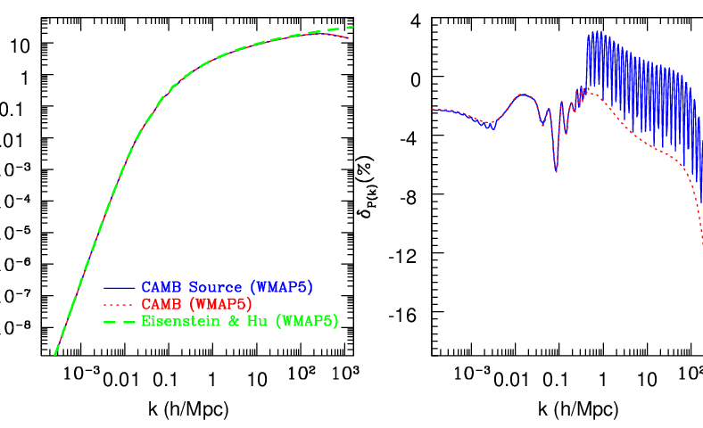
Comparing the linear power spectra proposed in the literature is an interesting task and computing an exact power spectrum on small scales is crucial for the study of formation and evolution of haloes especially in the early universe. For the CDM power spectrum Eisenstein & Hu (1998) proposed a simple fitting function that has been widely used for its simplicity, fast speed, and easy implementation. Later, the CAMB (Lewis et al., 2000) based on the CMBFAST (Seljak & Zaldarriaga, 1996), provides a fast (but not so much fast as EH method) and error-controllable package for the power spectrum. There is a variant of CAMB, the CAMB Source, which calculates more completely the small-scale transfer function considering the baryon sound speed. Figure 18 shows the differences of the CAMB and CAMB Source from the Eisenstein & Hu’s fitting function. In the left panel shown are the WMAP 5-year power spectrum linearly extrapolated to . There seems no obvious deviation between them below . But if plotted in the differential power spectrum, we are able to notice their differences more easily. The differential power spectrum defined by are shown in the right panel of the figure. The solid curve shows the difference of CAMB Source from the EH and the dotted curve is for CAMB. In this figure, we note that the EH model estimates the matter powers within a few percent accuracy on the large scale (). And intriguingly, the CAMB slightly underestimates the small-scale power compared to the CAMB Source and can not properly recover the periodic ripples either on small scales. The difference of the power amplitude between the CAMB Source and Eisenstein & Hu is, on average, less than 4% with a maximum difference of 7% around for . But for scales of interest in this study (), the power spectrum difference between the CAMBs and the Eisenstein & Hu’s becomes significant with high value. This difference is significant when measuring the power spectrum of matter or redshifted 21-cm signals. So it is very important to use the CAMB Source for generating the initial power spectrum for the minihalo studies in the early universe.
Appendix B Setting Initial Redshifts & Its Effect on the Halo Mass Functions

The GOTPM code adopts a first-order Lagrangian perturbation scheme to generate initial conditions. It is faster and simpler than the second-order scheme (Crocce et al., 2006). But the initial conditions should be generated with much care to satisfy assumptions adopted in the scheme. Like the definition in the appendix of Kim et al. (2008), the Zel’dovich redshift () of a particle is the redshift when the displacement of a particle from its Lagrangian point is equal to the mesh spacing either in , , or direction. Prior to setting up the initial conditions, particles are located at the mesh points and linear velocities are assigned to them according to the Zel’dovich approximations from which the initial displacements are calculated. Therefore, if the displacements are greater than the mesh size, they can not reflect the mesh-size fluctuations of the Zel’dovich potentials in the first-order scheme. So the initial starting redshift should properly be less than the Zel’dovich redshifts.
There is an alternative to this definition of the Zel’dovich redshift: the redshift when the relative separation between neighboring particles is zero in one of the three dimensions. This type of the Zel’dovich redshift would be the proper one if one wants to avoid the situation when two adjacent particles overshoot each other in the initial conditions. This constraint on the starting redshift would be more stringent than the original one. We call this the particle-particle Zel’dovich redshift () and the former one is renamed the particle-mesh Zel’dovich redshift (). In Figure 19, we show the distributions of (left) and (right) for simulation resolutions expressed in terms of the mean particle separation (). In the simulations we use particles and the same number of mesh to measure the initial displacement from the generated Zel’dovich potential. Therefore, one should note the lack of large-scale power in these “gauge” tests and the underestimation of the Zel’dovich redshifts are expected especially for the small cases. For the distribution, all distributions show an almost same shape with a single peak around which a power-law rising and a sharp cut off with are shown. And the distribution has double peaks with drops at higher redshifts than .

One of the easiest and simplest ways to justify the selection of the initial redshift is to measure the abundance of simulated haloes at later epochs. Simulations starting with redshifts equal to or higher than a certain critical epoch should show the same halo mass functions, and simulations with lower starting redshifts may have deviations from the true distribution. Figure 20 emphasizes the importance of in determination of the initial redshift. For simulations with cubic boxes of side length, and -size mesh, we select three chracteristic initial redshifts for comparison. First, and are chosen from distributions of and , respectively. And then, is added to contrast the lower starting redshift against above higher values. As can be seen in Figure 19, most of initial particles at are shifted larger than the mesh spacing. Using these initial settings, we run the simulations down to . The numbers of time steps are determined to satisfy that the maximum displacement of particles in a step be less than which is also set equal to the force resolution. The total time steps from to are set nearly same (ranging from 1,063 for to 1,214 for simulation) in the three simulations. It is interesting to note that at and 20 the simulation with has underpopulations of haloes ( 50%) compared to other simulations while the abundance differences narrows to a few percent level at . There is no obvious difference between the and simulations so we conclude that it would be better to use the distribution for the starting redshift of simulations.