Momentum resolved tunneling into the Pfaffian and anti-Pfaffian edges
Abstract
We calculate the electron spectral functions at the edges of the Moore-Read Pfaffian and anti-Pfaffian fractional quantum Hall states, in the clean limit. We show that their qualitative differences can be probed using momentum resolved tunneling, thus providing a method to unambiguously distinguish which one is realized in the fractional quantum Hall state observed at filling factor . We further argue that edge reconstruction, which may be less important in the first excited Landau level (LL) than in the lowest LL, can also be detected this way if present.
Introduction. Fractional quantum Hall (FQH) systems represent one of the richest and most fascinating classes of interacting electron systems known to-date. Possible realizations may include states supporting non-abelian statistics, which have been proposed to allow fault-tolerant “topological” quantum computing[1, 2]. However, in general the striking transport properties that gave the FQH effect its name are not sufficient to discriminate between various classes of different states that may occur at a given Landau level (LL) filling factor . The most hopeful experimental candidate system for a non-abelian state is the FQH state at [3]. Possible non-abelian states explaining the plateau include the Moore-Read “Pfaffian” (Pf)[4] and its particle-hole conjugate counterpart, the “anti-Pfaffian” (AP) [5, 6]. These two states have very closely related bulk properties and most fundamentally differ through the physics of their edge states. Recent experiments involving quasi-particle tunneling between opposite edges across constrictions (or point contacts) have probed quasi-particle charge[7, 8], and may have revealed signatures of non-abelian statistics[9]. They do not, however, allow for a clear distinction between the Pf and AP states; in fact only the experiment in Ref. 8 is sensitive to the difference between these two states, which shows up as a quantitative difference in certain power-law exponents. In this paper we show that momentum resolved electron tunneling (MRT) through a clean and extended junction [10, 11, 12, 13] into the edge of the state gives rise to qualitative differences in the signals, and may thus be the most promising diagnostic tool to distinguish these two states from one another, as well as from other possible states.
Experimental setup and physical assumptions.
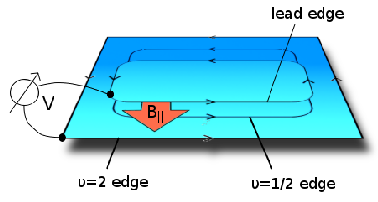
A possible experimental setup is depicted in Fig. (1), which is currently being pursued experimentally[14]. The tunneling is between the edge in the second LL and the edge of a Hall droplet in a vertically separated layer, which we assume to be in a state. We will consider both co- and counter-propagation lead geometries, i.e. the edge state propagates along the same or the opposite direction compared to that of the edge state. Note that the edge of the second LL will be contained well inside the edge of the filled lowest LL of the droplet (see Fig. (1)). While this may complicate tunneling into this edge with other settings, in that of Fig. (1) this problem is circumvented by positioning a narrow strip on top of the edge. This allows tunneling into both a co-propagating as well as a counter-propagating edge (see caption).
The Pfaffian edge theory consists of the sum of a massless chiral fermion and massless chiral boson Lagrangian density with co-propagating velocities, , where
| (1a) | ||||
| (1b) | ||||
and and are the neutral and the charged mode velocities, respectively. Here, is expected due to the fact that is associated with the larger Coulomb energy scale, in agreement with the numerics of Refs. 15, 16. In presenting the theory of the AP edge, we will follow Ref. 5, with the essential difference that we assume disorder to be so weak that momentum remains a good quantum number at the length and energy scales relevant to the experiment, and do not include it. On the other hand, disorder has been a key ingredient leading to the conclusion of universal scaling dimensions in Ref. 5. Here we will argue that the same universal exponents are also obtained, to very good approximation, based on the separation of energy scales between charged and neutral modes. In the spirit of Refs. 5, 6, we thus write the theory of the AP edge as the sum of the Pfaffian edge Lagrangian with all mode velocities reversed and that of a edge, together with a density-density interaction between the two charge modes:
| (2) |
Here, the field describes the edge, and denotes the Pfaffian Lagrangian discussed above with the formal substitution . In Eq. (2), the velocity parameters and the interaction are independent, but their relative orders of magnitude are set by the dominance of the Coulomb energy scale, as will become apparent shortly below. To see this, we carry out the charge/neutral decomposition of Ref.[5] via , . The physical significance of is that is the total charge density at the edge, while is the linear combination of and that commutes with . In terms of the new fields,
| (3) |
where , and are
simple linear combinations of , and .
In Eq. (3), however, the large Coulomb energy scale should
enter only the coupling of the total charge density
with itself, i.e. . All other coupling constants
are independent of this energy scale, and are expected to be
much smaller, i.e. .
Under these circumstances, the inter-mode coupling constant
has a very small effect of order
on the scaling dimensions of operators.
To a good approximation, we may thus set ,
which allows us to read the scaling dimensions of various
operators directly off of Eq. (3). Here we are only interested
in the most relevant operators that have the quantum numbers
of the electron operator. These operators and their scaling
dimension are then identical to those identified in
Refs.5, 6. We emphasize, however,
that the
argument given here relies on the dominance of Coulomb interactions
only and does not invoke disorder, which played
a central role in Ref. 5.
As a result, the edge theory Eq. (3) retains two distinct
counter-propagating neutral mode
velocities, and .
Electron operators and spectral functions.
An electron operator of minimal scaling dimension
is given by ,
for both the AP and Pf edge theory (we identify
in the latter).
In the Pf case, this is the unique leading electron operator,
whereas there are two more such operators of equal scaling dimension
in the AP case. These may be taken to be
.
The leading term in the electron operator at the AP edge is thus
a superposition of the operators , . However,
all cross-correlations between different vanish,
and the electron Green’s function is of the form
. We will discuss the contributions to the electron spectral function of these correlators separately. Their real space structure is given by
| (4) |
In the above, equals in the Pf case and in the AP case, whereas equals in the Pf case and in the AP case for , and for . From Eq. (4) one can obtain the Fourier transform of the electron Green’s function, and the spectral function . More directly, can be obtained from the convolution method detailed in Ref. 17. For each of the leading contributions shown in Eq. (4), the result is given by
| (5) |
with the Heaviside step function.


The results are plotted in Fig. (2) for both the Pf ()
and the AP case (). The
presence/lack of a counter-propagating mode is clearly visible.
This leads to different kinematic constraints on the
spectral weight. In the Pfaffian co-propagating
case, for any given we can make excitations
only within a finite range between
and .
In contrast,
in the AP case,
the presence of two mutually counter-propagating modes
relevant to each
excludes the spectral weight from
a finite range of frequencies, at each .
MRT conductance.
We calculate the tunneling current in linear response
using the theory discussed in Ref. 17:
| (6) |
Here is the lead spectral function. We take corresponding to a edge, with for the co-propagating lead geometry and for the counter-propagating lead geometry (cf. Fig. (1)), though other types of leads may be considered. is the Fermi-distribution function, where we assume zero temperature in the following. is the applied voltage, and is the change in the electron wavevector relative to the Fermi wavevector, where is the in-plane magnetic field and is an offset accounting for different Fermi wavevectors in the lead and the Pf or AP edge, and is the distance between the two layers. is expected to depend on as we will further discuss below. This may lead to additional distinctive features between the Pf and the AP case, since the total current is the superposition in the latter. From Eq. (6), it is straightforward to evaluate for various cases. We present a general result that is valid for any signs of and , and only assumes that is smaller than the “charged” velocity parameters and . We consider both and , which leads to qualitative differences in the co-propagating lead case. The general result can be glued together from three functions, defined as:
| (7) |
For each of these three expressions, we define an associated interval
in .
Let be the interval between and ,
the interval between and either
or , whichever is closer to .
Obviously, and share a common boundary point
and are otherwise disjoint.
Eq. (7) was written down with the tacit understanding
that the expressions for and are only valid when
, and that for is only valid for .
Outside these intervals, the associated currents are defined to be zero.
For and with these conventions, we find
for and otherwise.
The case is obtained via .
Results and discussion.
Fig. (3) shows our results for for six cases of interest,
corresponding to the Pf and AP edge state, for co- and counter-propagating
lead geometry, and for both signs of in the former case.
The most striking difference between the Pf and the AP case is apparent in the co-propagating lead geometry. Here, a positive requires a positive for a current to flow in the Pf case. In contrast, a current will always flow for a range of positive and negative values of in the AP case.
These observations are direct consequences of the kinematic constraints on
the spectral function discussed above.
Furthermore, it is only in the Pf co-propagating cases that becomes negative.
However,
even for a counter-propagating lead, the Pf and the AP case are clearly
distinguishable.
The smallest mode velocity which is visible in the graph can always
be identified with , and its sign distinguishes the Pf from the AP
case.
Also note that in Fig. 3f) (AP, counter-propagating), has no discontinuity within the region of non-zero current, but does so at one of its boundaries. In contrast, the case in Fig. 3e) (Pf, counter-propagating) shows a discontinuity within the region of non-zero current, but not at its boundaries. Furthermore, even in the AP counter-propagating case (Fig. 3f) a discontinuity in will clearly distinguish between two different regions (corresponding to and ). The separating line between these two regions has a slope, , that differs in sign from the slope of a similar separating line in the Pf counter-propagating case (Fig. 3e)).
More generally,
Figs. 3b),c),f) have no discontinuity in within the region of non-zero current, but have a discontinuity at one its boundaries, in contrast to the cases in Figs. 3a),d),e).
Note that in Fig. 3b) (Pf, co-propagating, ), smoothly goes through zero within the region where .
In any case, discontinuities in either or allow for a direct measurement of the edge mode velocities.
These findings imply that under all circumstances considered here, the MRT conductance clearly distinguishes the PF edge from the AP edge. This becomes even more pronounced when one takes into account that in the AP case, the MRT current is a superposition of the form
. For, as discussed above, the contributions do not all feature the same neutral mode velocity in the clean case considered here. Even more importantly, the offset
entering the definition of
is expected to depend on as well.
This is so because the three operators will in general carry different momenta.
To see this, we may reinterpret these operators in terms of processes taking place at the original edge and particle-hole conjugated Pfaffian edge present in Eq. (2). It is easy to see that, e.g., creates one electron at the edge while destroying two electrons at the edge. Similarly, simply destroys one electron at the edge. Hence, if different Fermi momenta are associated with the and components of the edge, all three operators carry different momenta. In the AP case, one thus expects to measure an MRT conductance which is the superposition of three graphs taken from the appropriate row in the second column of Fig. (3), with three different horizontal offsets and with two different neutral mode velocities .
We remark that the above results could in principle be affected by edge reconstruction. However, we expect these effects to be considerably weaker
at the second LL edge of interest here. Since this edge is well contained inside
the physical edge of the sample,
fringe field effects, which are usually associated with
edge reconstruction[16], will be weak.
Hence we argue that a picture based
on an unreconstructed edge may apply.
If edge reconstruction indeed occurs, additional edge modes will result and they can in principle also be detected using the setup discussed here; see Ref. 17 for a discussion of this point in the (simpler) context of a edge, and a detailed study will be left for future work (see also Ref. 18). We note that we have considered the setup of Fig. 1 both for its simplicity and experimental relevance[14]; in principle other setups like those of Refs. 10, 11, 12, 13 can also be used to study the 5/2 edge.
Finally, we mention a recent alternative proposal to distinguish
the Pf edge from the non-equilibrated AP edge, involving simple two-terminal
measurements [19]. We caution, however, that the presence of the contacts in such experiments will almost certainly lead to disorder and equilibration among the edge channels, at least near the contacts. As a result the predicted two-terminal conductance for a scenario based on non-equilibrated edges may never be observed. On the other hand, the (momentum conserving) tunneling
processes we consider occur away from these contacts, and thus do not suffer from the contact-induced disorder. We are thus hopeful that MRT will prove a useful tool to shed further
light on the
quantum Hall state in the future.
Acknowledgements.
We are indebted to M. Grayson, W. Kang, C. Nayak, and A. Yacoby for insightful discussions. This work was supported by NSF grant No. DMR-0907793 (AS), and NSF grant No. DMR-0704133 (KY).References
- [1] A. Y. Kitaev, Ann. Phys. 303, 2 (2003).
- [2] S. Das Sarma, M. Freedman, and C. Nayak, Phys. Rev. Lett. 94, 166802 (2005).
- [3] R. Willett, J. P. Eisenstein, H. L. Störmer, D. C. Tsui, A. C. Gossard, and J. H. English, Phys. Rev. Lett. 59, 1776 (1987).
- [4] G. Moore and N. Read, Nucl. Phys. B 360, 362 (1991).
- [5] S.-S. Lee, S. Ryu, C. Nayak, and M. P. A. Fisher, Physical Review Letters 99, 236807 (2007).
- [6] M. Levin, B. I. Halperin, and B. Rosenow, Physical Review Letters 99, 236806 (2007).
- [7] M. Dolev, M. Heiblum, V. Umansky, A. Stern, and D. Mahalu, Nature 452, 829 (2008).
- [8] I. P. Radu, J. B. Miller, C. M. Marcus, M. A. Kastner, L. N. Pfeiffer, and K. W. West, Science 320, 899 (2008).
- [9] R. L. Willett, L. N. Pfeiffer, and K. W. West, arXiv:0807.0221 (????).
- [10] W. Kang, H. L. Stormer, L. N. Pfeiffer, K. W. Baldwin, and K. W. West, Nature 403, 59 (2000).
- [11] I. Yang, W. Kang, K. W. Baldwin, L. N. Pfeiffer, and K. W. West, Phys. Rev. Lett. 92, 056802 (2004).
- [12] M. Huber, M. Grayson, D. Schuh, M. Bichler, W. Biberacher, W. Wegscheider, and G. Abstreiter, Physica E 22, 164 (2004).
- [13] M. Huber, M. Grayson, M. Rother, W. Biberacher, W. Wegscheider, and G. Abstreiter, Phys. Rev. Lett. 94, 016805 (2005).
- [14] A. Yacoby, private communication.
- [15] X. Wan, K. Yang, and E. H. Rezayi, Physical Review Letters 97, 256804 (pages 4) (2006).
- [16] X. Wan, Z.-X. Hu, E. H. Rezayi, and K. Yang, Physical Review B (Condensed Matter and Materials Physics) 77, 165316 (pages 15) (2008).
- [17] A. Melikidze and K. Yang, Phys. Rev. B 70, 161312(R) (2004a), Int. J. Mod. Phys. B 18, 3521 (2004b).
- [18] B. Overbosch and X.-G. Wen, arXiv:0804.2087.
- [19] C. Wang and D. E. Feldman, arXiv:0909.3111.