On P vs. NP, Geometric Complexity Theory, and the Riemann Hypothesis
Abstract
Geometric complexity theory (GCT) is an approach to the vs. and related problems suggested in a series of articles we call GCTlocal [27], GCT1-8 [30]-[35], and GCTflip [28]. A high level overview of this research plan and the results obtained so far was presented in a series of three lectures in the Institute of Advanced study, Princeton, Feb 9-11, 2009. This article contains the material covered in those lectures after some revision, and gives a mathematical overview of GCT. No background in algebraic geometry, representation theory or quantum groups is assumed. For those who are interested in a short mathematical overview, the first lecture (chapter) of this article gives this. The video lectures for this series are available at:
http://video.ias.edu/csdm/pvsnp
They may be a helpful supplement to this article.
Introduction
This article gives a mathematical overview of geometric complexity theory (GCT), an approach towards the fundamental lower bound problems in complexity theory, such as (Figure 1):
(2) The vs. problem [43]: show that .
(3) The vs. problem: show that .
We focus here on only the nonuniform versions of the above problems in characteristic zero; i.e., when the underlying field of computation is of characteristic zero, say or –what this means will be explained below. The additional problems that need to be addressed when the underlying field of computation is finite would be discussed in GCT11.
The nonuniform characteristic zero version of the conjecture (in fact, something stronger) was already proved in GCTlocal. We shall refer to it as the result without bit operations. It says that the max flow problem cannot be solved in the PRAM model without bit operations in time using processors where is the bitlength of the input. This may be considered to be the first unconditional lower bound result of GCT, because, though it can be stated in purely elementary combinatorial terms, being a formal implication of the conjecture, its proof is intrinsically geometric, and no elementary proof is known so far. Furthermore, its proof technique may be considered to be a weaker (local) form of the flip, the basic guiding strategy of GCT, which was refined and formalized much later in GCTflip. This was the begining of this geometric approach in complexity theory. The later work in GCT– the subject of this overview–focusses on the other two problems above, namely the vs. and vs. problems.
The nonuniform (characteristic zero) version of the vs. problem is also known as the permanent vs. determinant problem [43]. It is to show that , the permanent of an variable matrix , cannot be represented linearly as , the determinant of an matrix , if , or more generally, , for a fixed constant , and . By linear representation, we mean the entries of are (possibly nonhomogeneous) linear functions of the entries of . There is an analogous characteristic zero version of the vs. problem defined in GCT1, where the role of the permanent is played by an appropriate (co)-NP complete function and the role of the determinant is played by an appropriate -complete function. The main results of GCT for the vs. problem in characteristic zero also extend to the vs. problem in characteristic zero. But here we concentrate on only the former problem, since this illustrates all the basic ideas.
The complementary article [29] gives a complexity-theoretic overview of GCT. It describes the main complexity theoretic barrier towards these problems called the complexity barrier and the defining strategy of GCT for crossing it called the flip [GCT6,GCTflip]: which is to go for explicit proofs. By an explicit proof we mean a proof that provides proof certificates of hardness for the hard function under consideration that are short (of polynomial size) and easy to verify (in polynomial time). This barrier turns out to be extremely formidable and is the root cause of all difficulties in these problems. Nonelementary techniques are brought into GCT precisely to cross this barrier. It is not discussed in these lectures. The goal here is to describe the basic ideas of GCT at a concrete mathematical level without getting into such meta issues. But the readers who wish to know the need for the nonelementary techniques in GCT before getting into any mathematics may wish to read that article before this one. On the other hand, the readers who would rather avoid meta issues before getting a concrete mathematical picture may wish to read this article first. We leave the choice to the readers.
The original IAS lectures stated a lower bound called a weak form of the vs. problem. This is a special case of a more general result which we shall call a mathematical form of the conjecture (Section 1.2). It follows easily from basic results in geometric invariant theory. The article [3] showed that the weak form stated in the IAS lectures is too weak because it has a direct elementary (linear algebraic) proof. Hence in this article it has been replaced with the mathematical form of the conjecture mentioned above; cf. Section 1.2. We cannot prove this mathematical form by elementary linear algebraic proof.
The rest of this article is organized in the form of three chapters, one per lecture. The first gives a short mathematical overview of the basic plan of GCT, which is elaborated in the next two lectures.
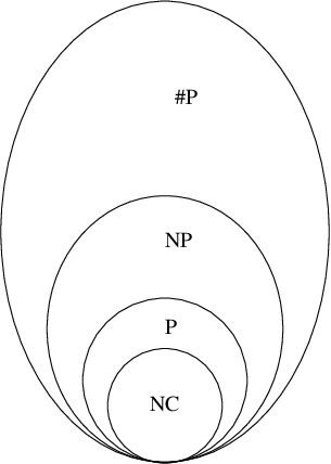
Chapter 1 Basic plan
We now outline the basic plan of GCT focussing on the permanent vs. determinant problem in characteristic zero.
1.1 Characterization by symmetries
We begin by observing that the permanent and the determinant are exceptional polynomial functions. By exceptional we mean that they are completely characterized by the symmetries in the following sense.
Let be a variable matrix. Let be the space of homogeneous forms of degree in the variable entries of . Then, by the classical representation theory, is the only form in such that, for any with ,
(D): ,
where or . Thus is completely characterized by its symmetries, and hence, is exceptional. We shall refer to this characteristic property of the determinant as property (D) henceforth.
Similarly, is the only form in the space of forms of degree in the entries of such that, for any diagonal or permutation matrices ,
(P): ,
where or with obvious constraints on the product of the diagonal entries of and when they are diagonal. Thus is also completely characterized by its symmetries, and hence, is exceptional. We shall refer to this characteristic property of the permanent as property (P) henceforth.
A basic idea [GCT1] is to a get a handle on the permanent vs. determinant problem by exploiting exceptional nature of these polynomials–i.e., their characteristic properties (P) and (D). Representation theory and algebraic geometry enter inevitably into the study of these properties, because to understand symmetries representation theory (of groups of symmetries) becomes indispensible, and to understand deeper properties of representations algebraic geometry becomes indispensible.
1.2 A mathematical form of the conjecture
To show how these characteristic properties can be exploited, we now state one application of GCT in the form of a concrete lower bound result–namely a mathematical form of the conjecture (Theorem 1.2.4 below)–before going any further.
We begin by observing that the permanent vs. determinant conjecture clearly implies that of any variable matrix can not be represented as an -computable polynomial in the traces of , , for any (possibly singular) matrices and , since can be computed fast in parallel. This can be proved unconditionally. In fact, something stronger.
Proposition 1.2.1
There do not exist (possibly singular) complex matrices and and a polynomial such that , where .
This was referred to as the weak form of the vs. problem in the original IAS lecture. The article [3] showed that this is too weak by giving an elementary linear algebraic proof [3].
We now state a more general lower bound, which was not stated in the IAS lecture, and which does not have such an elementary linear algebraic proof. For that we need a definition.
Definition 1.2.2
A polynomial function (of any degree) in the entries of variable matrices is called a generalized permanent if it has exactly the same symmetries as that of the permanent; i.e., for all nonsingular matrices and , ,
A precise description of the symmetries of the permanent is given by the property (P). Hence, and above have to be permutation or diagonal matrices (with obvious constraints on the product of their diagonal entries), or product of such matrices. When and is arbitrary, there is just one generalized permanent of degree , namely the usual permanent itself. At the other extreme, when and is arbitrary, every function in variables is a generalized permanent. For general and , almost any polynomial in ’s, , is a generalized permanent, but there are many others besides these. For general degrees, the dimension of the space spanned by generalized permanents can be exponential in ; cf. Section 3.2. In general, the space of generalized permanents has a highly nontrivial structure that is intimately linked to some fundamental problems of representation theory; cf. Section 3.2 and [GCT6].
Now we have the following:
Observation 1.2.3 (Implication of the nonuniform conjecture)
Assuming the nonuniform conjecture in characteristic zero, no -complete generalized permanent of degree can be expressed as an -computable polynomial function of the traces of , , , where , , for any complex (possibly singular) matrices and .
(Here are clearly -computable).
When and is arbitrary, this implication is equivalent to the original nonuniform conjecture (in characteristic zero), since then any polynomial in is a generalized permanent, and a polynomial function of the traces of ’s means any polynomial in . This, i.e., the general conjecture in characteristic zero, cannot be proved unconditionally at present. But the next case of this implication, and arbitrary, can be:
Theorem 1.2.4
(A mathematical form of the conjecture)
The implication above holds unconditionally for any and arbitrary .
In fact, something stronger then holds. Namely, when and is arbitrary, no generalized permanent can be expressed as a polynomial function of the traces of , , , where , , for any complex (possibly singular) matrices and .
When and is the usual permanent, this specializes to Proposition 1.2.1.
We are calling this a mathematical form for two reasons. First, it needs no restriction on the computational complexity of or the polynomial in the traces, (though for trivial reasons we can assume without loss of generality that the polynomial in the traces is computable in time, where is the degree of ). Thus it is rather in the spirit of the classical result of Galois theory which says that a polynomial whose Galois group is not solvable cannot be solved by any number of radical operations, without any restriction on the number of such operations (though again there is a trivial upper bound on the number of such operations needed if the polynomial is solvable by radicals). Second, observe that the permanent has two characteristic properties: 1) the property P (mathematical), and 2) -completeness (complexity-theoretic). The usual complexity theoretic form of the conjecture is a lower bound for all polynomial functions with the -completeness property, whereas the mathematical form is a lower bound for all polynomial functions with the property (P). In other words, the complexity theoretic form is associated with the -completeness property of the permanent and the mathematical form with the mathematical property (P).
The result indicates that there is thus a chasm between the two adjacent cases: , arbitrary (the usual nonuniform complexity theoretic conjecture), and , arbitrary (its mathematical form above). The complexity theoretic form is far far harder than the mathematical form.
For some specific generalized permanents (cf. Section 3.2), this result again has an elementary linear algebraic proof as in [3]. It also has an elementary linear algebraic proof for a generic generalized permanent. A more nontrivial part of this result (which does not have a linear algebraic proof) is that it holds for any generalized permanent. Indeed the basic difference between the complexity theoretic and the mathematical settings is the following. The complexity theoretic (i.e. the usual) conjecture is complete in the sense that if it is proved for one -complete function (say the permanent), it automatically holds for all -completeness functions (because of the theory of -completeness). But there is no such completeness theory at the mathematical level. Hence, a mathematical lower bound for a specific generalized permanent, e.g., the permanent, does not say anything about all (even -complete) generalized permanents. To get similar completeness, the mathematical form of the conjecture above covers up this lack of completeness theory at the mathematical level by proving a result for all polynomial functions with property (P), not just a specific one.
Theorem 1.2.4 has two proofs through geometric invariant theory [38]. The first proof uses only basic geometric invariant theory. Basically the proof for Proposition 1.2.1 (or rather its nonhomogeneous form) in [32] works here as well; Bharat Adsul [2] has also independenly found a similar proof. But this proof is naturalizable; i.e. it cannot cross the natural proof barrier in [40] as pointed out in [32].
The second proof sketched in this article is not naturalizable and has a deeper structure that is crucial for further progress in GCT. Specifically, it uses the same proof strategy as for the general permanent vs. determinant problem and hence serves as a test case of the general proof strategy in a nontrivial special case. Hence we shall only focus on the second proof in this article.
1.3 From nonexistence to existence
The rest of this lecture outlines the GCT approach to the general permanent vs. determinant problem, and then points out the crucial steps in this plan which can be completely executed for the mathematical form of the conjecture above, but which are conjectural at present for the general (i.e. complexity theoretic) permanent vs. determinant problem.
The first step (GCT1,2) is to reduce this nonexistence problem–i.e., that there is no small linear representation of the permanent as a determinant–to an existence problem–specifically, to the problem of proving existence of a family of obstructions; cf. Figure 1.1. Here an obstruction is a proof-certificate of hardness of , an variable matrix, just as the Kurotowski minor is a proof-certificate of the nonplanarity of a graph. Specifically, it is some algebro-geometric-representation-theoretic gadget whose existence for every serves as a guarantee that cannot be represented linearly as , when , fixed, (i.e., for greater than a large enough constant depending on ).

This reduction to existence is carried out as follows (cf. lecture 2 for details).
First, we associate (GCT1) with the complexity class a family of (group-theoretic) class varieties (what this means is explained below), and with the complexity class a family of of (group-theoretic) class varieties such that: if , , can be represented linearly as , , then
| (1.1) |
Each class variety is a (projective) algebraic variety, by which we mean that it is the zero set of a system of multivariate homogeneous polynomials with coefficients in (akin to the usual curves and surfaces). It is group-theoretic in the sense that it is constructed using group-theoretic operations and the general linear group , , of invertible complex matrices acts on it, and furthermore the groups of symmetries of the permanent and the determinant, which we shall refer to as and , are embedded in this group as its subgroups in some way. Here action means moving the points of the class variety around, just as moves the points of around by the standard action via invertible linear transformations. The goal is to show that the inclusion (1.1) is impossible (obstructions are meant to ensure this); cf. Figure 1.2.

Since each class variety has a -action, the space of polynomial functions on each class variety has a representation-theoretic structure, which puts constraints on which representations of can live on that variety (i.e., in the space of polynomial functions on that variety). Informally, an obstruction is an irreducible (minimal) representation of that can live on but not on ; cf. Figure 1.2. Existence of an obstruction , for every , assuming , fixed, implies that the inclusion (1.1) is not possible, since cannot live on . Thus an obstruction blocks the inclusion (1.1).
To define an obstruction formally, we need to recall some basic representation theory. By a classical result of Weyl, the irreducible (polynomial) representations of are in one-to-one correspondence with the partitions of length at most , by which we mean integral sequences , , where is called the length of . The irreducible representation of in correspondence with is denoted by , and is called the Weyl module of indexed by . Symbolically:
Weyl also proved that every finite dimensional representation of can be decomposed into irreducible representations–i.e., can be written as a direct sum of Weyl modules. Thus Weyl modules are the basic building blocks of the representation theory of , and every finite dimensional representation of can be thought of as a complex building made out of these blocks.
Now suppose , fixed, . Suppose to the contrary that
| (1.2) |
Let denote the homogeneous coordinate ring of ; i.e., the ring of polynomial functions 11 1 Though the functions here are not functions in usual sense; but let us not worry about this on . Let be the degree--component of consisting of functions of degree . We define and similarly. Since has the action of , also has an action of ; i.e., it is a representation of . Hence, is a finite dimensional representation of . Similarly, is a representation of , and a finite dimensional representation of .
If (1.2) holds, then we get a natural map from to obtained by restricting a function on to . By basic algebraic geometry, this map is surjective and is a -homomorphism. Furthermore, it is degree-preserving. This means there is a surjective -homomorphism from to . Symbolically:
| (1.3) |
Let denote the dual of ; i.e., the set of linear maps from to . Then (1.3) implies that there is an injective -homomorphism from to . Symbolically:
| (1.4) |
Definition 1.3.1
(GCT2) An obstruction is a Weyl module that occurs as a subrepresentation in but not in , for some . We call an obstruction label, and sometimes, by abuse of notation, an obstruction as well.
A strong obstruction is a Weyl module that occurs as a subrepresentation in but does not contain a nonzero invariant (fix point) of the subgroup of the symmetries of the determinant. It can be shown [31] that a strong obstruction is an obstruction in the above sense.
Here by an invariant we mean a point in which is fixed (does not move) with respect to the action of the subgroup .
Proposition 1.3.2
(GCT2) Existence of an obstruction , for all , with , fixed, implies , , cannot be represented linearly as , .
This follows just from the definition of an obstruction, and leads to:
Goal 1.3.3
(GCT2) Prove existence of a (strong) obstruction family using the exceptional nature of and , i.e., using the properties (P) and (D) in Section 1.1.
1.4 Obstructions for the mathematical form
The following result achieves this goal for the mathematical form (Theorem 1.2.4).
Theorem 1.4.1
There exists a (strong) obstruction family for the mathematical form of the conjecture.
This implies Theorem 1.2.4. The notion of obstructions here is similar to the one in the general case.
The proof of this result based on the results of GCT1 and 2 in geometric invariant theory [38] is outlined in the third lecture. It produces a family of (strong) obstructions, with a different than in the general complexity theoretic case. Furthermore this family is strongly explicit in the sense that the specification of each has polynomial, in fact, bitlength, and can be constructed in polynomial, in fact, time (regardless of the complexity of the polynomial in the traces in the statement of Theorem 1.2.4).
1.5 Towards existence of obstructions in general via positivity
We now proceed to describe the main results of GCT for the general (complexity-theoretic) permanent vs. determinant problem in the context of Goal 1.3.3.
Towards that end, we define certain representation-theoretic stretching functions. Let denote the number of occurences (multiplicity) of the Weyl module in (i.e. , for some ) as a subrepresentation. Let denote the multiplicity of the trivial one dimensional representation (invariant) of in . In other words, is the dimension of the subspace of invariants of in . These are statistical functions associated with the class variety and the subgroup embedding . In the first case, the statistics associates with every number (stretching parameter) the multiplicity of the corresponding Weyl module in and in the second case the dimension of the subspace of invariants of the symmetries of the determinant in ; cf. Figure 1.3.

Let us call a function quasipolynomial, if there exist polynomials , , for some , such that for all nonnegative integral modulo ; here is called the period of the quasi-polynomial. Thus quasi-polynomials are hybrids of polynomial and periodic functions. We say that is an asymptotic quasipolynomial if there exist polynomials , , for some , such that for all nonnegative integral modulo for , for some nonnegative integer depending on . The minimum for which this holds is called the deviation from quasipolynomiality. Thus is a (strict) quasipolynomial when this deviation is zero.
A fundamental example of a quasi-polynomial is the Ehrhart quasi-polynomial of a polytope with rational vertices. It is defined to be the number of integer points in the dilated polytope . By the classical result of Ehrhart, it is known to be a quasi-polynomial. More generally, let be a polytope parametrized by nonnegative integral : i.e., defined by a linear system of the form:
| (1.5) |
where is an matrix, a variable -vector, and and some constant -vectors. Let be the number of integer points in . It is known to be an asymptotic quasi-polynomial. We shall call it the asymptotic Ehrhart quasi-polynomial of the parametrized polytope . In what follows, we denote a parametrized polytope by just . From the context it should be clear whether is a usual nonparametrized polytope or a parametrized polytope.
Theorem 1.5.1
(GCT6)
(a) The function is a quasi-polynomial.
(b) The function is an asymptotic quasi polynomial.
Analogous result holds for the vs. problem in characteristic zero.
The proof of Theorem 1.5.1 is based on:
- 1.
The classical work of Hilbert in invariant theory,
- 2.
- 3.

As such, this proof is highly nonconstructive. It gives no effective bound on the period –it just says that is finite.
Remark: The original IAS lecture stated a conditional form of (b), which said that is a quasi-polynomial if the singularities of the class variety are rational and normal (in some algebro-geometric sense). Recently, Shrawan Kumar [37] has shown that the singularities of are not normal if . This means need not be a quasi-polynomial and asymptotic quasi-polynomiality as in (b) is all that we can expect. This is fine as long as the singularities of are not too bad in the sense described in Remark 3 after Hypothesis 1.6.1 below.
The following hypothesis says that can be realized as the Ehrhart quasi-polynomial of a polytope, and can be realized as the asymptotic Ehrhart quasi-polynomial of a parametrized polytope.
Hypothesis 1.5.2
(PH) [Positivity Hypothesis] (GCT6)
(a) For every , there exists a parametrized polytope such that
| (1.6) |
It is also assumed here that there exists for a specification of the form (1.5), where is independent of , and and are piecewise homogeneous linear functions of .
(b) For every , there exists a (usual nonparametrized) polytope such that
| (1.7) |
It is assumed here that there exists for a specification of the form (1.5) with and where is independent of , and is is a piecewise homogeneous linear function of .
Analogous positivity hypothesis also holds for the vs. problem in characteristic zero.
If such and exist, their dimensions are guaranteed to be small by the proof of Theorem 1.5.1: specifically, the dimension is guaranteed to be bounded by a polynomial in , and the dimension of by a polynomial in (but independent of ), if the length of is (as it would be in our applications).
When PH holds, we say that and have positive convex representations. Here positivity refers to the fact that the Ehhart function is a positive expression:
where ranges over all integer points in –there are no alternating signs in this expression. Convexity refers to the convexity of the polytopes and .
But, a priori, it is not at all clear why PH should even hold. Many numerical functions in mathematics are quasi-polynomials or asymptotic quasi-polynomials (e.g., the Hilbert function 22 2 Hilbert function of a projective algebraic variety is defined to be , where is the homogeneous coordinate ring of and its degree -component. of any projective variety), but they rarely have positive convex representations. PH is expected to hold because of the exceptional nature of the determinant and the permanent. For concrete mathematical evidence and justification, see GCT6,7, and 8.
The hypothesis PH alone is not sufficient to prove the existence of obstructions. The precise statement of a sufficient condition is given in the theorem below.
Theorem 1.5.3
(GCT6) There exists a family of (strong) obstructions for the vs. problem in characteristic zero, for , fixed, , assuming,
- 1.
PH, and
- 2.
OH (Obstruction Hypothesis):
For all , there exists such that for all large enough and .
Analogous result holds for the vs. problem in characteristic zero.
Mathematical evidence and arguments in support of OH are given in GCT6. The analogous OH that arises in the context of the mathematical form of the conjecture can be proven unconditionally.
We call a polyhedral obstruction (or rather, polyhedral obstruction-label) if it satisfies OH. In this case, , for some integer is a (strong) obstruction–we just have to choose large enough so that contains an integer point. Henceforth, whenever we say obstruction, we actually mean polyhedral obstruction.
There is a fundamental difference between the nature of PH and OH. PH is a mathematical hypothesis, because there is no constraint on what should be in comparison to in its statement. In contrast, OH is a complexity theoretic hypothesis, because needs to be small in comparison to for it to hold.
1.6 The flip: Explicit construction of obstructions
In principle PH may have a nonconstructive proof (like that of Theorem 1.5.1) which only tells that such polytopes exist without explicitly constructing them. But proving OH may not be feasible unless the polytopes and in PH are given explicitly. This suggests the following strategy for proving existence of obstructions proposed in GCT6 and GCTflip.
(1) Prove the following stronger explicit form of PH, which is reasonable since the polytopes and , if they exist, are already guaranteed to be of small (polynomial) dimension:
Hypothesis 1.6.1
(PH1) (GCT6)
(a) There exists an explicit parametrized polytope as in PH (a). Explicit means:
- 1.
The polytope is specified by an explicit system of linear constraints, where the bitlength of (the description of) each constraint is . Here and in what follows, denotes the bitlength of the description of .
- 2.
The membership problem for the polytope also belongs to the complexity class . That is, given a point , whether it belongs to can also be decided in time. Furthermore, we assume that if does not belong to the polytope, then the membership algorithm also gives a hyperplane separating from the polytope in the spirit of [15].
(b) There exists a similar explicit (nonparametrized) polytope satisfying PH (b) with the polynomial bounds that depend on and the bitlength of , but not on .
Remark 1: Note the occurrence of instead of in the polynomial bounds in (a) (which implies that the bounds here become when and ), and the absence of in the polynomial bounds in (b), which means they again are when ). The reasons for this will be explained in Lecture 3 (cf. remarks before Hypothesis 3.7.5 and after Hypothesis 3.7.9).
Remark 2: In particular, PH1 implies that the functions and belong to the complexity class .
Remark 3: PH1 also implies that the deviation from quasipolynomiality of is small, specifically, , i.e., the bitlength of the deviation is polynomial. As remarked after Theorem 1.5.1, this deviation would have been zero, i.e., would have been a (strict) quasi-polynomial, if the singularities of the class variety were all normal and rational, which, as we know now, is not the case [37]. So small deviation from quasi-polynomiality implied by PH1 basically means that the deviation from rationality and normality of the singularities of the class variety is small (cf. Theorem 1.5.1). This is the basic minimum that is required by PH1.
Like PH, PH1 is also a mathematical hypothesis in the sense that it puts no constraint on what should be in comparison to . Of course, unlike PH, there is some complexity theoretic aspect to it, but it is secondary in comparison to the complexity-theoretic aspect of OH, since smallness of with respect to is the crux of the lower bound problems under consideration.
(2a) [The flip]
Let , for a fixed . Using the explicit forms of the polytopes and in PH1, show existence of an explicit family of (polyhedral) obstructions satisfying OH. We say that an obstruction (proof-certificate) is explicit if is “short” and “easy to verify”:
- 1.
Short: This means its bitlength is , regardless what is, as long as it is , for some fixed .
- 2.
Easy to verify: given and , whether is a valid polyhedral obstruction can be verified in time. In particular, this is when .
Existence of an explicit family of polyhedral obstructions is equivalent to saying that the problem of deciding existence of polyhedral obstructions for given in unary and in binary belongs to –we shall refer to this decision problem as . This definition of explicitness is quite natural since the class is a class of problems whose proof-certificates (witnesses) are short and easy to verify. As such, the flip–going for explicit obstructions–is a proof-strategy that is literally given to us on a platter by the vs. problem itself. Why it is called flip will be explained later.
It should be stressed that we are primarily interested in only proving existence of obstructions. Whether they are explicit or not does not really matter in the original statement of the problem. But we need to know the polytopes and explicitly (as in PH1) so that proving OH is feasible. But once PH1 is proved, existence of an explicit family follows automatically, as a bonus, whether we care for it or not.
To see why, let us observe that the second condition above (ease of verification) follows directly from PH1 and the polynomial time algorithm for linear programming on polytopes given by separation oracles [15]. Shortness also follows from PH1.
Thus it is as if the vs. problem is forcing us to go for explicit obstructions.
(2b) [The strong flip (optional)]
Using the explicit forms of the polytopes and in PH1, construct (rather than just show existence of) a strongly explicit family of obstructions satisfying OH. We say that an explicit family of obstructions is strongly explicit if, for each , a valid obstruction-label can be constructed in time. In particular, the height and the bitlength of is (short) regardless what is, as long as it is , for some fixed .
For the purposes of the lower bound problems that we are interested in, the flip (just explicit existence) would suffice and the stronger flip (explicit construction) is optional. But the stronger flip can give us deeper insight into these lower bound problems; cf. [29] and GCTflip for more on this.
Now we turn to a few obvious questions.
1.7 What has been achieved by all this?: The meaning of the flip
Let us now see what has been achieved so far in the context of the conjecture in the nonuniform setting (characteristic zero), the argument for the vs. problem in characteristic zero being similar. At first glance, it may seem that all that GCT has achieved is to exchange a known difficult problem of complexity theory with a new very difficult problem of algebraic geometry. In order to see that something is gained in exchange let us reexamine the original question.
The goal of the original conjecture is to prove that , , cannot be computed by an arithmetic circuit of size , or more generally, , for some fixed , and depth . Symbolically, let denote the function computed by . Then we want to prove that
| (1.8) |
where is a sufficiently large constant and ranges over circuits of size . For given and , the problem of deciding if belongs to . Let denote the decision problem of deciding for given and (in unary) whether (1.8) holds with ranging over circuits of size . Since there are two alternating layers of quantifiers in (1.8), it belongs to , which is very high in the complexity hierarchy (cf. Figure 1.5). Hence, we refer to the original hypothesis (1.8) to be proven as IOH (Infeasible Obstruction Hypothesis). Of course, IOH is expected to be a tautology, and hence (1.8) is expected to be verifiable for small in time–but we do not know that as yet.
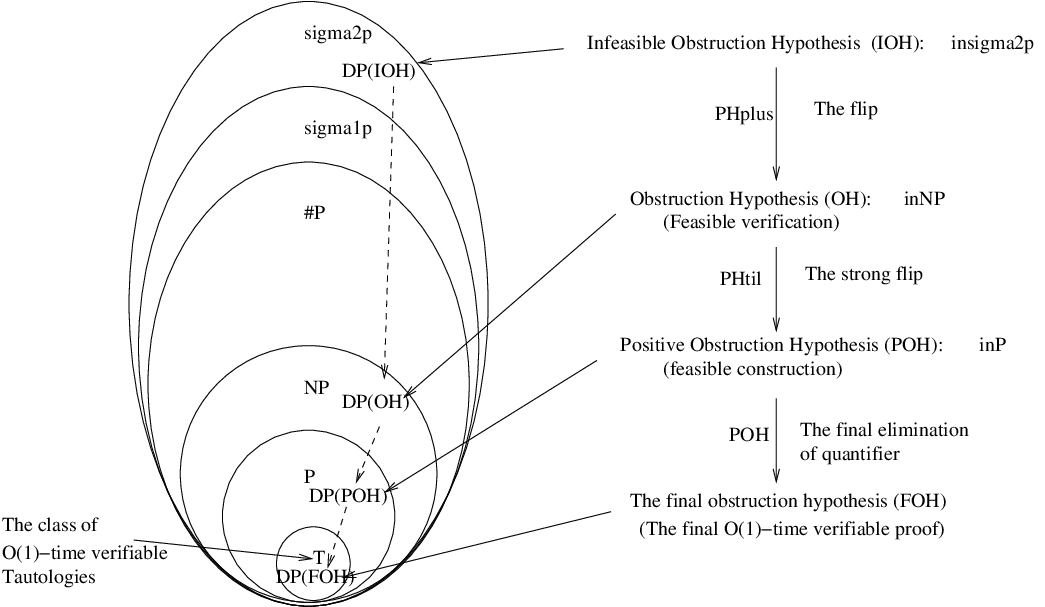
Equivalently, the goal of IOH is to prove existence of a trivial obstruction, which is a table that lists for each small as above a counterexample so that ; cf. Figure 1.6. The number of rows of this table is equal to the number of circuits ’s of size and depth . Thus the size of this table is exponential; i.e., . (Well, only if the underlying field of computation is finite. For infinite fields, such as or in this paper, there is another notion of a trivial obstruction (cf. GCT6). But let us imagine that the underlying field is finite for this argument.) The time to verify whether a given table is a trivial obstruction is also exponential, and so also the time to decide if such a table exists and construct one (optional) for given and . From the complexity theoretic viewpoint, this is an infeasible (inefficient) task. That is why we call this trivial, brute force strategy of proving IOH, based on existence of trivial obstructions, an infeasible strategy.

In contrast, assuming PH1, , the decision problem of deciding if a new polyhedral obstruction exists, belongs to (in a stronger sense assuming that is given in unary but is given in binary instead of unary) as we have already observed. Thus, assuming PH1, we have transformed the original decision problem for trivial obstructions to the decision problem for the new polyhedral obstructions , in the process bringing down the time to verify an obstruction from exponential (for the original trivial obstruction) to polynomial (for the new polyhedral obstruction); cf. Figure 1.5. It is crucial here that PH1, the main tool for this reduction, is a mathematical hypothesis, not complexity-theoretic (cf. the remarks after Theorem 1.5.3 and Hypothesis 1.6.1). The task of verifying an obstruction has also been transformed from the infeasible (exponential-time) to the feasible (polynomial-time). Hence the name of this strategy: the flip, from the infeasible to the feasible. Positivity (PH1) is used in the flip as a means to eliminate the quantifying variables in IOH and bring down the complexity of the decision problem associated with the obstruction hypothesis; cf. Figure 1.5.
This process can be extended further. Assuming an additional positivity hypothesis PH4 specified below, , whose associated decision problem belongs to , can be transformed to POH (Positivity Obstruction Hypothesis), whose associated decision problem ; i.e., whether a new obstruction exists for given in unary and in binary can then be decided in polynomial time, and if so, it can also be constructed in polynomial time; cf. Figure 1.5. (The hypothesis is called PH4 instead of PH2, because PH2 and PH3 are some other positivity hypotheses in GCT6 that complement PH1). Once this final positivity hypothesis POH is proven, the obstruction hypothesis is reduced to a tautology (FOH: Final Obstruction Hypothesis), which can be verified and constructed in time–i.e., the associated decision problem is -time solvable. This would then give us the final -size proof.
Thus the basic idea of the flip is to use positivity systematically as a means to eliminate the quantifiers and reduce the complexity of the decision problem associated with the obstruction hypothesis until the obstruction hypothesis is finally reduced to an -time verifiable tautology; cf. Figure 1.5.
Now let us specify PH4 and POH. Towards that end, let be the length of . Define
| (1.9) |
Theorem 1.7.1
The sets and are convex polytopes in .
Then:
Hypothesis 1.7.2
PH4 (GCT6) The membership problems for these polytopes belong to and so also the problem of deciding if , the volume of the relative complement , is nonzero (positive); i.e. if . By polynomial time, we mean time. This is , if and .
Hypothesis 1.7.3
(POH)
For all , assuming , fixed,
for .
1.8 How to prove PH?
There is a basic prototype of PH in representation theory, which will be described in detail towards the end of Lecture 3. We shall refer to it as Plethysm PH. It says that the stretching functions akin to and associated with fundamental multiplicities in representation theory called plethysm constants also have analogous positive convex representations.
This is known for a very special case of the plethysm constant called the Littlewood-Richardson (LR) coefficient . It is defined to be the number of occurences of the Weyl module in the tensor product of and , considered as a -module by letting act on each factor of the tensor product independently. The classical Littlewood-Richardson rule, which we shall refer to as LR PH, implies that the stretching function associated with the Littlewood-Richardson coefficient has a positive convex representation.
Plethysm PH happens to be a fundamental open problem of representation theory, older than the vs. problem itself. It has been studied intensively in the last century, and is known to be formidable. And now, as explained the third lecture, it also turns out to be the heart of this approach towards the vs , the vs. problems.
A basic plan to prove Plethysm PH is given in GCT6. It is partially implemented in GCT7 and 8. See Figure 1.7 for a pictorial depiction of the plan. It strives to extend the proof of LR PH based on the theory of the standard quantum group [12, 18, 24]. There it comes out as a consequence of a (proof of a) deep positivity result [19, 24], which we shall refer to as LR PH0. It says that the tensor product of two representations of the standard quantum group has a canonical basis [18, 24] whose structure coefficients are all positive [24] polynomials (i.e., polynomials with nonnegative coefficients). The only known proof of this result is based on the Riemann Hypothesis over finite fields proved in [10], and the related works [5]. This Riemann Hypothesis over finite fields is itself a deep positivity statement in mathematics, from which LR PH can thus be deduced, as shown on the bottom row of Figure 1.7.
If one were only interested in LR PH, one does not need this powerful machinery, because it has a much simpler algebraic-combinatorial proof. But the plan to extend the proof of LR PH to Plethysm PH in GCT6,7,8 is like a huge inductive spiral. To make it work, one needs a stronger inductive hypothesis than Plethysm PH–this is precisely Plethysm PH0 (which will be described in the third lecture; cf. Hypothesis 3.9.4). Thus what is needed now is a systematic lifting of the bottom arrow in Figure 1.7 to the top, so as to complete the commutative diagram, so to speak.
Initial steps in this direction have been taken in GCT7,8. First, GCT7 constructs a nonstandard quantum group, which generalizes the notion of a standard quantum group [12], and plays the same role in the plethysm setting that the standard quantum group plays in the LR setting. Second, GCT8 gives an algorithm to construct a canonical basis for a representation of the nonstandard quantum group that is conjecturally correct and has the property Plethysm PH0, which is a generalization of LR PH0 supported by experimental evidence. Now what is needed to complete the commutative diagram in Figure 1.7 is an appropriate nonstandard extension of the Riemann hypothesis over finite fields and the related works [5, 10, 19, 24] from which Plethysm PH0 can be deduced. This–the top-right corner of the diagram–is the main open problem at the heart of this approach.
1.9 How to prove OH or POH?
We do not know, since the proof of OH and POH would really depend on the explicit forms of the polytopes that arise in PH1/PH4, and we have no idea about them at this point. GCT does suggest that proving OH/POH should be feasible “in theory”, i.e., theoretically feasible, assuming PH1/4, since then DP(OH)/DP(POH) belong to NP/P and polynomial-time is complexity theory stands for feasible “in theory”. In other words, GCT gives a reason to believe now that proving the conjecture should be theoretically feasible. Even this was always questioned in the field of complexity theory so far, because the vs. problem is a universal statement regarding all of mathematics (that says theorems cannot be proven automatically). But, as we also know by now, there is a huge gap between theory and practice–e.g., just because some problem is in does not necessarily mean that it is feasible in practice. Similarly, the actual implementation of the GCT flip via positivity is expected to be immensely difficult “in practice”, as Figure 1.7 suggests.
1.10 Is positivity necessary?
Finally, if the positivity problems are so hard, one may ask if they can not be avoided somehow. Unfortunately, there is a formidable barrier towards the vs. and related problems, called the complexity barrier [29, 28] which is universal in the sense that any approach towards these problems would have to tackle it, not just GCT. The flip, i.e., explicit construction of obstructions, is the most natural and obvious way to cross this barrier, and the natural way may well be among the most effective. The existing mathematical evidence suggests that any such natural approach to cross this barrier would have to say something deep regarding positivity (Plethysm PH/PH0) either explicitly or implicitly, even if the approach does not utter a word about algebraic geometry or representation theory. That is, Plethysm PH and PH0 may indeed be the heart of the fundamental lower bound problems in complexity theory; a detailed story and a precise meaning of the key phrase implicit would appear in the revised version of GCTflip.

Chapter 2 Class varieties and obstructions
Let us begin by restating the permanent vs. determinant problem (characteristic zero) in a form that will be convenient here. Let be an variable matrix. Let be an variable matrix, . We assume that is the, say, bottom-right minor of , and is some entry of outside , which will be used as a homogenizing variable; cf. Figure 2.1. Let denote the space of complex matrices. Suppose , fixed, and . Then the problem is to show that there does not exist a matrix such that
| (2.1) |
where, in the computation of , is thought of as an -vector after straightening it, say, columnwise, and the result is brought back to the matrix form to compute its determinant. It is easy to see that this problem is equivalent to the homogeneous restatement of the permanent vs. determinant problem in the last lecture. The best known lower bound on at present is quadratic [26].

The goal of this lecture:
Goal 2.0.1
(GCT1,2) Reduce the permanent vs. determinant problem to a problem in geometric invariant theory (GIT) so that we can then start applying the machinery of algebraic geometry and representation theory.
Specifically,
- 1.
Define the class varieties and associated with the complexity classes and .
- 2.
Define obstructions.
- 3.
Reduce the permanent vs. determinant problem to the problem of showing existence of obstructions.
For this, we need to review some basic representation theory, algebraic geometry, and geometric invariant theory. The base field throughout is .
2.1 Basic representation theory
Let be a group. By a representation of , we mean a vector space with a homomorphism from to , the space of invertible linear transformations of . It is called irreducible if it contains no nontrivial proper subrepresentation.
Definition 2.1.1
We say that is reductive if every finite dimensional 11 1 There are some technical restrictions on what types of finite dimensional representations can be considered here (e.g. rational), which we ignore here. representation of is completely reducible; i.e., can be written as a direct sum of irreducible representations.
All finite groups are reductive–a classical fact [14]. For example, let be the symmetric group on two symbols, and its standard representation (permutation of the coordinates). Then is a direct sum of two irreducible subrepresentations given by the lines and ; cf. Figure 2.2.

Weyl proved [14] that , the general linear group of invertible matrices, is reductive, so also , the special linear group of invertible matrices with determinant one.
This means every finite dimensional representation of can be written as a direct sum:
| (2.2) |
where ranges over all finite dimensional irreducible representations of and denotes the multiplicity of in . Thus the irreducible representations are the building blocks of any finite dimensional representation.
Weyl also classified these building blocks. Specifically, he showed that the (polynomial22 2 We say that a representation is polynomial if the entries of , , are polynomial functions of the entries of .) irreducible representations of are in one-to-one correspondence with the partitions (integral sequences) of length ; we denote this partition by . It can be pictorially depicted by the corresponding Young diagram consisting of boxes in the -th row (Figure 2.3). An irreducible representation of in correspondence with a partition is denoted by , and is called a Weyl module.
For example, if , i.e., when the Young diagram consists of just one row of boxes, then is simply the space of all homogeneous forms of degree in the variables with the following action of . Given and , map to
| (2.3) |
thinking of as a row vector. This construction can be generalized to arbitrary as described in Appendix.
2.2 Basic algebraic geometry
Let , the associated projective space consisting of lines in through the origin, the coordinate ring of , which can also be thought of as the homogeneous coordinate ring of . Let be the coordinates of . A projective algebraic variety in is defined to be the zero set of a set of homogeneous forms in (it is also assumed that this zero set is irreducible; i.e., cannot be written as the union of two similar nonempty zero sets). The ideal of is defined to be the space of all forms in that vanish on . The homogeneous coordinate ring of is defined to be .
2.3 Basic geometric invariant theory
Now let be a finite dimensional representation of . Then is a -module (i.e., a representation) with the action that, for any , maps to
| (2.4) |
(This is dual of the action in (2.3)). Here denotes , where is the representation map.
Definition 2.3.1
A projective variety is called a -variety if the ideal is a -submodule (i.e., a -subrepresentation) of .
This means, under the action of , the points of are moved to the points within , i.e., each induces an automorphism of ; cf. Figure 2.4.

Let be a point, and the orbit of :
| (2.5) |
The orbit closure of is:
The closure is taken in the complex topology on by adding all limit points of the orbit.

Basic fact of algebraic geometry: is a projective -variety.
The algebraic geometry of the orbit closure for general is hopeless. It can be tractable only if is exceptional.
2.4 Class varieties and obstructions
We now construct the class varieties associated with the complexity classes and as orbit closures of suitable exceptional points (the permanent and the determinant).
Let be as in the beginning of this lecture; cf. Figure 2.1. Let be the space of homogeneous forms of degree in the entries of . It is a representation of , , with the following action. Given any , map to :
Here is thought of as an -vector by straightening it, just as in (2.1).
Similarly, let be the space of forms of degree in the entries of . It is a representation of . We define an embedding by mapping any to . This also defines an embedding of in , which we denote by again.
Let . We think of it as a point in . Let . Let . Let
| (2.6) |
We call the class variety associated with , since and is -complete. It was denoted by in the previous lecture; notice that it actually depends only on , and not on (the notation was chosen to make it look symmetric like what follows). We call the class variety associated with . It was denoted by in the previous lecture. We call the base class variety associated with .

Proposition 2.4.1
(GCT1) If , an matrix, can be expressed linearly as a determinant of an matrix, , then
| (2.7) |
or equivalently,
| (2.8) |
Conversely, if , then can be approximated infinitely closely by an expression of the form , , thinking of as an -vector.
The first statement follows because is dense in , and the second because the -orbit of is dense in .
Conjecture 2.4.2
(GCT1) If , fixed, , then .
By Proposition 2.4.1, this would solve the permanent vs. determinant problem in characteristic zero.
How to prove the conjecture?
Suppose to the contrary:
| (2.9) |
Then, by basic algebraic geometry, there is a surjective homomorphism from the homogeneous coordinate ring of to the homogeneous coordinate ring of obtained by restriction (Figure 2.7). Pictorially:
| (2.10) |

Furthermore, since the surjection is degree preserving, we get a similar surjection among the degree- components:
| (2.11) |
Since and are -varieties, these are (finite-dimensional) -modules. Furthermore, the homomorphism is a -homomorphism, again by basic algebraic geometry. By dualizing, we get an injective -homomorphism from the dual of to that of :
| (2.12) |
Definition 2.4.3
(GCT2) A Weyl module is called an obstruction for the inclusion (2.9), or an obstruction for the pair , if occurs as a -submodule in but not in , for some . We call an obstruction label, and sometimes, simply an obstruction as well.
Here occurs means the multiplicity of in is nonzero (cf. eq. (2.2)).
2.5 Why should obstructions exist?
But, a priori, it is not at all clear why such obstructions should even exist. They are expected to exist only because the class varieties , , and are exceptional, since and are exceptional (cf. Section 1.1). Next, we wish to describe in what sense the class varieties are exceptional.
2.5.1 Exceptional orbit closures (group-theoretic varieties)
For that, we need to introduce the general notion of exceptional orbit closures.
Let be any finite dimensional representation of , a point, and any nonzero point on the line in corresponding to . Let be the stabilizer of :
Definition 2.5.1
(GCT1) We say that is characterized by its stabilizer if is the only point (fix point) in such that for all .
Observation 2.5.2
If is completely characterized by its stabilizer then the orbit closure is completely determined by the associated group triple:
| (2.13) |
where the second arrow corresponds to the representation of on .
Because, once we know , we know (upto dual). And once we know the embeddings and , we know , it being the only fix point of in . We call (2.13) the group-triple associated with . We also call the associated primary couple, and the associated secondary couple.
Definition 2.5.3
The orbit closure , when is completely characterized by its stabilizer, is called a group-theoretic variety.
Coming back to the class varieties:
Proposition 2.5.4
(GCT1)
(1) The determinant , , is completely characterized by its stabilizer . Hence the class variety is group-theoretic.
Similarly, , , , and , , are group-theoretic.
Proof: Based on classical invariant (representation) theory.
(1) It is known that the stabilizer of in is the subgroup generated by linear transformations of the form:
with . Ignoring this restriction, the continuous part of is essentially embedded in naturally:
It follows from classical representation theory that is the only fix point of in .
(2) The stabilizer of in is the subgroup generated by linear transformations of the form:
where and are either diagonal or permutation matrices, with obvious constraints on the the product of the diagonal entries when they are diagonal.
The discrete part of is isomporphic to , the symmetric group, embedded in naturally:
Again, by classical representation theory, is the only fix point of in .
(3) The stabilizer of in consists of linear transformations of the form , thinking of is an -vector in which the entries of its submatrix come last, preceded by the entry , and is a matrix of the form
with (upto a constant multiple), and suitably restricted. The middle here acts on , on the -part of , and the ’s in the first column on the part of . Again is the only fix point of . Q.E.D.
2.5.2 On existence of obstructions
The main point of Proposition 2.5.4 is that the information in the class varieties is completely captured by the associated group triples. Pictorially:
| (2.14) |
where denotes equivalence at the level of information; i.e., there is no-information-loss.
Furthermore, by Tannakian duality [11], (algebraic) groups are determined by their representations; pictorially:
| (2.15) |
Thus the determinant and the permanent are encoded by the associated group triples with no information loss, and the triples, in turn, are encoded by the associated representation theories again with no information loss. This means the algebraic geometry of the class varieties is, in principle, completely determined by the geometric representation theory of the associated group triples. Hence the difference between the class varieties–which is what Conjecture 2.4.2 is all about–should be reflected as a difference between the representation theories of the associated group triples. This is why obstructions, which can be thought as representation-theoretic “differences”, should exist. See GCT2 for precise mathematical results and conjectures in the Tannakian spirit supporting this intuition.
This leads to:
Conjecture 2.5.5
(GCT2) An obstruction (label) exists for all , if , fixed.
This implies Conjecture 2.4.2.
The basic plan of GCT now is:
- 1.
Understand geometric representation theory of the group triples associated with the class varieties in depth using (nonstandard) quantum groups.
- 2.
Translate this understanding to understand the algebraic geometry of the class varieties.
- 3.
Use this understanding to find obstructions as in Conjecture 2.5.5.
2.6 The flip
The following is a stronger form of Conjecture 2.5.5:
Conjecture 2.6.1
[PHflip] (cf. GCT6 and GCTflip) There exists an explicit family of obstructions (labels), if , fixed, .
Here explicit means feasible: i.e., short and easy to verify:
- 1.
Short: the bitlength of is , for some fixed , regardless of what is, as long as it is not too large as above.
- 2.
Easy to verify: The problem of verifying obstruction-labels belongs to . That is, given and , whether is a valid obstruction-label that can belong to the above family can be decided in time, again regardless of what is, as long as it is not too large.
Here one may only consider a restricted class of obstructions (labels), and the verification algorithm may only verify if the given label belongs to that restricted class in polynomial time. This is fine as long as such restricted exists for every .
The conjecture suggests the following basic strategy, called the flip (cf. GCT6, GCTflip), for proving existence of obstructions:
- 1.
Find an “easy” criterion for verifying (recognizing) an obstruction (possibly restricted). Here easy means:
- (a)
Easy in theory: polynomial-time, and
- (b)
Easy in practice: usable in the next step.
- (a)
- 2.
Use this criterion to show existence of an explicit family of obstructions.
- 3.
More strongly (optional), show how to construct an explicit for each in time; we call such a family a strongly explicit family of obstructions.
Thus the flip reduces the hard nonexistence problem to the “easy” existence problem for obstructions.
2.7 The -barrier
By divine justice, finding such “easy” criterion for verification is an extremely hard problem.
To see why, let us examine the basic decision problems that arise in the context of verification of obstructions.
Problem 2.7.1 (Basic decision problems)
(a) Given , does occur in ?
(b) Given , does occur in ?
Actually, the following relaxed forms of these would suffice for our purpose:
Problem 2.7.2 (Relaxed basic decision problems)
(a)’ Given , does , for some integer , occur in ? If so, find one such .
(b)’ Given , does , for some integer occur in ? If so, find one such .
We need efficient polynomial-time algorithms for these relaxed decision problems.
To see the main difficulty here, observe that the dimension of the ambient space is
| (2.16) |
when , and is variable matrix. Thus is the number of monomials in variables of degree (minus one actually). Furthermore, by a classical formula of Weyl [14],
| (2.17) |
Currently the best unconditional algorithms for (a), (b), (a)’, or (b)’, based on general-purpose algorithms in algebraic geometry and representation theory take space, (the size of ). This is roughly , i.e., exponential in and hence double exponential in . The time taken is exponential in space, and hence, triple exponential in .
We cannot expect much better using such general-purpose algorithms, since they all use Grobner basis algorithms, and the problem of constructing Grobner bases is EXPSPACE-complete [25]; here EXP means exponential in the dimension .
Thus to get polynomial time algorithms for (a)’ and (b)’, we have to address:
Problem 2.7.3
[The -barrier] (cf. GCT6, GCTflip)
Bring this running time down from triple exponential in to polynomial in .
This is a massive task. For general and , it is impossible–i.e., the problems (a)’ and (b)’ are hopeless–for the reasons given above. We refer to this as the GIT chaos (GIT=Geometric Invariant Theory); cf. Figure 2.8. Conjecture 2.6.1 says, against such odds, that this task should still be possible for the exceptional and that arise in GCT, and also for similar functions characterized by their symmetries that arise in the context of the vs. problem.

Thus the main question here is:
Question 2.7.4
How to cross this -barrier?
GCT6 gives a plan for crossing this barrier assuming certain mathematical positivity hypotheses. This will be the subject of the next lecture.
Chapter 3 Positivity
In this lecture, we study positivity hypotheses in mathematics in the context of the problem of showing existence of obstructions (Conjecture 2.5.5) and the -barrier (Section 2.7).
Henceforth, we let instead of and instead of . This makes no essential difference since our ambient space is , and two points in differing by a nonzero scalar correspond to the same point in . Thus everything discussed in the first two lectures goes through for this and as well. This lecture assumes more familiarity with representation theory that in the previous lectures; Appendix covers the additional concepts needed here.
3.1 On the -module structure of the homogeneous coordinate rings of the class varieties
Given , let denote any nonzero point on the line corresponding to in . Let (not ), and (not . Let and be their stabilizers.
Theorem 3.1.1
(GCT2)
(1) occurs in (i.e., in , for some ) iff it contains a -invariant (i.e, a trivial subrepresentation–a fix point).
(2) occurs in iff contains an -invariant.
This reduces some questions concerning algebraic geometry of the class varieties to those concerning representation theory of the associated group triples (cf. Observation 2.5.2 and the remarks after it)–or rather, the associated primary couples in this case–in keeping with the basic plan discussed in Section 2.5.2.
It is easy to see that is reductive (Definition 2.1.1) from its description in the proof of Proposition 2.5.4. Hence contains a -invariant iff the dual does. Thus, this theorem also holds if we replace and by and , respectively.
Proof: We will only prove (1), (2) being similar. Let denote the affine cone of . This is the union of all lines in corresponding to the points in . Thus , the homogeneous coordinate ring of , can also be thought of as the coordinate ring of .
(A) [The trivial part]: Suppose occurs in . The goal is to show that contains a -invariant.
Fix any copy of in .
Claim 3.1.2
Not all functions in can vanish at .
Suppose to the contrary. Then, since is a -module, all functions in vanish on the orbit as well. By homogeneity of the functions in , then vanish on the cone of in . But this cone is dense in , since is dense in . Thus all functions in vanish on , and hence, cannot occur in ; a contradiction. This proves the claim.
Now consider the evaluation map at :
which maps every function in to its value at . It belongs to , the dual of . It is -invariant since is fixed by . Thus , and hence , contains a nonzero -invariant. This proves (A).
(B) [The nontrivial part]: Suppose contains a -invariant. The goal is to show that it occurs in .
For this we need the notion of stability in geometric invariant theory [38], which we now recall.
Let be a finite dimensional -representation, .
Definition 3.1.3
[38] A point is called stable with respect to the -action if the orbit is closed in in the complex (equivalently, Zariski) topology on .
Example: Let , the space of complex matrices, with the adjoint action of given by:
for any and . Then it can be shown that is stable iff is diagonalizable. For example, under the action of
we have:
Thus the orbit of the nondiagonalizable contains a diagonalizable limit point, which cannot be contained in the orbit. Hence is not stable.
Most points in any representation of are stable [38]. The nontrivial problem is to show that a specific is stable. For this, there is a very useful Hilbert-Mumford-Kempf criterion of stability [38], using which can be proved:
Theorem 3.1.4
(GCT1) The point is stable with respect to the action of . That is, the orbit is closed in .
Now let us get back to (B). Since is stable, the orbit is closed in , and hence in . That is, the orbit is a closed affine subvariety of . Hence, there is a surjective -homomorphism from the coordinate ring of to the coordinate ring of .
It suffices to show that occurs in . Now , where is stabilizer of . By the algebraic form of the Peter-Weyl theorem [14], the coordinate ring of (considered as an affine variety) decomposes as a -module:
Now
the ring of -invariants in . Thus,
Therefore occurs in iff contains an -variant. Since is reductive, this is so iff contains an -invariant. Thus occurs in .
This implies (B), and proves Theorem 3.1.1.
We now wish to state a similar result for the coordinate ring , . For that, we need a few definitions. Let and be as above. Furthermore, let , where is the bottom-right submatrix of containing and in Figure 2.1. Let . Thus we have
Let , and . Let
be the closure of the orbit . Let be its homogeneous coordinate ring.
Theorem 3.1.5
(GCT2)
(a) occurs in iff the length of is at most and occurs in .
(b) If occurs in , then it contains as a subrepresentation an -module containing an -invariant, where is the stabilizer of .
(c) Conversely, if contains an -invariant, there exists a lying over such that occurs in , and hence, occurs in . Here lying over means (a) the length of is , and (b) occurs in , considered as an -module via the natural embedding .
3.2 A mathematical form of the conjecture
We now apply GCT to prove Theorem 1.4.1 stated in the first lecture. In fact, the same proof technique yields a more general result.
To state it, we need a few definitions. Let as before, and let be embedded naturally in (each factor acts on the corresponding ). Thus the representation for can also be considered to be a representation of .
Let and its stabilizer. It consists of all linear transformations of the form:
| (3.1) |
for all . Thus , embedded in naturally:
for all . Let as before, the corresponding point in , and its stabilizer; it is esentially the stabilizer described in the proof of Proposition 2.5.4.
Let be any polynomial representation of ( copies of ). Let be a point, and any nonzero point on the line corresponding to . We say that is a generalized trace-like point if is an invariant of ( copies of ); i.e., . We say it is a generalized permanent-like point if similarly . We say that it is a generalized permanent if .
As an example, let be the ring of polynomial functions in the entries of , with the natural action of (one factor acting on the left and the other on the right), the case of the more general ring being similar. Let be the subring of the invariants of ; i.e., the subring of generalized trace-like points in . It is generated by , , by (a variant of) the first fundamental theorem of invariant theory [14]. A generalized permanent in is essentially the same as a generalized permanent in Definition 1.2.2 (for ). There is a slight difference between two definitions. In Definition 1.2.2 we let and be any matrices in , whereas here we are taking them to be in . Thus as per the definition in this section is a generalized permanent-like function, but not a generalized permanent. Everything in this section holds for a generalized permanent in Definition 1.2.2 as well. In what follows, we shall assume that a generalized permanent is as defined in this section.
Let be the subring of invariants of ; i.e., the subring of generalized permanent-like functions. By the classical result of Hilbert, it is finitely generated. No finite explicit set of generators for this ring is known (unlike for the ring of generalized-trace like functions). But an explicit basis for this ring is known. It is as follows. To every magic square of weight –i.e. a matrix of nonnegative integers whose each row and column sums to –assign a basic generalized permanent-like function
where ranges over all matrices obtained by permuting the rows and/or columns of , and , the entries of , denotes the monomial associated with . This is a -computable and -complete function of and . Furthermore, the basic generalized permanent-like functions form a basis of . Not all generalized permanent-like functions are generalized permanents. For example, , when every entry of is one, is not a generalized permanent, since it has more symmetries than that of the permanent. But most generalized permanent-like functions would be generalized permanents.
Now let be any polynomial representation of , . Given any and , let , where is the representation map. Since this map is polynomial, is well defined for any . Let denote the orbit closure of with respect to the action; i.e., the closure of the orbit .
Theorem 3.2.1
Let be any generalized trace-like point in , and and any generalized permanent in . Then, for any , . More generally, does not contain .
This reduces to Theorem 1.2.4 when . The proof in [32] based on basic geometric invariant theory also works in this case. But we are more interested here in testing the general proof strategy of GCT based on obstructions in this nontrivial special case.
We now sketch the proof of Theorem 3.2.1 based on obstructions only for . The details for the general case are similar and are left to the reader. For , Theorem 3.2.1 follows from:
Theorem 3.2.2
There exists a family of obstructions in this case.
Proof: Let be any generalized permanent, and any generalized trace-like point. The class varieties are now defined with respect to the -action and the obstructions are -Weyl-modules defined similarly. Let and be the homogeneous coordinate rings of and .
It can be using shown using Kempf’s criterion of stability [38] that is stable with respect to the action–the proof of this fact is similar to the stability related proofs in GCT1. Specifically, in this setting Kempf’s criterion in a concrete form says that is stable if the standard irreducible representation of is also an irreducible representation of its subgroup , which is easy to check. The crucial point here is that this proof needs to know only about the stabilizer of and nothing else. Using stability of it then follows from the general results in GCT2 that the analogue of Theorem 3.1.1 (2) holds for this .
The stabilizer contains the stabilizer of as described in (3.1).
We need the following two facts.
(a) Any irreducible -module is of the form . By the classical Schur’s lemma it contains a -invariant iff ;. Hence, it does not contain a -invariant if .
(b) (Cf. [4]) An irreducible representation of of the form , where stands for the trivial representation of and , contains a -invariant iff is even–if , this means every is divisible by . Here denotes the size of .
Let be any even partition with . By (b) and Theorem 3.1.1 (2) (or rather its analogue in this case mentioned above), occurs in . By (a), it does not contain a -invariant. By Theorem 3.1.1 (2) again (or rather its analogue in this case), it cannot occur in . Therefore, is an obstruction. Q.E.D.
The proof above shows that any , , which contains an -invariant is an obstruction. One can show nonconstructively, i.e., without using [4], that there is such for every . This then yields a nonconstructive proof of this result (whose major part is the same as in the explicit proof). The proof based on basic geometric invariant theory as in [32] is also nonconstructive.
3.3 From the mathematical towards the general complexity theoretic form
We now discuss what is needed to lift the proof of the mathematical form of the conjecture to the general complexity theoretic form. There are two issues.
(1) There is a serious leak in Theorem 3.1.5, because there can be several lying over , and that result does not tell us exactly which one of them would occur in or , nor does it tell us which ’s occur in or , for a fixed . Such refined information can be obtained from a general positivity hypothesis (PH: Hypothesis 1.5.2) for (which was denoted by in Lecture 1). We will discuss this issue in Section 3.7.
Problem 3.3.1
(a) Does contain a -invariant?
(b) Does contain an -invariant?
These are special cases of the general subgroup restriction problem which we discuss next in the following section.
3.4 The subgroup restriction problem
Let be a reductive subgroup of , where is an explicitly given finite dimensional representation of . Symbolically:
| (3.2) |
where denotes the representation map. For example, we can have , and , the Weyl module of . Then specifies the representation map completely, and hence, we shall also use in place of in this case–called the plethysm case. Symbolically:
| (3.3) |
Given any partition , the Weyl module of of can be considered an -module via the representation map . Since is reductive, it is completely reducible as an -module:
| (3.4) |
where denotes the multiplicity of in . In the plethysm case, we also denote by , and call it the plethysm constant.
Problem 3.4.1 (Subgroup restriction problem)
(1) Given partitions and , does occur as a subrepresentation of ? That is, is positive?
(2) Find a good positive formula for akin to the usual positive formula for the permanent which does not have any alternating signs. What good and positive means would be elaborated later (cf. Hypothesis 3.6.2).
Problem 3.4.2 (Plethysm problem)
The special case of the subgroup restriction problem for the representation map (3.3), obtained by replacing by .
The two special cases that arise in the context of Problem 3.3.1 are:
(1) Let , , and , the stabilizer of ; cf. the proof of Proposition 2.5.4 for its description. If we ignore the discrete (and torus) part of the stabilizer, then the subgroup restriction problem here is for the embedding:
(2) Let , and , and the stabilizer of ; cf. the proof of Proposition 2.5.4 for its description. If we ignore the continuous part of the stabilizer, then the subgroup restriction problem here is for the embedding:
where is the symmetric group on letters.
It is a classical result of representation theory that (1) can be reduced to the plethysm problem. By [4], (2) can also be reduced to the plethysm problem. So the plethysm problem is the fundamental special case of the subgroup restriction problem that we will be interested in (though the following results also hold for the general subgroup restriction problem).
3.5 Littlewood-Richardson problem
One completely understood special case of the subgroup restriction problem is the Littlewood-Richardson (LR) problem. This arises when embedded in diagonally:
| (3.5) |
Then every irreducible representation of is of the form . Considered as an -module via the above diagonal embedding, it decomposes:
The multiplicities are called Littlewood-Richardson coefficients. Let be the associated stretching functions.
Theorem 3.5.1
- 1.
[LR PH1] There exists a polytope of with description of bitlength such that:
the number of integer points in , and
the Ehrhart quasipolynomial of . This provides a good positive formula for the Littlewood-Richardson coefficients.
- 2.
[Saturation Theorem] [22]: iff .
- 3.
(GCT3,[22]) Given , whether is nonzero (i.e. positive) can be decided in time.
Here the third statement follows from the first two by a polynomial time algorithm for linear programming [15].
3.6 Plethysm problem
Let us now focus on the plethysm problem (Problem 3.4.2). Let be the stretching function associated with the plethysm constant . Let
be the associated generating function. It was asked in [21] if it is a rational function. The following result shows something stronger:
Theorem 3.6.1
(GCT6) The stretching function is a quasi-polynomial.
This implies, in particular, that is rational by a standard result of enumerative combinatorics [42].
The proof below is motivated by Brion’s proof [9] of quasipolynomiality of the stretching functions associated with the Littlewood-Richardson coefficients (of arbitrary type).
Proof:
Let , and . Let be the subgroup of lower triangular matrices with ’s on the diagonal. Then it is known (cf. Appendix) that there is a unique (up to constant multiple) nonzero point that is stabilized by ; i.e., such that for all . The point is called the highest weight vector of . Let be the corresponding point in . Then it is known that the orbit is already closed. That is, the orbit closure (with respect to the action) is just the orbit itself. Furthermore, by Borel-Weil [14], the homogeneous coordinate ring of has the following decomposition as an -module:
| (3.6) |
where the superscript denotes the dual. We can also think of as the coordinate ring of , the affine cone of . It is known that the singularities of are rational and normal; e.g., see [41].
Remark: By normal, we mean that for each , there exists a (classical) neighbourhood of , such that is connected; where is the subvariety of consisting of all its singular points. Rational is much more difficult to define. Roughly it means the following. By Hironaka [16], all singularities of can be resolved (untangled)–cf. Figure 1.4. With each singularity of , one can associate a cohomological object that measures the difficulty of this resolution. A singularity is called rational if this cohomological object vanishes. This means the singularity is sufficiently nice.
By abuse of terminology, we say that the ring in (3.6) is normal and rational. Similarly, it can be shown that the ring
| (3.7) |
is normal and rational. (Formally, this means the singularities of the variety, or rather the scheme, which can be associated with this ring, are rational and normal.)
Let denote the ring of -invariants in :
By (3.7),
| (3.8) |
where the superscript on the right hand side again denotes the operation of taking -invariants.
By a classical result of Hilbert [39], is a finitely generated ring (since is finitely generated). Furthermore, since is normal and rational, it follows by Boutot [6] that is normal and rational (this is the crux of the argument).
Let denote the Hilbert function of , where denotes the degree- component of .
By Schur’s lemma [14],
the multiplicity of in . Hence,
By Flenner [13], is a quasi-polynomial, since is rational and normal. Thus it follows that is also a quasi-polynomial. Q.E.D.
Hypothesis 3.6.2 (Plethysm PH)
(GCT6)
There exists a polytope of with description of bitlength such that
| (3.9) |
the Ehrhart quasi-polynomial of . In particular,
| (3.10) |
the number of integer points in .
This would provide the sought good positive formula for the plethysm constant (cf. Problem 3.4.2)
Here it is assumed that the polytope is presented by a separation oracle as in [15], and the bitlength of the description of is defined to be , where is the dimension of the ambient space in which is defined by linear constraints, and the maximum bitlength of any defining constraint. Notice that the polytope here depends only on and but not on , just like the plethysm constant itself.
Theorem 3.6.3
(GCT6) Assuming Plethysm PH, whether for some can be decided in time. If so, one such can also be found in polynomial time.
Proof: By linear programming [15]. One has to just decide if is nonempty, and if so, find a vertex of and choose such that has integral coordinates. Q.E.D.
3.7 Positivity and the existence of obstructions in the general case
Now we describe how positivity can help in proving the existence of obstructions in the general case of the vs. problem.
Towards that end, first we introduce a stronger notion of obstructions. We follow the same notation as in Section 3.1. Thus as there.
Definition 3.7.1
(GCT2) A Weyl module is called a strong obstruction for the pair , if occurs in , i.e. in for some , but does not contain a nonzero -invariant.
It follows from Theorem 3.1.1 (1) that a strong obstruction is also an obstruction as per Definition 2.4.3. Furthermore, by Theorem 3.1.5, we have:
Proposition 3.7.2
A Weyl module is a strong obstruction for the pair , iff
- 1.
The length of is at most ,
- 2.
occurs in , i.e., in for some (which has to be ).
- 3.
does not contain a nonzero -invariant.
Now let denote the multiplicity of the trivial representation of in .
Theorem 3.7.3
(GCT6) The stretching function is a quasi-polynomial.
This is proved like Theorem 3.6.1; in fact, this is essentially its special case.
The following is a precise form Hypothesis 1.5.2 (b). It is essentially a special case of Plethysm PH:
Hypothesis 3.7.4 (PH)
(GCT6)
There exists a polytope of such that
| (3.11) |
for every .
Here the polytope does not depend on or its dimension , for the same reasons that the polytope in the Plethysm PH does not depend on there; cf. the remark after the Plethysm PH. Furthermore, if exists, its dimension is guaranteed to be polynomial in the length of by the proof of Theorem 3.7.3.
The following is a precise form of Hypothesis 1.6.1 (b).
Hypothesis 3.7.5
(PH1) (GCT6)
There exists an explicit polytope satisfying PH in Hypothesis 3.7.4. Here explicit means:
- 1.
The polytope is specified by an explicit system of linear constraints, each constraint of bitlength (note no dependence on ).
- 2.
The membership problem for the polytope also belongs to the complexity class . That is, given a point , whether it belongs to can also be decided in time. Furthermore, we assume that if does not belong to the polytope, then the membership algorithm also gives a hyperplane separating from the polytope in the spirit of [15].
The following addresses a relaxed form of Problem 3.3.1, which is enough for our purposes:
Theorem 3.7.6
(1) Assuming PH1 above (Hypothesis 3.7.5), whether contains a -invariant, for some , can be decided in time. By Theorem 3.1.1, this is equivalent to deciding whether occurs in for some .
(2) Assuming an analogous PH1 for the subgroup restriction problem for , whether contains an -invariant, for some , can also be decided in time. By Theorem 3.1.1, this is equivalent to deciding whether occurs in for some .
Proof: Similar to that of Theorem 3.6.3. Q.E.D.
A similar result for or would not follow from the Plethysm PH (or more generally, the subgroup restriction PH) because of the serious leak in Theorem3.1.5 that we discussed in Section 3.3. One needs a more general PH for this. We turn to this issue next.
For any of length , let be the multiplicity of in , which by Theorem 3.1.5, coincides with the multiplicity of in . Thus is the same as the function with the same notation in Theorem 1.5.1 (b). The following is its restatement.
Theorem 3.7.7
The function is an asymptotic quasi-polynomial.
The singularities of the class variety here are not normal [37] when . But in view of the exceptional nature of the class variety and Theorems 3.6.1 and 3.7.3, it may be conjectured that the deviation from rationality and normality is small; cf. the remarks after Hypothesis 3.7.9 below.
The following is a restatement of Hypothesis 1.5.2 (a).
Hypothesis 3.7.8
If such exists, its dimension is guaranteed to be polynomial in (by the proof of Theorem 3.7.7) essentially because the dimension of is and does not depend on .
The following is a restatement of Hypothesis 1.6.1 (a).
The meaning of explicit here is as in Hypothesis 1.6.1. In particular, the polynomial bounds are meant to be polynomial in and , instead of . Because is the multiplicity of in , , which does not depend on , and occurs only in the definition of as a numeric parameter akin to the numeric parameters ’s.
Furthermore, PH1 above implies that the deviation from quasipolynomiality of is small, specifically, , so that the bitlength of the deviation is polynomial. This would mean that the deviation from rationality and normality of the singularities of the class variety is also small; cf. Theorem 3.7.7 and the remarks after it.
Theorem 3.7.10
Assuming general PH1 (Hypothesis 3.7.9), whether occurs in –or equivalently, whether occurs in –for some , can be decided in time.
The following is a refined version of Theorem 1.5.3:
Theorem 3.7.11
(GCT6) There exists a family of strong obstructions for the general vs. problem in characteristic zero, for , fixed, , assuming,
- 1.
- 2.
OH (Obstruction Hypothesis):
For all , there exists such that for all sufficiently large and .
For an analogous result for the vs. problem, see GCT6.
We define to be a polyhedral obstruction (label) if it satisfies OH here. In this case it is easy to see that , for some , is a strong obstruction.
3.8 Positivity and the -barrier
Theorem 3.8.1
In conjunction with Theorem 3.7.11, this implies its stronger form:
Theorem 3.8.2
(GCT6) There exists an explicit (cf. Section 1.6) family of polyhedral obstructions, for the general vs. problem in characteristic zero, for , fixed, , assuming PH1 and OH above.
Analogous result holds for the vs. problem in characteristic zero.
The strategy now is to prove PH, or rather PH1, first, and then prove OH using the explicit forms of the polytopes in PH1. GCT2,6,7,8 together give an evidence for why PH/PH1 and OH should hold. As far as proving OH is concerned, there is nothing that we can say at this point since it depends on the explicit forms of the polytopes in PH/PH1. The remaining question is the following.
3.9 How to prove PH1 and why should it hold?
We now briefly describe the plan in GCT6 to prove PH1 by generalizing the proof of LR PH1 (Theorem 3.5.1) based on the theory of standard quantum groups [12, 18, 24].
For that we need a definition.
Definition 3.9.1
Let be a connected reductive subgroup of a connected reductive . A basis of a representation of is called positive with respect to the -action if:
- 1.
If it -compatible. This means there exists a filtration of :
such that , where denote the linear span of , is isomorphic to an irreducible -module. In other words, this filtration gives a Jordan-Holder series of .
- 2.
For each standard generator of (the Lie algebra of) and each ,
where each is a nonnegative rational.
LR PH1 is a consequence of the proof of a much deeper positivity result:
Theorem 3.9.2 (LR PH0)
The proof of this result goes via the theory of the standard quantum group. Specifically, the diagonal embedding (3.5) is first quantized [12] in the form
| (3.13) |
where is the standard quantum group, a quantization of that plays the same role in quantum mechanics that the standard group plays in classical mechanics. (Well, (3.13) is not really accurate, because what is quantized in [12] is not but rather its universal enveloping algebra. We shall ignore this technicality here.) It is then shown that the irreducible representations of and have extremely rigid canonical bases [18, 24], which are positive [24], and have many other remarkable properties. The only known proof of this positivity [24] is based on the Riemann hypothesis over finite fields and the related works [10, 5]
Goal 3.9.3
Lift this LR story to the plethysm problem (and the more general subgroup restriction problem).
In this context:
Hypothesis 3.9.4 (Plethysm PH0)
Let
| (3.14) |
be the plethysm homomorphism (3.3). The each Weyl module has a positive basis with respect to the -action.
Theorem 3.9.5
(GCT7) The plethysm map (3.14) can be quantized in the form
| (3.15) |
where is the standard quantum group associated with and is a new nonstandard quantization of .
A similar result holds for general connected reductive as well.
Furthermore, GCT8 gives a conjecturally correct algorithm to construct canonical bases of irreducible representations with conjectural positivity and other properties from which Plethysm PH0 would follow. Experimental evidence for positivity of the conjectural canonical bases in GCT8 constitutes the main evidence for Plethysm PH0, and hence Plethysm PH1/PH.
The general PH1 (Hypothesis 3.7.9) can be regarded as a generalization of the Plethysm PH1 for the triple (cf. Observation 2.5.2)
| (3.16) |
associated with the class variety , rather than the plethysm couple (3.14). To go from the Plethysm PH1 to the general PH1, one has to similarly quantize the triple (3.16) and develop an analogous theory of canonical bases for this quantized triple. But first, we have to understand the couples. Hence the Plethysm PH0/PH1 can be regarded as the heart of GCT. To prove the nonstandard quantum group conjectures in GCT7,8 that arise in this context, a substantial nonstandard extension of the work [10, 5, 19, 24] surrounding the standard Riemann hypothesis over finite fields may be necessary; cf. Figure 1.7. Thus the ultimate goal of GCT would be to deduce the ultimate negative hypothesis of mathematics, conjecture (in characteristic zero), from the ultimate positive hypotheses–namely, as yet unknown, nonstandard Riemann hypotheses (over finite fields); cf. Figure 3.1.

Bibliography
- [1] S. Aaronson, Is P versus NP formally independent? Bulletin of the EATCS 81: 109-136 (2003).
- [2] B. Adsul, private communication.
- [3] B. Alexeev, J. Tsimerman, A direct proof of Mulmuley’s weak versus result, manuscript.
- [4] S. Ariki, J. Matsuzawa, I. Terada, Representations of Weyl groups on zero weight spaces of -modules, Algebraic and topological theories, pp. 546-568 (1985).
- [5] A. Beilinson, J. Bernstein, P. Deligne, Faisceaux pervers, Astérisque 100, (1982), Soc. Math. France.
- [6] J. Boutot, Singularit’es rationelles et quotients par les groupes r’eductifs, Invent. Math.88, (1987), 65-68.
- [7] M. Brion, On the general faces of the moment polytope, IMRN International Mathematics Research Notices, No. 4, 1999.
- [8] S. Cook: The complexity of theorem-proving procedures. Proceedings of the third annual ACM Symposium on Theory of Computing. 151-158. (1971).
- [9] R. Dehy, Combinatorial results on Demazure modules, J. of Algebra 205, 505-524 (1998).
- [10] P. Deligne, La conjecture de Weil II, Publ. Math. Inst. Haut. Étud. Sci. 52, (1980) 137-252.
- [11] P. Deligne, Categories tannakiennes, in The Grothendieck Festschrift, Volume 2, 11-195, Birkhauser, 19990.
- [12] V. Drinfeld, Quantum groups, Proc. Int. Congr. Math. Berkeley, 1986, vol. 1, Amer. Math. Soc. 1988, 798-820.
- [13] H. Flenner, Rationale quasi-homogene singularitäten, Arch. Math. 36 (1981), 35-44.
- [14] W. Fulton, J. Harris, Representation theory, A first course, Springer, 1991.
- [15] M. Grötschel, L. Lovász, A. Schrijver, Geometric algorithms and combinatorial optimzation, Springer-Verlag, 1993.
- [16] H. Hironaka, Resolution of singularities of an algebraic variety over a field of characteristic zero, Ann. of Math (2), 79: 109-273.
- [17] R. Karp: Reducibility among combinatorial problems. R. E. Miller and J. W. Thatcher (eds.) Complexity of computer computations, Plenum Press, New York, 1972, 85-103.
- [18] M. Kashiwara, On crystal bases of the -analogue of universal enveloping algebras, Duke Math. J. 63 (1991), 465-516.
- [19] D. Kazhdan, G. Lusztig, Schubert varieties and Poincare duality, Proc. Symp. Pure Math., AMS, 36 (1980), 185-203.
- [20] G. Kempf: Instability in invariant theory, Annals of Mathematics, 108 (1978), 299-316.
- [21] A. Kirillov, An invitation to the generalized saturation conjecture, math. CO/0404353., 20 Apr. 2004.
- [22] A. Knutson, T. Tao, The Honeycomb model of tensor products I: proof of the saturation conjecture, J. Amer. Math. Soc, 12, 1999, pp. 1055-1090.
- [23] A. Levin: Universal sequential search problems. Problems of information transmission (translated from Problemy Peredachi Informatsii (Russian)) 9 (1973).
- [24] G. Lusztig, Canonical bases arising from quantized enveloping algebras, J. Amer. Math. Soc. 3, (1990), 447-498.
- [25] E. Mayr, and A. Meyer, The complexity of the word problems for commutative semigroups and polynomial ideals, Advances in mathematics, 46 (3): 305-329, 1982.
- [26] T. Mignon, N. Ressayre, A quadratic bound for the determinant and permanent problem, International Mathematics Research Notices (2004) 2004: 4241-4253.
- [27] K. Mulmuley: Lower bounds in a parallel model without bit operations, The SIAM Journal On Computing, vol. 28, no. 4, 1999.
- [28] K. Mulmuley, On P vs. NP, geometric complexity theory, and the flip I, Technical report TR-2007-16, computer science department, The university of Chicago, September 2007; revised version under preparation. This and the following GCT papers are available at http://ramakrishnadas.cs.uchicago.edu.
- [29] K. Mulmuley, On P vs. NP, Geometric Complexity Theory, Explicit proofs, and the Complexity Barrier, under preparation, to be available at the above website soon.
- [30] K. Mulmuley, M. Sohoni, Geometric complexity theory I: an approach to the vs. and related problems, SIAM J. Comput., vol 31, no 2, pp 496-526, 2001.
- [31] K. Mulmuley, M. Sohoni, Geometric complexity theory II: towards explicit obstructions for embeddings among class varieties, SIAM J. Comput., Vol. 38, Issue 3, June 2008.
- [32] K. Mulmuley, An appendix to Geometric Complexity Theory II, technical report, computer science department, the university of chicago, February, 2009.
- [33] K. Mulmuley, Geometric complexity theory VI: The flip, Revised version under preparation, Earlier version: Technical Report TR-2007-04, computer science department, The University of Chicago, September, 2007.
- [34] K. Mulmuley, Geometric complexity theory VII: Nonstandard quantum group for the plethysm problem, Technical Report TR-2007-14, computer science department, The University of Chicago, September, 2007.
- [35] K. Mulmuley, Geometric complexity theory VIII: On canonical bases for the nonstandard quantum groups, Technical Report TR 2007-15, computer science department, The university of Chicago, September 2007.
- [36] K. Mulmuley, Geometric complexity theory XI: on the flip over fields of positive characteristic, under preparation.
- [37] Shrawan Kumar, private communication.
- [38] D. Mumford, J. Fogarty, F. Kirwan: Geometric invariant theory. Springer-Verlag, 1994.
- [39] V. Popov, E. Vinberg, Invariant theory, in Encyclopaedia of Mathematical Sciences, Algebraic Geometry IV, Eds. A. Parshin, I. Shafarevich, Springer-Verlag, 1989.
- [40] A. Razborov, S. Rudich, Natural proofs, J. Comput. System Sci., 55 (1997), pp. 24-35.
- [41] K. Smith, F-rational rings have rational singularities, Amer. J. Math. 119 (1997).
- [42] R. Stanley, Enumerative combinatorics, vol. 1, Wadsworth and Brooks/Cole, Advanced Books and Software, 1986.
- [43] L. Valiant: The complexity of computing the permanent. Theoretical Computer Science 8 , 189-201 (1979).
Appendix: A bit more of representation theory
Here we go into the basic representation theory a bit more than in Section 2.1; in particular, we describe an explicit construction of Weyl modules.
Let be a group. We say that a vector space is a representation of , or a -module, if there is a homomorphism
| (3.17) |
where is the general linear group of invertible transformations of . We denote by –the result of the action of on . A -subrepresentation is a subspace that is invariant under ; i.e., for every . If is clear from the context, we just call it subrepresentation. We say that is irreducible if it does not contain a proper nontrivial subrepresentation. A -homomorphism from a -module to a -module is map such that for all .
We say that is reductive if every finite dimensional representation of is completely reducible. This means it can be expressed as a direct sum of irreducible representations in the form
| (3.18) |
where ranges over all indices (labels) of irreducible representations of , denotes the irreducible representation of with label , and denotes a direct sum of copies of . Here is called the multiplicity of in . It is a basic fact of representation theory that for reductive groups, the decomposition (3.18) is unique; i.e., ’s are uniquely defined. If , we say that occurs in .
An example of a nonreductive group is a solvable group that is not abelian. In this case a subrepresentation need not have a complement such that .
Every finite group is reductive. Thus , the symmetric group on letters, is reductive. A prime example of a continuous reductive group is the general linear group , the group of nonsingular matrices, and its subgroup the special linear group of matrices with determinant one. Any product of reductive groups is also reductive. These are the only kinds of reductive groups that we need to know in this article. So whenever we say reductive, the reader may wish to assume that the group is a general or special linear group or a symmetric group or a product thereof.
We say that the representation (3.17) of or is polynomial if for every , every entry in the matrix form of is a polynomial in the entries of .
Complete reducibility as in eq.(3.18) means every finite dimensional representation of a reductive group is composed of irreducible representations. These can be thought of as the building blocks in the representation theory of reductive groups, and it is important to know what these building blocks are.
For and this was done by Weyl [14]. The polynomial irreducible representations of are in one-to-one correspondence with the tuples of integers, where and . Here is called a partition of length and size . Its bitlength is defined to be the total bitlength of all ’s.
Thus the polynomial irreducible representations of are labelled by partitions of length at most , but any size. The irreducible representation corresponding to a partition is denoted by , and is called a Weyl module of . When is clear from the context, we shall denote it by simply .
Each partition corresponds to a Young diagram, which consists of rows of boxes, with boxes in the -th row. For example, the Young diagram corresponding to is shown below:
When thinking of a partition, it is helpful to think of the corresponding Young diagram. Thus each Weyl module is labelled by a Young diagram of height at most . This is a useful combinatorial tool for studying the Weyl modules.
A Weyl module is explicitly constructed as follows. This construction of Deyruts as well as Weyl’s original construction are given in [14]. Let be an variable matrix. Let be the ring of polynomials in the entries of . It is a representation of . Action of a matrix on a polynomial is given by
| (3.19) |
By a numbering (filling), we mean filling of the boxes of a Young diagram by numbers in ; for example:
We call such a numbering a (semistandard) tableau if the numbers are strictly increasing in each column and weakly increasing in all rows; e.g.
The partition corresponding to the Young diagram of a numbering is called the shape of the numbering.
With every numbering , we associate a polynomial , which is a product of minors for each column of . The minor for a column of length is formed by the first rows of and the columns indexed by the entries , , of . Thus , where ranges over all columns in . The Weyl module is the subrepresentation of spanned by , where ranges over all numberings of shape over . Its one possible basis is given by , where ranges over semistandard tableau of shape over .
Let be the subgroup of upper triangular matrices. It is called the Borel subgroup of . An element is called a highest weight vector if it is an eigenvector for the action of each . It is easy to show that has a unique highest weight vector, upto a constant multiple: it is , where is the canonical tableau whose -th row contains only ’s, for each ; e.g.
Let be the subgroup of upper block triangular matrices, where the sizes of the blocks are fixed. For example:
Such subgroups are called parabolic. Let be the (projective) stabilizer of the highest weight vector ; i.e., the set of all such that , for some complex number . Then it is easy to show that is parabolic, where the sizes of the blocks are completely determined by .
The irreducible representation of corresponding to the Young diagram that consists of just one column of length is the determinant representation: . When restricted to the subgroup this becomes trivial. More generally, and give the same representation of if is obtained from by removing columns of length . Hence, irreducible polynomial representations of are in one to one correspondence with partitions of length less than , and are obtained from the ones of by restriction.
¡