On P vs. NP, Geometric Complexity Theory, Explicit Proofs and the Complexity Barrier
Abstract
Geometric complexity theory (GCT) is an approach to the vs. and related problems. This article gives its complexity theoretic overview without assuming any background in algebraic geometry or representation theory.
1 Introduction
Geometric complexity theory (GCT) is an approach to the vs. [14, 29, 33], permanent vs. determinant [57] and related problems (Figure 1) suggested in a series of articles we call GCTlocal [36], GCT1-8 [41]-[49], and GCTflip [39]. There seems to be a fundamental root difficulty, which we call the complexity barrier, that must be overcome by any proof technique that could settle these problems. Not surprisingly this barrier turns out to be extremely formidable. All the mathematical effort in GCT in a sense goes towards crossing this barrier. In fact, even formalization of this barrier turns out to be quite nonelementary and cannot be done at present without algebraic geometry and representation theory. The main result of GCT [GCT6] provides such a formalization and a mathematical programme for crossing the barrier, which has been partially implemented in [GCT6,7,8,11]–this turns out to be quite a nonelementary affair. This paper provides an informal exposition of the complexity barrier to explain why it may be the root difficulty of the vs. problem and what makes it so formidable so that the need for these nonelementary techniques that enter into GCT to tackle this barrier becomes clear at a high level.
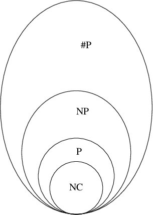
But before we turn to this barrier, let us first see why the earlier known barriers such as the relativization [7], natural-proof [55], algebraic degree [GCTlocal] and algebrization [2] barriers do not really capture the main source of difficulties that needs to be overcome by an eventual proof. This became clear after these barriers were bypassed in the early papers of GCT [GCTlocal,GCT1,GCT2]. Let us now explain how these barriers were bypassed in these early papers, and then explain why the root difficulty still remained after bypassing them.
Let us begin with [GCTlocal] that proves a special case of the conjecture called the result without bit operations. This may be considered to be the first concrete lower bound result of GCT. It was proved using a weaker form of GCT’s strategy for crossing the complexity barrier (discussed below) much before it was formalized in [GCTflip,GCT6]. The result says that the maxflow problem cannot be solved in the PRAM model without bit operations in polylogarithmic time using polynomially many processors. At present this may be the only superpolynomial lower bound that is a special case of any of the fundamental separation problems in Figure 1 and holds unconditionally in a natural and realistic model of computation that is heavily used in practice. Furthermore, as explained in Section 6, its proof technique is fundamentally different from the proof techniques to which the relativization and natural-proof barriers apply.
But that is not enough. Because GCTlocal pointed out a third barrier in complexity theory, which we shall call the algebraic degree barrier, but which was not called a barrier there for the reasons explained below. This basically says that any low degree or degree based proof technique, such as the one there, which associates with a computation algebraic objects and then reasons solely on the basis of the degrees of those objects will not work for unrestricted fundamental separation problems. As far as we can see, the recent algebrization barrier [2] also suggests something similar 11 1 But on the basis of lower bounds which may not be as closely related with the fundamental separation problems in Figure 1 as the result without bit operations in GCTlocal.. Hence it is not treated separately in this article.
GCTlocal also suggested an idea for crossing the algebraic degree barrier: namely, associate with complexity classes algebraic varieties with group actions that capture the symmetries of computation and then reason on the basis of the deeper representation theoretic structure of these varieties rather than just their degrees.
This led to the investigation in GCT1 and 2, which suggested an approach to the fundamental lower bound problems via algebraic geometry and representation theory. This approach bypasses the relativization, natural proof and algebraic degree barriers simultaneously as explained in Sections 7 and 8. In contrast, it seems [2] that the earlier known techniques for proving lower bounds in complexity theory may not bypass these well studied barriers simultaneously.
Unfortunately after GCT1 and 2, wherein the earlier known barriers were thus bypassed, it became clear that the root difficulty of the vs. problem still remained after bypassing these barriers and the main battle on the vs. problem really begins only after bypassing them.
In retrospect, this should not be surprising. The relativization, natural-proof, and algebraic-degree barriers cannot be expected to capture the root difficulty of the vs. problem.
To see why, let us begin with the algebraic degree barrier in [GCTlocal]. It applies to the low degree techniques of the kind used in that paper. All these techniques are in one way or the other related to the fundamental Bezout’s theorem in algebraic geometry and the notion of a degree of a polynomial (we also include the low degree techniques used in other areas of complexity theory in this category). Though this is a nontrivial area of mathematics, it is still very small compared to the whole of mathematics. Hence, we can say that this barrier is local in the sense that it applies to a very restricted class of techniques in mathematics. If a proof technique does not belong to this class, the barrier is simply bypassed, i.e., is not applicable. In this sense, it is not really a barrier–if by a barrier we mean a conceptual obstacle that any eventual proof of the conjecture would need to overcome regardless of which areas of mathematics it goes through–but rather a trap that a proof technique has to avoid. This is why it was not called a barrier in GCTlocal.
We can also say that the algebraic degree barrier is primarily mathematical in the sense that low degree is a purely a mathematical notion, there is no complexity theory in it, and though it is very useful in complexity theory, this barrier is really a statement about the restricted nature of these mathematical techniques rather than about the complexity theoretic difficulty of the vs. problem.
In a similar way, we may say that the relativization and natural proof barriers are also local and mathematical. Mathematical because the natural proof barrier is generally regarded as applying to proof techniques that work for most functions and most is a mathematical notion, so also the notion of relativization.
Now we can explain why local mathematical barriers cannot be expected to capture the root difficulty of the vs. problem. Because this problem is a universal complexity-theoretic statement about all of mathematics. Namely, if this conjecture fails to hold, every theorem in mathematics that has a proof of reasonable length can be proved efficiently by a computer in time polynomial in the length of its shortest proof. No other known conjecture in mathematics has such stunning mathematical sweep. Given the universal complexity theoretic nature of this problem, it then stands to reason that the main barrier towards this problem–the root cause of its difficulty–should also be universal and complexity theoretic, where by a universal barrier we mean a barrier that every approach has to cross regardless of which areas of mathematics it goes through. In other words, a local barrier is like a guiding post which tells us what must not be done, and hence must be bypassed, whereas a universal barrier cannot be bypassed no matter what, because it tells us what must be done, i.e., it has to be crossed. A local barrier only rules out a restricted area of mathematics. Regardless of how many restricted areas of mathematics we rule out in this way, that still rules out only a small subarea of mathematics, tells us a few things that we should not do, but gives us essentially no idea about what to do given that the vs. problem is a statement about all of mathematics. At some point we have to turn our attention from what is not to be done to what is to be done and identify the root universal and complexity theoretic difficulty of this problem; i.e., a universal complexity theoretic barrier.
The complexity barrier described in this article seems to be this universal complexity theoretic barrier. Crossing this barrier basically means answering formally the folklore question: why should the vs. problem not preclude its own proof by standing in the way of any approach, and hence, why should any given approach be feasible even theoretically? The key phrase here is answering formally. This means: (1) fix an appropriate proof strategy (approach) and formalize the question by defining precisely and formally what theoretically feasibility of this fixed proof strategy means, and (2) then answer the formalized question by proving that this proof strategy is indeed theoretically feasible as per this definition. In other words, formalization of the informal folklore question as in step (1) is itself a part of the challenge. If this is carried out, we say that the complexity barrier has been formalized in this approach. The conjecture seems so severe that for most proof strategies it may not even be possible to carry out step (1). That is, formal definition theoretical feasibility may be possible for only some exceptional proof strategies. This is why just formalization of the complexity barrier seems to be such a challenge.
The most obvious and natural abstract strategy to cross the complexity barrier, called the flip [GCT6,GCTflip], is suggested by the vs. problem itself. It is to go for its explicit proof. By this we mean a proof that shows existence of proof certificates of hardness for an NP-complete function that are short of size and easy to verify in time; i.e., the problem of verification of the proof certificates belongs to and hence is theoretically feasible. In other words, the flip seeks proof certificates for nonmembership of in akin to those for its membership in . Abstractly, GCT is any geometric approach to the vs. and related problems based on the flip; i.e., on construction of explicit proofs. Such explicit proofs based on the specific proof certificates defined in GCT1,2 and 6, called geometric obstructions, exist as per the explicit proof conjecture [GCT6]. The main result of GCT is a complete formalization [GCT6] of the complexity barrier (in this specific approach) and a mathematical programme [GCT6,7,8,11] to cross the formalized complexity barrier via the flip for the vs. and related problems.
This article gives a complexity theoretic overview of GCT outlining these developments.
This also allows us to place GCT in the landscape of all possible approaches to cross this main barrier in complexity theory. For that, we define GCT abstractly as any geometric approach based on the flip towards the vs. and related problems, where geometric means based on the symmetries of a judiciously chosen . The present formal GCT is one such approach. Though the flip is the most obvious and natural way to cross the complexity barrier, paradoxically it also turns out to be very counterintuitive and hard to believe at the same time. The formalization of the complexity barrier mentioned above basically provides a concrete mathematical program to implement the flip and says that the flip should be feasible however counterintuitive it may seem. The main goal of this article is to justify this from the complexity theoretic perspective. Two concrete lower bounds of GCT mentioned above play a crucial role in this justification.
The complementary article [40] gives a mathematical overview of GCT based on the IAS lectures without getting into the meta issues concerning barriers. The reader who wishes to get a concrete mathematical picture of the approach before worrying about such issues may wish to read that article first. On the other hand, the reader who wishes to know the root difficulty of the vs. and related problems and the need for nonelementary techniques before getting into any mathematics may wish to read this article first. We leave the choice to the readers. See also the recent article [12] for an external mathematical review of GCT1 and 2.
The rest of this article is organized as follows. The complexity barrier is discussed in Section 2, high level statement of the main result of GCT–a formalization of the complexity barrier–in Section 3. Abstract flip is described in Section 5, the result without bit operations in Section 6, the meaning of the phrase geometric in Section 7, why GCT bypasses the earlier known local barriers simultaneously in Section 8, elaboration of the main result in Sections 10 and 12, and finally the question–is the complexity barrier really so formidable?–in Section 13. Sections 7-12 constitute an extended abstract of Chapter 1 in [40].
Remark: Natural in GCT means explicit unlike in [55] where it means probabilistic. The meaning should be clear from the context.
Acknowledgements: The author is deeply grateful to Janos Simon without whom this paper would not exist. The paper grew out of a series of discussions on GCT with him over the last year. The goal was to communicate to him the root difficulty that GCT is trying to overcome and its basic plan for doing so. That root difficulty is the complexity barrier described here. This paper basically consists of answers to his tough and insightful questions. The author is also grateful to Scott Aaronson, Laci Babai, Josh Grochow, Russell Impagliazzo, Hari Narayanan, Partha Niyogi, Sasha Razborov, and Avi Wigderson for helpful discussions.
2 Complexity barrier
In this section we describe the complexity barrier.
Towards that end, let us fix an -complete function , say SAT. The goal of the nonuniform vs. problem is to show that there does not exist a circuit of size that computes , . Symbolically, let denote the function computed by . Then we want to prove that
| (1) |
Equivalently, the goal is to prove:
(IOH): For every large enough , and , there exists a trivial obstruction (i.e. a “proof-certificate” of hardness) to efficient computation of . Here by a trivial obstruction we mean a table (cf. Figure 2) that lists for every small a counterexample such that .

The number of rows of this table is equal to the number of circuits ’s of size . Thus the size of this table is exponential; i.e., . The time to verify whether a given table is a trivial obstruction is also exponential, and so is the time of the obvious algorithm to decide if such a table exists for given and . From the complexity theoretic viewpoint, this is an infeasible (inefficient) task. So we call this trivial, brute force strategy of proving the nonuniform vs. conjecture, based on existence of trivial obstructions, a theoretically infeasible strategy–it is really just a restatement of the original problem. Hence, the terminology IOH (Infeasible Obstruction Hypothesis)–we also say that IOH is theoretically infeasible.
Any proof strategy for the vs. problem has to answer the following question:
Question 2.1
[The folklore version of the fundamental question of complexity theory] Why should the proof strategy be even theoretically feasible, i.e., lead to a proof even theoretically? In other words, in what sense is it fundamentally different from the trivial, infeasible strategy above and not just a restatement of the original problem?
In general, what is a theoretically feasible proof strategy for the vs. problem? Does such a strategy even exist?
This question is natural and not new, because, in view of the universality of the conjecture, it has always been questioned right from the beginning why it should even be provable. For example, why can it not be independent of the formal axioms of mathematics? This was studied in some early works; cf. [1] for their survey. It was also the motivation behind identifying the fundamental local barriers towards this problem stated above. These local barriers roughly say that the proof techniques akin to the ones used for proving three types of lower bounds, namely the classical hierarchy theorems, lower bounds for constant depth circuits [10] and the result without bit operations [GCTlocal], would not work for the vs. problem in a sense because the problem itself stands in their way, along with its variants and properties, rendering them theoretically infeasible, so to say. Admittedly, since these local barriers apply to proof techniques that constitute only very specific subareas of mathematics, we cannot conclude anything about the proof techniques which go through other areas of mathematics on the basis of such local barriers. But one can still wonder if the vs. problem could not stand in the way of every proof technique like this, rendering it theoretically infeasible, and thereby precluding its own proof. That is, what happened on the earlier three occasions, why can it not keep on happening ad infinitum? This does not seem inconceivable since the problem itself says that the discovery is hard, and so, why could it not make the discovery of its own proof hard? Hence arises the fundamental folklore question that has been lurking in the background of the vs. problem right from the beginning: why should a given proof technique be even theoretically feasible as per some reasonable notion of theoretical feasibility.
By the complexity barrier we mean the task of answering this Question 2.1 formally. The key phrase here is formally. Because Question 2.1 itself is an informal folklore question with no theorem or precise mathematics behind it. To answer it formally means:
- 1
Formalize the question: Fix a proof strategy and formalize the question first by defining formally theoretically feasibility of this proof strategy, justify why this is a reasonable formalization, and then
- 2
Answer it: Answer the formalized question, i.e., prove that the proof strategy under consideration is theoretically feasible as per this formal definition.
Here step 1 may be possible for only exceptional proof strategies. That is, the vs. problem seems so severe that it may not even allow most proof strategies to define formally their own theoretical feasibility, let alone prove themselves to be theoretically feasible and come near the problem. Thus formalization of the folklore question as in step 1 is itself a part of the challenge, a part of the root difficulty in approaching the vs. problem.
This is not a new phenomenon. Indeed, many fundamental questions in science are informal folklore questions and a part or sometimes the whole of the challenge lies in just formalizing them. For example:
Question 2.2
[The folklore version of the fundamental question of computability theory]
What is computable (decidable)?
This is informal. But the main challenge in computability theory as we know now–we shall call this the computability barrier–was to formalize this question by giving a precise mathematical meaning to the phrase computable (Computability Hypothesis proposed by Church and Turing in [13, 56]) and then justify that it is a reasonable formalization. Of course, formalization of the phrase computable that we have today is one reasonable formalization–we shall also call it a formalization of the computability barrier in the form of a computability theory. Or, we will say that the present computability theory is one way of formalizing the computability barrier or one formal approach to cross the computability barrier. We cannot say that it is the only one. There may be other ways of reasonably formalizing Question 2.2. Every such way will correspond to a different computability theory. But there is just one computability theory today that has been universally accepted as reasonable.
The formalization of this computability barrier is the key ingradient in proving the fundamental Incompleteness Theorem of logic proved by Gödel [21]–namely, that the language of true statements in number theory is undecidable. Actually, the Incompleteness Theorem predated computability theory and was originally stated in terms of definability rather than computability. But let us imagine asking if number theory is decidable, without even having a formal definition of decidable. (In fact, this is essentially what happenned in Entscheidungsproblem posed by Hilbert [23] which asked if number theory is decidable mechanically–and this was just taken as a folklore notion.) Then the fundamental difficulty in answering this question is just formalizing the informal Question 2.2. That is, formalization of the computability barrier above. Once this is done and the phrase computable or decidable is given a formal meaning, it becomes possible to prove the Incompleteness Theorem by encoding computations. The Incompleteness Theorem is also a universal statement about mathematics like the vs. problem. Hence, it is especially relevant to study the nature of the fundamental conceptual difficulty in its proof. As we see in retrospect, this was basically formalizing the fundamental folklore Question 2.2. If so, it should not be surprising if at least a part of the fundamental conceptual difficulty in the proof of the other universal statement about mathematics–the vs. problem–should also be just formalizing some other fundamental folklore question.
Question 2.1 seems to be that question. As per the folklore, it is supposed to be the root difficulty of the vs. problem, and a part of this difficulty is just formally stating what the question is saying, i.e, formalizing this question by giving a precise mathematical meaning to theoretically feasibility of a judiciously chosen proof strategy. If by complexity theory (of lower bounds) we mean a theory for approaching the vs. and related problems, then there are as many complexity theories as there are ways of formalizing this question reasonably, because each such formalization chalks out a way of crossing the complexity barrier. GCT is one such way. But there is one fundamental difference between computability theory and complexity theory. We do not really expect many computability theories–i.e. ways of crossing the computability barrier–whereas we do expect many complexity theories–i.e. ways of crossing the complexity barrier.
Now we have to explain what we mean by a reasonable formalization of Question 2.1. We mean that it should be in the spirit of the reasonable formalization of Question 2.2 in [13, 56]. Thus it should be absolutely precise and formal as in these articles, and the interpretation of the phrase theoretically feasible should be reasonable like the interpretation of the phrase computable as in these articles. Specifically, we mean:
- I
Give a mathematically precise formulation of an Obstruction Hypothesis (OH) that is meant to be an alternative to IOH. Here it must be proved unconditionally that OH implies IOH. Furthermore, this obstruction hypothesis should be of the form:
where is some formal mathematical statement. The statement is supposed to say that when there exists some cause of hardness (which we shall call an obstruction) because of which IOH holds. We put no restriction on the nature of this cause. The cause could be existence of some mathematical object in the spirit of a trivial obstruction, in which case this object can be called an obstruction–an alternative to a trivial obstruction. But this is not necessary. The cause could be just some mathematical condition. As long as it can be completely formalized in the form of a precise mathematical statement and OH implies IOH unconditionally, we do not care. We call OH a complexity theoretic hypothesis because it is necessary that be small in comparison to for it to hold.
- II
State precise formal mathematical hypotheses MH1, MH2, … , MHr, , and give a mathematically precise formal and reasonable definition of the phrase theoretical feasibility (of OH) such that if MH1,…,MHr hold then OH becomes theoretically feasible as per this definition. Here theoretical feasibility of OH is supposed to mean that once MH1, …, MHr are proved the conjecture is not expected to stand in the way of proving OH thereafter. Each mathematical hypothesis should be of the form
for some formal mathematical statements . We are calling it mathematical because this is supposed to hold for all and , not just when or small as in the case of the complexity theoretic IOH or OH. In other words, smallness of with respect to , the complexity theoretic crux of the lower bound problem under consideration, is supposed to be absent in the mathematical hypotheses.
- III
(a) Give reasonable justification for why OH should hold assuming IOH (which we take on faith as true) or some reasonable stronger forms of IOH. This is certainly a circular argument. Its only function here is to give us reasonable confidence that OH is actually true, i.e., there is no loss of truth in going from IOH to OH.
(b) Give reasonable justification for why MH1,…,MHr should hold.
(c) Give reasonable justification for why the conjecture or some equally hard or harder complexity theoretic hypotheses should not stand in the way of proving MH1,…, MHr and in the way of proving OH once MH1,…, MHk are proved. In other words, all these hypotheses should only involve “easy” complexity theoretic hypotheses, where by “easy” we mean the conjecture or its equivalent or harder variants are not expected to stand in the way of their proofs.
At least one intuitive reason for why the conjecture should not stand in the way of proving the mathematical hypotheses is already there: namely, smallness of with respect , the complexity theoretic crux of this conjecture, is absent in these hypotheses. But just this is not enough. It is also necessary to give additional justifications as to why some hard complexity theoretic hypotheses are not hidden or encoded within these mathematical hypotheses or OH in some hard to recognize forms.
Remark: In steps I,II, and III above we can substitute the usual uniform version of the conjecture in place of IOH. That is, we do not really require here that the approach has try to prove the stronger nonuniform version of the conjecture. The usual uniform version will do.
Once steps I to III are carried out the “hard” (i.e. theoretically infeasible) complexity theoretic hypothesis IOH is transformed into complexity theoretic hypothesis OH which becomes “easy” (i.e. theoretically feasible) once the mathematical hypotheses MH1,…,MHk are proved, and these mathematical hypotheses too involve only “easy” complexity theoretic hypotheses, such that the conjecture is not expected to stand in the way of the proofs of any of these “easy” complexity theoretic hypotheses. Thus once Question 2.1 is fully formalized in this fashion, hard complexity theory (IOH) is exchanged with hard mathematics (MH1,…,MHr + OH). What is gained in this exchange is that the conjecture is not expected to stand in the way doing this hard mathematics, and thus a fully formalized mathematical program towards proving this conjecture is chalked out. We say that the complexity barrier is formalized (in this approach) once steps I to III are carried out and thus the folklore Question 2.1 is formalized.
We say that the complexity barrier is crossed (in this approach) and that OH is theoretically feasible once MH1,…,MHr are proved–we also say that the proof strategy (approach) becomes theoretically feasible. Theoretical feasibility of the proof strategy does not automatically guarantee practical feasibility of proving OH. That is, even after OH has been proved to be theoretically feasible actually proving it may be a mathematical challenge, though it is a formally “easy” complexity theoretic hypothesis then. This is why we regarded OH as hard mathematics above.
Now arises the next question: what is meant by reasonable justifications in III? Certainly we cannot expect a proof technique to formally prove that the conjecture or its harder variants would not stand in the way of proving MH1,…,MHr and , because the only way to prove this formally is to actually prove them unconditionally thereby proving the conjecture itself. But this is a serious issue because regardless of how reasonable the justifications of a proof technique may look at the surface, what is the guarantee that the conjecture or some equivalent or harder complexity theoretic assumptions, such as existence of one way functions, pseudorandom generators etc. as per the hardness vs. randomness principle [53], are not lying hidden within MH1,…,MHr and OH in some hard to recognize forms? That is, what is the guarantee that the proof technique is not simply restating the problem in an equivalent terms with an ingenious encoding and thus going in circles, or worse, making it harder and thus going backwards, thereby simply evading Question 2.1 despite all this formalization?
To see the seriousness of this issue, let us imagine ourselves in the early seventies, before the work on pseudo-random generators, derandomization, one-way functions and so forth began, and imagine that some proof technique came along claiming to be an approach to the vs. problem–which is far, far weaker than the vs. problem, but let us ignore that–by reducing this problem to the problem of showing that polynomial identity testing belongs to and then claiming to be theoretically feasible because the latter is an upper bound problem involving which stands for theoretically feasible. At that time this may have seemed like a reasonable justification. After all, if a proof technique has reduced a lower bound problem to an upper bound problem over , then it seems like progress, at least, at the surface. Coming to back to the present, we know now, thanks to all the work on the hardness vs. randomness principle [27, 53, 24] that has happenned in the meanwhile, that the proof technique was just going in circles. Because polynomial identity testing belongs to and as per [24] derandomization of polynomial identity testing essentially amounts to proving the original lower bound problem or worse the harder permanent vs. determinant problem. In other words, the hardness vs. randomness principle tells us today that all arguments which look like reductions to upper bound problems at the surface but involve pseudorandom generators, one way functions, derandomizations, and so forth are circular, something that we may not have seen so clearly in the seventies.
Indeed, one significant outcome of the works on -completeness [14, 29, 33], plausible formal independence of the vs. problem (surveyed in [1]), the local barriers [7, 55, 36, 2], and the hardness vs. randomness principle [27, 53, 24] in the last few decades was the discovery of the formidable circle around the vs. problem. That is, they together raised Question 2.1 and pointed out the extreme difficulty of penetrating this circle.
Which is why, though we cannot ask for a complete guarantee that the conjecture or its variants would not stand in the way of proving MH1,…MHr, and OH, because that only comes after proving , we need at least some reasonably hard guarantee that the proof technique has indeed penetrated this circle.
To see how to get such a hard guarantee, let us closely compare the circle around the vs. problem with the one around the Incompleteness Theorem and then try to transfer what we already know about how the circle around the latter was penetrated to get an idea about how the proof technique that penetrates the circle around the former ought to be. There is a circle around the Incompleteness Theorem because when it says there exist unprovable statements in mathematics or that the truth in number theory is undecidable it seems as if it is also hinting that it may be unprovable itself or that its truth may be undecidable. There is a circle around the vs. problem, because when it says that discovery is hard it seems as if it is also hinting that the discovery of its own proof may be hard. Any proof strategy for the Incompleteness Theorem or the vs. problem has to break this self-referential paradox–the circle. The conceptual breakthrough in [21] was to break this circle for the Incompleteness Theorem and show that it is talking about the rest of mathematics not itself. If we closely examine the proof strategy in [21], we see that it is extremely rigid. By this we mean that we know just one way of penetrating this circle today, and though there are many versions and proofs of the Incompleteness theorem, all of them essentially use the same basic idea. Similarly, the formalization of the the computability barrier in [13, 56]–the key ingradient in proving the Incompleteness Theorem–is also extremely rigid. By this, we mean we know just one reasonable formalization of the computability barrier today. So far, we do not know any other formalization that is “more or less reasonable”, “close to reasonable” or “almost reasonable”. In short, it is a - game: it either works completely or fails completely. We expect this - game to continue in the vs. problem as well.
This - game cannot be formalized. But we can state a certain Rigidity Hypothesis formally which intuitively suggests this - game for the complexity barrier as well. Towards that end, let us assume that the proof technique has provided as in the the natural proof paper [55] a formal statement of a Useful Property (), which lies at its heart, and assuming which it plans to prove . Formally, is a subset of the set of all -ary boolean functions. Its definition is as in [55] and we do not restate it here. Let be the truth table size of specifying any -ary boolean function.
Definition 2.3
We say that a proof technique is
- 1.
Nonrigid if , for some constant ,
- 2.
Mildly rigid if for every constant , as , or more strongly, , for some constant ,
- 3.
Rigid if , for some ,
- 4.
Strongly rigid if , for some , and
- 5.
Extremely rigid if , i.e., for some constant .
Thus probabilistic proof techniques to which the natural proof barrier [55] applies are nonrigid, and if a proof technique is mildly rigid it bypasses this barrier, since it violates the largeness criterion in [55].
Hypothesis 2.4 (Rigidity Hypothesis (RH))
Any eventual proof (technique) that shows is extremely rigid.
The natural proof paper says that any eventual proof of the conjecture is mildly rigid (assuming some hardness assumptions and an additional constructivity criterion). The Rigidity Hypothesis says that the reality is extremely severe compared to this. Its detailed discussion with motivations etc. will appear in GCTflip.
Computability Hypothesis [13, 56] says that there is essentially just one reasonable way to formalize the computability barrier and that way–i.e., the specific notion of computability that we have today–is extremely rigid as explained above. In the case of the complexity barrier there need not be just one way to formalize it. The Rigidity Hypothesis suggests that that each way may be extremely rigid again–i.e., the notion “a theoretically feasible proof technique” may also be an extremely rigid notion like “computable”. Unfortunately, we cannot formally define extreme rigidity of a notion. The Rigidity Hypothesis is the best that we can do formally. It is talking about extreme rigidity of a proof, but that may be taken as suggesting extreme rigidity of the notion of “a theoretically feasible proof technique”, i.e., extreme rigidity of formalizing the complexity barrier as in the case of the computability barrier. Intuitively, this suggests that a formalization of the complexity barrier may be either completely right or completely wrong like in the case of the computability barrier. Which is why if a formalization is reasonable and extremely rigid, then intuitively we expect only two possibilities: either it is really an approach to the vs. problem or just a circular restatement, and we have to distinguish between the two. For this, all we have to do is to insist that some restricted form of the proof strategy also yield an unconditional lower bound that is nontrivial enough so that if the proof strategy were circular it will simply not be able to provide such a lower bound, and furthermore, we also insist that the proof strategy should provide evidence that it bypasses the earlier known local barriers. If it does this, then assuming that it is a - game, there is a reasonable assurance that the formalization is indeed an approach to the vs. problem.
With this in mind, we will say that a proof strategy is a formal approach towards the vs. problem if it meets the following criteria:
- A
Some weaker form of the proof strategy yields a concrete unconditional superpolynomial lower bound that is a restricted form and a formal implication of any of the fundamental separation problems in Figure 1 (the center of complexity theory) in a realistic and natural model of computation, where by natural and realistic we mean a model that is actually used extensively in practice and is not defined for the sake of proving the lower bound.
- B
The proof strategy provides evidence that it bypasses the earlier known local barriers mentioned before simultaneously. Here, in view of the fundamental nature of these barriers and given that they were proposed and accepted in the field as metabarriers, we agree to take them in the meta sense–i.e., in spirit rather than letter. Because formally the natural proof barrier [55] is defined only for the unrestricted vs. problem and is crossed only after proving , which is of no help in evaluating any proof strategy. Fortunately, this and other local barriers make sense in spirit in any reasonable restricted setting. Thus we will say that a proof technique bypasses the natural proof barrier [55] if it does not apply to most functions, with the meaning of most like in [55] (this makes sense over the boolean field as well as over as long as we take bitlengths of rational numbers into account in a natural way, and if a restricted model is natural enough–which we require–it should come with a natural meaning for most). We will say that it bypasses the relativization barrier [7] if it is algebraic, i.e., works on algebrized forms of computations in the spirit of the result. We will say that it bypasses the algebraic degree barrier [GCTlocal] if it does not use low degree techniques.
- C
It provides a reasonable formalization of Question 2.1 by carrying out steps I,II and III above.
- D
(Extreme Rigidity): It formally states the UP for the vs. problem and proves its extreme rigidity. It should be clear that this UP lies at the heart of the approach.
We shall refer to these as the criteria A,B, C, and D to determine if a proof strategy is a formal approach.
All approaches can agree on A and B given that the fundamental difficulty of proving any natural and realistic superpolynomial lower bound implication of any of the fundamental separation problems in Figure 1 and of crossing the earlier local barriers simultaneously has been well recognized by now. An approach which is just restating the vs. or related problem, such as the hypothetical proof strategy in the seventies above, by hiding the original lower bound problem or its equivalent or harder forms in any of its hypotheses will not be able to meet criteria A and B. Hence if an approach can meet the criteria A and B, this provides a reasonable hard guarantee that it is not restating the original problem and going in circles, which is what crossing the complexity barrier finally means: overcoming the seemingly self-referential nature of the vs. problem. Similarly, all approaches can agree on C given that it has been accepted in the folklore that Question 2.1 is the root difficulty of the vs. problem and that any approach would have to finally answer it in one way or the other. But if a proof technique cannot even formally state the question that it is trying to answer how can we call it an approach? Motivation behind D is the Rigidity Hypothesis stated above.
Once A, B, C, D are met, the proof technique has chalked out a complete mathematical program C towards the vs. problem in the form of the hypotheses MH1,…,MHr and OH, provided reasonable justification that the conjecture should not stand in the way of proving MH1,…,MHr and hence OH, and has provided a reasonable hard guarantee in the form of the criteria A and B that this path is actually going forwards, not in circles, or even worse, backwards, and has shown that the program is extremely rigid. It is then reasonable to call it a formal approach to the vs. problem in view of the Rigidity Hypothesis and the remarks before and after that hypothesis above.
By a complexity theory of the vs. problem we mean a mathematical theory of any formal approach towards this problem. Just as we have as many computability theories as there are formal approaches to cross the computability barrier, there are as many complexity theories of the vs. problem as there are formal approaches to cross the complexity barrier. But unlike in the case of the computability theory, we expect many complexity theories–though as we have already said, the conjecture seems so severe that each such complexity theory may have to be exceptional (like the present computability theory) because otherwise formalization of the complexity barrier may simply be impossible (as in the case of the computability barrier).
The complexity barrier can also be defined for other problems related to the vs. problem, such as the vs. or vs. problems. Formal approaches and complexity theories associated with these problems are defined similarly.
It may be noticed that the meaning of the phrase barrier in complexity barrier is different from its meaning in the local barriers such as the algebraic degree barrier. The algebraic degree barrier has a a precise and formal mathematical definition, cf. Chapter 7 in GCTlocal. In contrast, formalizing the complexity barrier is in fact a part of that barrier. The complexity barrier is a barrier in the same sense that the computability barrier is a barrier. There is no computability theory until the computability barrier is formalized. Similarly, if we accept that Question 2.1 is the root difficulty of the vs. problem, then there is no complexity theory of the vs. problem in a formal sense until the complexity barrier is formalized. In that sense we may say that the complexity barrier is the main barrier of complexity theory. Whereas the algebraic degree barrier is more like a guiding post. As long as we keep in mind that universal and local barriers are of a different kind, there should be no confusion.
3 The main result of GCT
The main result of GCT is that it is a formal approach towards the vs. and related problems that meets the criteria A,B, C, and D. This then yields one formal complexity theory of the vs. problem. The result without bit operations [GCTlocal] meets criterion A as explained in Section 6. The mathematical form of the conjecture in characteristic zero [GCT1,2,6] meets criterion B as explained in Section 8. The main result of GCT6 gives a reasonable formalization of the complexity barrier; i.e., reasonable formalization of Question 2.1; cf. Sections 10-12. This meets criterion C. Criterion D for the permanent vs. determinant problem is addressed in Section 7 and for the vs. problem in GCTflip.
We have already remarked that the complexity barrier plays the same role in the context of the vs. problem that the computability barrier plays in the context of the Incompleteness Theorem. GCT6 formalizes the complexity barrier in the same spirit that the articles [13, 56] formalize the computability barrier. Hence it is illuminating to compare the formalization of the computability barrier in [13, 56] with the formalization of the complexity barrier in GCT6. The formalization of Question 2.2 in [13, 56] is mathematically elementary (though conceptually a breakthrough) whereas the formalization of Question 2.1 in GCT6 is mathematically nonelementary, because it crucially depends on fundamental results and constructions in algebraic geometry and representation theory. At present, we do not know any elementary way of formalizing Question 2.1 reasonably. Once Question 2.2 is formalized, the proof of the Incompleteness theorem in [21] (or rather its translation by substituting computability for definability) is also mathematically elementary (though conceptually a breakthrough again). In contrast, the plan for answering the formalization of Question 2.1 in [GCT6,7,8,11] goes through the theory of nonstandard quantum groups and seems to need nontrivial extension of the work surrounding the profound positivity result of mathematics–the Riemann hypothesis over finite fields [16].
This suggests that there is a massive gap in the difficulty of the Incompleteness Theorem and the vs. problem. That there should be a gap should not be surprising. The former is a universal statement about the idealized world of mathematics wherein the computational complexity measures–time and space–do not matter, whereas the latter is a universal statement about the far more complex physical world of mathematics wherein time and space do matter. But what may be surprising perhaps is the massive scale of the gap.
One may ask if this massive gap between the two universal statements about mathematics is intrinsic, or if there is an easier elementary formal approach to the vs. problem wherein the gap is not so huge. Well, at present we are not aware of any unconditional lower bounds in complexity theory that meet the criteria A and/or B other than the ones in GCT mentioned above. The proof of the first lower bound of GCT needs classical algebraic geometry, whereas that of the second geometric invariant theory[52]. Furthermore, as we mentioned above, the formalization in GCT6 of Question 2.1–the root difficulty of the vs. problem– also needs algebraic geometry and representation theory. That is, at present, we cannot even state formally in an elementary language what Question 2.1 is saying let alone set up some elementary program for answering it. Furthermore, universality means that the basic structure of all the approaches towards the vs. problem should be the same, just as the basic structure of all the proofs of the Incompleteness Theorem and related results known so far is the same. Thus it seems that the vs. problem may be a difficult problem after all that needs nonelementary techniques for any realistic chance of progress despite its deceptively elementary statement.
The rest of this article gives an overview of how GCT meets the criteria A, B, C, and D. The formalization of the complexity barrier is done in steps. In Section 4, we define abstract nonuniform approaches towards the vs. problem. Here abstract means not formal. So an abstract approach is a high level scheme for an approach. In Section 5, we restrict an abstract nonuniform approach to what we call an (abstract) flip, which is the defining abstract strategy of GCT. A local form of the abstract flip is implemented in a restricted setting in the form of the first lower bound in Section 6. The abstract flip is implemented in a restricted setting in the form of the second lower bound in Section 8. Sections 10 and 12 give a high level overview of a formalization of the abstract flip (formal flip) in the unrestricted setting, i.e., formalization of Question 2.1. A full description of this formalization (in characteristic zero) can be found in the mathematical overview [40]; for the full formalization (for fields of positive characteristic, including the finite boolean field as in the usual case) see GCT6.
4 Nonuniform approaches
In the rest of this paper we confine our attention to nonuniform approaches unlike the uniform approaches used to prove the classical hierarchy theorems, since the relativization barrier [7] suggests such approaches have a fundamental limitation in the context of the vs. problem. If there exists a nonrelativizable uniform approach, we leave the task of formalizing the complexity barrier to that approach. In this section we define an abstract nonuniform approach to the nonuniform vs. problem in Section 2. Recall that the problem is to show nonexistence of small circuits for computing as there.
By a nonuniform approach we mean it shows existence of some obstruction (proof-certificate of hardness as per that approach in the spirit of the trivial obstruction but better) depending on for every and . All proofs of nonuniform lower bounds so far, e.g. [10, 54, 36], prove existence of such obstructions that are better than the trivial obstructions in the lower bound problems under consideration. For example, in the proof of the lower bound for constant depth circuits an obstruction is a table that lists for every constant depth small size circuit a counter example that could be potentially produced by the derandomized polynomial time version [4] of the random restriction procedure [10]. This obstruction is better than the brute force trivial obstruction in the sense that its each row can be constructed in polynomial time instead of exponential time as in the brute force method.
Formally:
Definition 4.1
We say that a family of mathematical objects is an obstruction family to efficient computation of if
- 1.
Each object in called an obstruction has a specification (a bit string) denoted by . An object is called an obstruction to computation of by circuits of size .
- 2.
Nonemptyness of , i.e., existence of an obstruction serves as a guarantee that cannot be computed by circuits of size . Specifically, there is a decidable decoding algorithm that given and the specification of an obstruction produces a trivial obstruction to computation of by circuits of size , i.e., a table that gives for each circuit of size a counter example so that . This decoding algorithm must be guaranteed to be correct. That is, it must produce such a trivial obstruction correctly for every obstruction. But we put no restriction on the computational complexity of the algorithm.
Given an obstruction , we let denote the bitlength of its description . We say that an obstruction family is uniform if is for every obstruction .
In principle, we do not need a decoding algorithm here. All we need is a guarantee than nonemptyness of implies that cannot be computed by circuits of size . But decoding algorithm makes everything concrete, so we will assume that it is there.
The most important obstruction is a final proof of the conjecture. It has length and can be verified in time. We call it the final obstruction. For this obstruction there is a trivial decoding algorithm, namely, for each circuit of size , just compute and on all of length in any order and produce the first on which they differ. A final proof of the conjecture guarantees that this algorithm is correct, but it is not until then. Once there is a final proof, an -size program for , or for that matter any NP-complete function, also becomes an obstruction with a trivial decoding algorithm, but not until then. Other well known -size obstructions in the vs. problem are polynomial time one way functions or pseudo random generators. But the problem of proving existence of such obstructions is believed to be even harder than the vs. problem. Alternatively, we can consider an -size program for an explicitly given conjectural one way function or pseudo random generator. This is an obstruction only after it is proved that the function under consideration is indeed a one-way function or a pseudo random generator, but proving that is again believed to be harder than the original vs. problem. Thus it can be seen that any argument based on such uniform, i.e., -size objects is bound to be circular, which is what has to be avoided to cross the complexity barrier, and furthermore, the relativization barrier [7] also suggests that arguments based on uniform objects may have fundamental limitations. Hence, our interest is primarily in the intermediate obstructions that are meant to be a vehicle in a given nonuniform approach to reach a final proof (i.e. a final obstruction) in the spirit of the intermediate obstructions that are used to prove the earlier nonuniform lower bound results [10, 54, 36]. Hence, whenever we say obstructions we have in mind intermediate nonuniform obstructions which lie on the way from the trivial to the final obstruction.
5 The flip: going for explicit construction
We now define the abstract defining strategy of GCT, called the flip [GCT6,GCTflip], for formalizing and crossing the complexity barrier. It is the most obvious and natural nonuniform strategy for this suggested by the vs. problem itself.
Before we define it, let us first see what is wrong with the trivial obstruction from the complexity-theoretic point of view (cf. Figure 3). That is quite clear. First, it is long, i.e., its description takes exponential space. Second, it is hard to verify (and also construct); i.e., this takes exponential time. Since is the class of problems with “proof-certificates” that are short of polynomial-size and easy to verify in polynomial-time, this then leads to the following flip strategy for proving the nonuniform conjecture, with the obvious complexity-theoretic interpretation of the phrase theoretically feasible. (We treat formalization and crossing of the complexity barrier simultaneously below, instead of separately as we did in Section 2).

I. (The flip: theoretical feasibility of verification) :
(a) Formulate a new notion of a (nonuniform) obstruction (cf. Definition 4.1) that is explicit, by which we mean short and easy-to-verify. Formally:
Definition 5.1
We say that an obstruction family (Definition 4.1) is explicit if:
- 1.
Shortness: For any and , if there exists an obstruction in to efficient computation of by circuits of size , then there also exists a short obstruction in , where by short we mean the bitlength of its specification is (note the bound does not depend on ).
- 2.
Easy-to-verify: Given in unary, in binary and a bit string , whether it is the specification of an obstruction can be decided in time, where denotes the bitlength of (note the bound again does not depend on ).
This means that the problem of verifying (recognizing) an obstruction (or rather its specification) belongs to , and hence, is theoretically feasible (“easy”). Thus this notion of an obstruction is then fundamentally better than the theoretically infeasible trivial obstruction as far as verification is concerned.
Now, to prove it suffices to show that is nonempty if , . In this step, the approach should also justify on the basis of mathematical evidence why this should be so assuming (nonuniform). This circular reasoning at this stage is only meant to convince us before we plunge ahead that such obstructions should exist, i.e., there is no loss of essential information, assuming , which we take on faith, and the goal now is to prove the existence of these obstructions.
(b) Also state precise formal mathematical hypotheses MH1, …, MHs assuming which the problem for verifying obstructions belongs to . (Here the meaning of a mathematical hypothesis is as in Section 2). Also justify (as in the step II of Section 2) why the conjecture should not stand in the way of proving these mathematical hypotheses.
By a reasonable formalization of this step I of the flip, we mean precise mathematical formulation of MH1, …, MHs, with a reasonable justification for why the conjecture should not stand in the way of their proofs. By implementation of this step I, we mean formally proving MH1, …, MHs and thereby proving that the problem of verifying obstructions belongs to .
Intuitively (cf. Figure 3), we can think of the new explicit obstruction as an encryption of a some trivial obstruction of exponential size which is highly compressible in the information theoretic sense–i.e., such that its description can be encrypted in polynomial size–and furthermore, such that the encrypted information can also be verified fast in polynomial time. At the surface, it is hard to believe that such an obstruction can even exist. To see why, let us note that to verify if , we have to evaluate , cannot be done in polynomial time, i.e., in time for some fixed , if the size of is superpolynomial (say ) or alternatively, if where is much larger than . In other words, if is fixed and we want to evaluate circuits of polynomial size of nonfixed degree we are in trouble and even one row of a trivial obstruction cannot be evaluated in time for any fixed To verify the new obstruction, in effect, we are implicitly verifying all exponentially many rows of some trivial obstruction in time for some fixed , but without even knowing what that trivial obstruction is, since the verification procedure cannot afford to decrypt the new obstruction using the associated decoding procedure to get an exponential size trivial obstruction. This may seem impossible at the surface. In fact, this may seem impossible even if we were to allow ourselves time, because verification of a trivial obstruction given in the form of an oracle–let us call it –is a -problem, which we do not expect to belong to if . Thus it may seem that such a scheme could not possibly exist and that the conjecture would again stand in the way of this verification either directly or indirectly (implicitly). Formalization of this step of the flip–i.e. formulation of MH1, …, MHs with a reasonable justification for why the conjecture should not stand in the way of their proofs–amounts to justifying why the conjecture should not stand in the way of verifying the new obstruction–which is what formalizing the complexity barrier essentially means here.
Of course, the actual implementation does not have to encrypt any trivial obstructions. The new obstruction could be such that its existence implies existence of some trivial obstruction in a highly indirect way. That is, the computational complexity of the associated decoding algorithm (which we are only assuming is decidable) could be extremely high. And for that matter, we do not even need such a decoding algorithm as long as there is a guarantee that existence of an obstruction implies existence of a trivial obstruction. But if it is possible to get a trivial obstruction from a new obstruction easily; i.e., if the associated decoding algorithm works in polynomial time, by which we mean given specification of a new obstruction and a small of size it produces in time a counterexample for –then we say that the new obstruction is easy to decode. Note that if is short, i.e., , then this running time is . Though we do not need the decoding algorithm to work in polynomial time, at least at this stage, it may intuitively help to imagine that the new obstructions are easy to decode.
It may be noticed that a final proof of the conjecture is an explicit obstruction for every and as per Definition 5.1 since it can be verified in time. That is how it ought to be since a final proof is the most explicit obstruction to the equality of with that one can imagine. Similarly, an -size program for a one way function is an explicit obstruction for every and after there is a final proof that it is indeed a one way function, i.e., when it is accompanied by such a final proof (without it it is not even an obstruction, as already pointed out). But we are assuming here that the approach has not been so lucky as to come with a final proof right in the first step. That is, the new obstruction in this first step is not a final proof or accompanied by a final proof but only a vehicle towards the final proof as in the proofs of the earlier nonuniform lower bounds.
II. (The strong flip: theoretical feasibility of discovery) [optional]:
(a) Give a time algorithm for deciding, for any given and , if there exists such a new obstruction, and constructing the specification of one if one exists. This means the problem of discovering an obstruction belongs to , and hence, is theoretically feasible (“easy”). Formally,
Definition 5.2
We say that an explicit family of obstructions (Definition 5.1) is strongly explicit if there is a discovery algorithm that given any and decides in time if is nonempty and, if so, produces in this much time specification of an obstruction . (Note independence of the running time from .)
We say that a strongly explicit family is extremely explicit if, in addition, the obstructions are easy to decode; i.e., given the specification of a new obstruction and a small of size the associated decoding algorithm produces in time a counterexample for .
Strong explicitness means that the problem of discovering an obstruction (or rather its specification) belongs to , and hence, is theoretically feasible (“easy”).
(b) Also state precise formal mathematical hypotheses , …, MHr (in addition to the hypotheses MH1,… , MHs in the first step) assuming which the problem for discovering obstructions belongs to and justify why the conjecture should not stand in the way of proving these mathematical hypotheses.
By a reasonable formalization of this step II of the flip, we mean precise mathematical formulation of , …, MHr, with a reasonable justification for why the conjecture should not stand in the way of their proofs. By implementation of this step II, we mean formally proving , …, MHr (in addition to MH1, …, MHs in the step I) and thereby proving that the problem of discovering obstructions belongs to .
Again the conjecture seems to stand in the way of this step at the surface, because the conjecture says discovery is hard, whereas this step says discovery (of its own proof) is easy.
III. (Practical feasibility): Using the “easy” criterion for recognizing an obstruction in step I, prove:
OH (Obstruction Hypothesis): If , then for every sufficiently large , there exists such a short obstruction .
If we also have an “easy” procedure for discovering an obstruction in step II, then this amounts to proving that this procedure always discovers and constructs the specification of an obstruction successfully when –i.e., the discovery procedure works correctly (successfully). So this step amount to proving correctness of the discovery program.
Definition 5.3
We call a proof of the conjecture an explicit proof based on the given notion of obstructions if it is based on the flip and carries out (i.e. implements) step I, a strongly explicit proof if it carries out both steps I and II, and an extremely explicit proof if in addition, the obstructions are easy to decode.
Explicit and strongly explicit proofs based on proof-certificates that are easy to verify and discover make sense in a large class of problems in mathematics, not just in complexity theory as here. See [GCTflip] for a detailed discussion of explicit proofs in mathematics (they were referred to as -verifiable and -constructible proofs in the earlier version of GCTflip). We shall not worry about this wider issue here.
We say that the flip, and hence, the complexity barrier is (reasonably) formalized once OH and MH1,…, MHr are formally stated with a reasonable justification for why they should hold and why the conjecture should not stand in the way of the proofs of MH1 to MHr. The justification for why the conjecture should not stand in the way of proving OH, once MH1, …, MHr are proved, is given below. We say that the complexity barrier for verification is formalized once OH, MH1, …, MHs are formally stated with reasonable justification, and the complexity barrier for discovery is formalized once, in addition, , …, MHr are formally stated with reasonable justification.
We say that OH becomes theoretically feasible once the steps I and II have been carried out (implemented)–and thus MH1, …, MHr are proved–since the associated problems of verifying and constructing an obstruction then become theoretically feasible, i.e., belong to –in other words, the theoretically infeasible task of proving IOH is transformed into a theoretically feasible task of proving OH, and however hard the task of proving OH may be mathematically, the conjecture can be expected not to stand in the way of its proof. Hence, the name of this strategy the flip: from the infeasible to the feasible. We also say that the complexity barrier for verification is crossed once step I is carried out, and the complexity barrier for discovery is crossed once step II is carried out, and the complexity barrier is crossed once both steps I and II are carried out. We also say that the approach becomes theoretically feasible once the complexity barrier is crossed.
Of course, theoretical feasibility of OH does not automatically imply that the task of actually proving it would be practically feasible. For that, it is also necessary that the algorithms for verifying and discovering an obstruction in steps I and II have a simple enough structure that can be used for proving OH in step III; i.e., for proving correctness of the discovery procedure. If not, they have to made simpler and simpler until this becomes practically feasible. Theoretical feasibility of the approach basically means that the conjecture should no longer stand in the way of the approach, and hence, there is no philosophical barrier to practical feasibility, though transforming a theoretically feasible approach into a practically feasible approach can be a challenging mathematical problem in itself.
Step II above has been labelled optional, because there may exist a proof of the conjecture along the lines of the flip that takes substantial short cuts in this step. For example, a proof technique may simply be lucky and come up with a right guess for the obstruction family (since it is meant to be carried out by humans and not machines). But substantial short cuts in step I seem difficult. After all, if the proof technique cannot even recognize easily what it is searching for, then there seems to be a serious problem.

Here is another way to look at the flip (cf. Figure 4). For that let us reexamine IOH. The problem of deciding, given and , if belongs to . Since there are two alternating layers of quantifiers in (1), the problem of verifying it–i.e. the problem of deciding if a trivial obstruction exists for given and specified in unary–belongs to . We refer to this as the decision problem associated with IOH and denote it by . When , IOH is expected to be a tautology, though we do not know that yet, and hence, the answer to this decision problem would then be always yes. But for general , not just , it is a hard decision problem that lies high in the complexity hierarchy (cf. Figure 4) and this is another reason for referring to IOH as theoretically infeasible. Let be the decision problem associated with OH, by which we mean the problem of deciding existence of a (new) obstruction for given in unary and in binary (instead of in unary as above–which makes the problem harder). It belongs to after execution of the step I and to after the step II. Once this -verifiable OH is proved, it is reduced to a tautology (FOH: Final Obstruction Hypothesis), which can be verified in time. This gives us the final -size proof. Thus the basic idea of the flip is to systematically eliminate the quantifiers in IOH and reduce the complexity of the decision problem associated with the obstruction hypothesis until the obstruction hypothesis is finally reduced to an -time verifiable tautology; cf. Figure 4.
But this extremely simple strategy is also deeply paradoxical. Because it may be conjectured that above is hard, i.e., does not belong to or . Though this problem may not be -complete, we can still call it a universal problem, because the vs. problem and hence IOH is a universal statement about mathematics. So to make the flip work, the approach has to come with a new notion of an obstruction so that for the new OH is equivalent to IOH logically (both becoming tautologies), and yet the decision problem for the new OH for general should belong to for the flip and for the strong flip. Furthermore, the new OH is also a universal statement since it is meant to imply . Assumming that the polynomial time hierarchy does not collapse, or more specifically, that , such reduction of a universal statement in to another in and then to may seem impossible. That is, as the flip starts moving from IOH towards its final destination FOH through the polynomial time hierarchy as shown in Figure 4, it may seem as if it may bring about a collapse of this hierarchy in its wake thereby disproving the very conjectures it is meant to prove. So once again we see the self-referential nature of the complexity barrier which is saying here that the main barrier towards the vs. problem is the problem itself.
For mathematical problems which are not universal, theoretical feasibility can be meaningless. For example, consider a trivial assertion where and are matrices. The problem of brute force verification of this assertion belongs to , but that is no indication of its difficulty, and we cannot say that it is a theoretically infeasible hypothesis. Indeed, it is well known in proof theory that the logical complexity of an assertion, i.e., the number of alternating quantifiers in it, is in general no index of its mathematical difficulty. In the context of the vs. problem theoretical feasibility of elimination of the quantifying variables in IOH is a fundamental issue only because of its universality and because those alternating quantifiers are intimately related to the the alternating quantifiers used to define the conjecturally noncollapsing polynomial-time hierarchy. For mathematical problems that are not universal, e.g. the Riemann hypothesis, practical feasibility is all that matters. Because however hard they may be, they do not say that discovery is hard.
It may be noticed that proving a superpolynomial lower bound for via the flip is not very different from proving a superlinear lower bound, because the heart of the flip, consisting of the steps I and II, is the same whether is superpolynomial or superlinear, and only the final step III differs. In other words, on any approach based on the flip, modest as well as strong lower bounds lie on the other side of the complexity barrier, and the main difficulty in getting to them–the complexity barrier (steps I and II)–is the same. One may wonder if there is any other gradual way towards the vs. problem on which we could meet modest lower bounds much before strong lower bounds without having to cross the formidable complexity barrier first. But in view of the universality of the complexity barrier, it is plausible that this is a universal phenomenon. That is, the same thing may well happen on any approach towards the vs. problem.
The flip can also be formulated in the theory of pseudorandom generators. For that we fix an explicit -computable pseudorandom generator that conjecturally fools small circuits (assuming which ). We then express this property as an IOH for and associate a decision problem with it. But it will be seen that this decision problem lies even higher in the complexity hierarchy than the IOH for the vs. problem; specifically it lies in . Hence the corresponding flip, which begins at this IOH and runs towards FOH for through the complexity hierarchy, is harder. In other words, this says that the theory of pseudorandom generation (derandomization) is in general harder than the theory of lower bounds, and hence, hardness should be proved first and then transformed into pseudorandom generation as per the hardness vs. randomness principle [53]. This is why we focus on lower bounds in GCT at present.
The flip considered so far is global because it is based on a global obstruction of size that acts as a proof certificate of hardness for all small circuits. We may also consider a local (strong) flip based on a local (strongly) explicit obstruction, by which we mean a table specifying a counterexample for each small circuit of size whose each row can be verified (constructed) in time. The local flip crosses the complexity barrier locally in the sense that a locally explicit obstruction is fundamentally different and better than a trivial obstruction. Better locally but not globally because verification of the whole locally explicit obstruction still takes exponential time. The same for a local strongly explicit obstruction. In this sense, the global flip is stronger than the local flip. The global flip also implies the local flip if there is a polynomial time decoding algorithm, since then from a global obstruction one can get a local strongly explicit obstruction easily. The conjecture is not expected to stand in the way of this decoding since it simply amounts to spelling out what the approach has been doing implicitly anyway. Hence intuitively the global (strong) flip subsumes the local (strong) flip. A local strong flip is used in the proof of the result without bit operations described below (Section 6). But it does not seem effective for the harder separation problems in view of the algebraic degree barrier discussed there.
The complexity barrier and the flip for other problems such as the vs. and vs. problems are analogous. Though these problems are not universal, we assume that the complexity barrier is meaningful for them because we look at them as variants of the vs. problem.
So far we have been assumming that the underlying field of computation is the boolean field. But the vs. and vs. problems can also be defined over an arbitrary ring or field, and we are specifically interested in the rings and fields of characteristic zero such as , and . Let us now explain what we mean by the (nonuniform) vs. and vs. problems in characteristic zero. By the nonuniform (characteristic zero) version of the vs. problem we mean the permanent vs. determinant problem [57]. It is to show that , the permanent of an variable matrix , cannot be represented linearly as , the determinant of an matrix , if , or more generally, , for a fixed constant , and . By linear representation, we mean the entries of are (possibly nonhomogeneous) linear functions (over , , or ) of the entries of . There is an analogous characteristic zero version of the vs. problem defined in GCT1, where the role of the permanent is played by an appropriate (co)-NP complete function and the role of the determinant is played by an appropriate -complete function. But we shall not worry about it here because all the basic ideas of GCT are illustrated in the vs. problem in characteristic zero. In this article we mostly focus on characteristic zero because the nonuniform lower bounds over are weaker implications of the corresponding ones over a finite field (the usual case), and hence easier. But since the actual vs. problem is over a finite field (boolean), the flip over a finite field is briefly discussed in Section 12, with a detailed discussion of the problems that arise in this context postponed to GCT6 and 11.
The flip can also be defined for the vs. and vs. problems over fields of characteristic zero such as or and for algebraically closed fields of positive characteristic such as , the algebraic closure of the finite field , prime. All definitions in the flip can be lifted to this setting in the obvious way. We only give one critical definition as an illustration:
Definition 5.4
Assume that the underlying field is . In this case we say that an obstruction family is easy to decode if there is a decoding algorithm which given the specification of an obstruction and a small circuit over of size (i.e. whose whole description is of bitlength ) produces in time a counterexample (local obstruction) for whose description has bitlength, independent of as long as it is (say). If is the bitlength of is then independent of . In other words, smallness of obstructions independent of is to be preserved in the process of decoding.
Definition over is analogous.
The flip is the defining strategy of GCT. Indeed, GCT may be abstractly defined as any (geometric) approach to the vs. and related problems based on the flip, i.e., explicit construction of obstructions (for a precise meaning of the phrase geometric see Section 7). By based on the flip, we mean it uses the flip as a basic guiding principle and goes for “more or less” explicit construction of obstructions, though it does not have to be completely explicit, i.e., some deviations and short cuts are fine and also inevitable as long as the spirit is maintained. The present (concrete) GCT is one such approach. It proposes a scheme for implementing the flip for the vs. and related problems via algebraic geometry, representation theory and the theory of quantum groups. This turns out to be a nontrivial affair, as to be expected, because of the counterintuitive and paradoxical nature of the flip as explained above.
But before we enter into it, let us ask ourselves if the flip, i.e., explicit construction, the root cause of all difficulties in GCT, is really necessary. Because, to solve the lower bound problems under consideration we only need to prove existence of obstructions, we do not have to construct them, and moreover, the flip is only the most obvious and natural way to cross the complexity barrier. There may exist nonobvious and unnatural (e.g. nonconstructive) ways to cross this barrier. At present, we only know that one class of nonconstructive techniques will not work, namely the ones with probabilistic flavour, which are ruled out by the natural-(probabilistic)-proof-barrier [55]. But the probabilistic proofs constitute only a small subarea of nonconstructive proofs, namely the ones which are of a nonspecific kind, by which we mean nonconstructive proofs which apply to most functions or structures under consideration. Vast areas of nonconstructive proofs in mathematics, such as the ones in algebraic geometry and representation theory, are of fundamentally different nature than probabilistic proofs: they are nonconstructive yet very specific; i.e., they apply to only very specific functions or structures under consideration. The natural-(probabilistic)-proof-barrier does not apply to such nonconstructive but specific proof techniques for the reasons explained in Section 7. Indeed, one of the concrete lower bounds of GCT to be discussed below (Theorem 8.3) has a nonconstructive proof which applies to only very specific functions (generalized permanents) and which bypasses the natural-proof, relativization, and algebraic-degree (algebrization) barriers simultaneously in this setting. This gives concrete evidence that explicit constructions are not needed to bypass these local barriers, that they may be bypassed by nonconstructive proof techniques as well, and that there is no reason why the universal complexity barrier too could not be crossed by such nonconstructive techniques.
But the mathematical evidence and arguments in [GCTflip] suggest that such unnatural ways to cross the complexity barrier may be even harder than the natural ways as one may intuitively expect. For example, the nonconstructive proof of the lower bound mentioned above is not much different or easier than the explicit proof, and in fact a bit harder. We do not go any further into such arguments here. At a concrete level, all we can say is that we are going the natural way because there is no concrete alternative at present. After all, as pointed out in Section 2, any approach to the vs. problem has to meet at least the criteria A, B, C, and D stated there. We also stated there why GCT meets these criteria.
But, at present, we do not have any concrete alternative to GCT which addresses A, B, C and D, or for that matter even one of them, and hence there is not much that we can do but follow the most natural direction.
We now briefly describe the concrete results of GCT which address A, B, C, and D.
6 A: The result without bit operations
We begin with a special case of the conjecture [GCTlocal], which we are calling the result without bit operations, and which can be considered to be the first concrete lower bound result of GCT. It was proved using the weaker local form of the flip much before the (global) flip was formalized in [GCT6,GCTflip]. It says that:
Theorem 6.1
The -complete max-flow problem cannot be solved in parallel time using processors in the PRAM model without bit operations, where denotes the total bit length of the input, not just the number of input parameters.
The model here is the usual PRAM model with arithmetic , comparison and branching operations, but no bit operations. It is quite realistic and natural since it includes virtually all known parallel algorithms for algebraic and weighted optimization problems. Hence, this lower bound meets the criterion A.
Its proof is based on classical algebraic geometry, though the result itself can be stated in purely elementary and combinatorial terms; no elementary or combinatorial proof is known so far. This proof technique is locally strongly explicit in the sense that for each branching program (i.e. a circuit with arithmetic, branching and comparison operations) of depth and size , or even , for some positive constant , it produces in time using processors, , an explicit counter example such that the output of on is different from the result of the maxflow (decision) problem. This counter example is then a local proof-certificate of hardness (obstruction) against . For this reason we shall refer to this proof technique as local GCT. (The definition of local explicitness here is a bit relaxed in the sense that we are considering circuits of size instead of .)
Local explicitness was not specifically mentioned in GCTlocal. But it is easy to see [37] that the proof technique there actually produces a locally explicit proof certificate of hardness, after a little postprocessing, though the goal was only to prove its existence (which is why explicitness was not mentioned). In other words, the proof technique essentially produces such a proof-certificate explicitly whether one cares for it or not; cf. [37] for details.
Criterion A and local explicitness of the proof technique is the fundamental difference between this lower bound result and the earlier ones, such as the lower bounds for constant depth circuits [10], monotone circuits [54], or algebraic decision trees [9], which do not meet criteria A, as far as we can see, and whose proof techniques are inherently nonconstructive. For example, the random restriction method [10] for proving lower bounds for constant depth circuits gives a randomized fast parallel algorithm to produce for each such circuit a local counter example on which it differs from the parity function. But the best deterministic algorithm to produce such a counter example, based on derandomization of the switching lemma [4], takes sequential polynomial time. Locally strongly explicit in this setting would mean computable by a constant depth circuit (or in a relaxed sense, say depth circuit of size). Similarly, the proof of the lower bound for sorting in the algebraic-decision-tree model [9] inherently requires exponential time to produce a counter example, so also the proof of the lower bound for monotone circuits [54]. It may be conjectured that there are (locally strongly) explicit proofs for the constant-depth or monotone circuit lower bounds. At present this is open. But the main point is that such explicit proofs are not required to prove these lower bounds, whereas, the only way we can prove the the result without bit operations at present is essentially via locally explicit construction.
Remark: Assuming a stronger lower bound [26] for constant depth circuits, a counter example against a constant depth circuit can be easily constructed in time using processors. And similarly assumming a stronger form of the result without bit operations, a counter example against a branching circuit of depth and size can be constructed by a branching circuit of depth and size. But what matters here is not how quickly obstructions can be constructed once a lower bound is proved, but rather how quickly the obstructions that are used to prove the lower bound can be constructed.
This discussion suggests that local GCT is fundamentally different from the probabilistic techniques to which the natural proof barrier applies and also the uniform techniques to which the relativization barrier applies.
But that is not enough for the harder lower bound problems in Figure 1 because of the third local barrier in complexity theory that was pointed out in GCTlocal towards the end of its Chapter 7. We shall call it the algebraic degree barrier, though it was not given any name there. This says that any low degree or degree based proof technique, such as the one there, which associates with a computation algebraic objects (polynomials, varieties, etc.) and then reasons solely on the basis of the degrees of those objects will not work for unrestricted fundamental separation problems.
This suggests that a local flip may not be good enough to prove lower bounds for unrestricted circuits that are allowed to carry out all field operations unlike the restricted circuits for which lower bounds can be proved by exploiting absence of fundamental field operations. Because an unrestricted circuit is such a complex and unstructured mathematical object that its only algebraic invariant that a local flip that works on each circuit separately can use effectively is the degree, and the algebraic degree barrier says that such degree based reasoning would not work.
GCTlocal also suggested in its chapter 7 an idea for crossing the algebraic degree barrier and this limitation of the local flip: namely, associate with complexity classes algebraic varieties with group actions that capture the symmetries of computation and then reason globally on the basis of the deeper representation theoretic structure of these varieties rather than just their degrees. Algebraic varieties with group action have been studied intensively in geometric invariant theory [52] for over a century.
7 Characterization by symmetries
This motivated the approach to fundamental lower bound problems via geometric invariant theory that was initiated in GCT1 and 2. We now describe the basic ideas of this approach focussing on the permanent vs. determinant problem. It begins with an observation [GCT1] that the permanent and determinant are exceptional polynomial functions, where by exceptional we mean they are completely characterized by symmetries in the following sense.
Let be a variable matrix. Let be the space of homogeneous forms of degree in the variable entries of . Then by classical representation theory is the only form in such that, for any invertible matrices and with ,
(D): ,
where or . This is so for any underlying field of computation. Thus is completely characterized by its symmetries and hence is exceptional. We shall refer to this characteristic property of the determinant as property (D) henceforth.
Similarly by classical representation theory is the only form in the space of homogeneous forms of degree in the entries of such that, for any diagonal or permutation matrices ,
(P): ,
where or with obvious constraints on the product of the diagonal entries of and when they are diagonal. This is so for any underlying field of computation of characteristic different than two. Thus is also completely characterized by its symmetries and hence is exceptional. We shall refer to this characteristic property of the permanent as property (P) henceforth.
The special functions that play the role of the determinant and the permanent in the vs. problem in GCT1 are similarly characterized by their symmetries in a slightly weaker sense but which is good enough for our purposes. For the sake of completeness, let us just focus on the permanent vs. determinant problem here.
The Useful Property (UP), using the terminology of [55], of the permanent that GCT plans to use to prove a superpolynomial lower bound is:
UP: (1) It is -complete, and (2) It is characterized by its symmetries.
Here (1) is just meant to ensure that the permanent is hard–anything that ensures hardness will do here. The property that really drives GCT is (2)–characterization by symmetries.
Let us now see how symmetries can help us tackle the local barriers; we will turn to the universal complexity barrier later.
The relativization barrier [55] is not really relevant in the permanent vs. determinant problem since in its statement -computation has already been algebrized in the form of the determinant and by now it has been accepted in complexity theory that this barrier does not apply to proofs that work over algebrized forms of computation, e.g., the proof of the result. Similarly the algebraic degree [GCTlocal] (and also algebrization [2]) barrier is also not relevant since the permanent and determinant have the same degree and hence a proof technique that relies just on degrees would not be able to distinguish between them. In other words, the relativization, algebraic degree and algebrization barriers are automatically bypassed in this problem by the very nature of its statement. So the only local barrier that really matters here is the natural proof barrier. Let us now see how symmetries can help in bypassing this barrier. Towards that end, we need a few definitions.
Fix any polynomial in . It can be described by giving all its coefficients. If the base field of computation is , the finite field of elements, the total bit length of this description is bounded by , where denote the bitlength of and is the total number of monomials in the entries of with degree . We let be this bound on the bitlength. If the base field is , we stipulate that each coefficient be of atmost bitlength (we can also let ). In that case the total bitlength of this description is bounded by , and we let in this case. We say that a nonsingular matrix over the base field is a symmetry of if , where we think of as an vector after straightening it, say, rowwise. We say that is completely characterized by symmetries if the only function in whose symmetries contain the symmetries of is a constant multiple of .
Definition 7.1
(a) We say that a proof technique for the permanent vs. determinant problem (or its restricted version) makes a nontrivial use of symmetries if it works (i.e., can prove a lower bound) only for functions (in place of the permanent) that have nontrivial symmetries with explicit description. By explicit description we mean in terms of generators with description of bitlength. By nontrivial we mean the symmetries do not consist of just the identity transformation or its multiples.
(b) We say that a proof technique is characterized by symmetries if it only works for which are completely characterized by symmetries with explicit description.
The following is an analogue of Definition 2.3 in this setting.
Definition 7.2
We say that a proof technique is nonrigid if the total number of in for which it works is , and mildly rigid if this number is for some constant , or more generally, . We say it is rigid if the number is , for some , strongly rigid if the number is , and extremely rigid if the number is .
Just as in Section 2, probabilistic proof techniques to which the natural proof barrier [55] applies are nonrigid, and if a proof technique is mildly rigid it bypasses this barrier, since it violates the largeness criterion in [55] with playing the role of the truth table size there.
Proposition 7.3
Let the base field be or a finite field , with large enough, of bitlength. A proof technique over such a base field that makes nontrivial use of symmetries is rigid. A proof technique that is characterized by symmetries is extremely rigid.
(The proof will appear in the full version of this paper.)
Thus a proof technique that makes nontrivial use of symmetries automatically bypasses the natural proof barrier even if it is nonconstructive. Most of the proof techniques in representation theory and algebraic geometry of varieties with symmetries, i.e., geometric invariant theory [52]) are nonconstructive. But they are rigid because they make nontrivial use of symmetries, in contrast to the nonrigid proababilistic proof techniques to which the natural proof barrier applies.
As we mentioned above, the useful property in GCT is UP. Hence, Proposition 7.3 implies
Corollary 7.4
The proof technique of GCT for the permanent vs. determinant problem is extremely rigid.
It can be shown that this is also the case for the vs. problem. This meets criterion D in Section 2.
In Section 5 we defined abstract GCT as any geometric technique based on the flip. Now we can explain the meaning of the phrase geometric. Since symmetry is a fundamental geometric concept, we say that a proof technique is geometric if it makes a nontrivial use of symmetries and is “more or less” characterized by symmetries. By more or less, we mean characterization by symmetries is used as a guiding principle (like the flip) and some deviations are fine as long as the spirit is maintained. For example, the functions that play the role of the permanent and the determinant in the vs. problem in GCT1 are not completely characterized by symmetries. But they are more or less, enough for our purposes, and also enough to make the technique extremely rigid.
The geometric component of abstract GCT lets it tackle the natural proof barrier by Proposition 7.3, and the flip component lets it tackle the complexity barrier. But, as we already remarked in Section 2, extreme rigidity implied by characterization by symmetries (Proposition 7.3) is far more than mild rigidity that suffices to cross the natural proof barrier. Rather, characterization by symmetries is meant to be used in abstract GCT for explicit constructions which can then be used to cross the universal complexity barrier via the flip, and these explicit constructions, as per the Rigidity Hypothesis, have to be extremely rigid. In other words, though mildly rigid nonconstructive techniques would suffice to cross the local natural proof barrier, GCT goes for extremely rigid explicit constructions based on the characteristic symmetry properties (P) and (D) with an eye on the universal complexity barrier and because of the Rigidity Hypothesis.
Representation theory and algebraic geometry enter inevitably into the study of these properties, because to understand symmetries representation theory (of groups of symmetries) becomes indispensible, and to understand deeper properties of representations algebraic geometry becomes indispensible. Thus geometry in the form of symmetries naturally leads to algebraic geometry, specifically, algebraic geometry of spaces with group action, i.e. geometric invariant theory [52].
8 A mathematical form of the conjecture
To illustrate the power of symmetries, we now give an application of GCT in the form of a second concrete lower bound–namely a mathematical form of the conjecture in characteristic zero (Theorem 8.3 below).
For that we need a definition.
Definition 8.1
A polynomial function of any degree in the entries of variable matrices is called a generalized permanent if it has exactly the same symmetries as that of the permanent. This means for all nonsingular matrices and , ,
Here and are as in the property (P) and the underlying field has characteristic different than two. When , any function of variables is a generalized permanent. But for general there are far fewer generalized permanents and their space has a highly nontrivial structure.
Observation 8.2
Assuming the nonuniform conjecture in characteristic zero, no -complete generalized permanent of degree can be expressed as an -computable polynomial function of the traces of , , , where , , for any complex (possibly singular) matrices and .
This follows because are clearly -computable.
When and is arbitrary, this implication is equivalent to the original nonuniform conjecture in characteristic zero, since then all matrices becomes ordinary variables, any polynomial in is a generalized permanent, and a polynomial function of the traces of ’s means any polynomial in . This cannot be proved unconditionally at present. But the next case of this implication, and arbitrary, can be. That is, the implication in Observation 8.2 holds unconditionally for and arbitrary . In fact, in this case a stronger result holds. Namely:
Theorem 8.3
(A mathematical form of the conjecture in characteristic zero) No generalized permanent can be expressed as a polynomial function of the traces of , , , where , , for any complex (possibly singular) matrices and .
The result also holds for any algebraically closed field of characteristic different than two.
This result is called a mathematical form because first there is no restriction here on the computational complexity of or the polynomial in the traces. Thus it is rather in the spirit of the classical result of Galois theory which says that a polynomial whose Galois group is not solvable cannot be solved by any number of radical operations, without any restriction on the number of such operations. Second, the permanent has two characteristic properties: 1) the property (P) (mathematical), and 2) -completeness (complexity-theoretic). The usual complexity theoretic form of the conjecture is a lower bound for all polynomial functions with the -completeness property, whereas the mathematical form is a lower bound for all polynomial functions with the property (P). In other words, the complexity theoretic form is associated with the -completeness property of the permanent and the mathematical form with its property (P).
This result indicates that there is thus a huge chasm between the two adjacent cases: , arbitrary (the usual nonuniform complexity theoretic conjecture), and , arbitrary (its mathematical form above). This chasm is nothing but a reflection of the complexity barrier.
A weak form of this result, obtained by letting and the usual permanent, was earlier stated in the IAS lectures in February 2009 [38]. The article [5] showed that it is too weak by giving a an elementary linear algebraic proof. The mathematical form does not have an elementary linear algebraic proof.
It has two proofs. The first uses only basic geometric invariant theory [52]. Basically the proof of the weak form (or rather its nonhomgeneous version) given in [43] works here as well with obvious modifications; Bharat Adsul [3] has also independenly found a similar proof. But this proof is naturalizable; i.e. it cannot cross the natural proof barrier in [55] as pointed out in [43].
The second proof, discussed in Section 9 below, is not naturalizable, and is based on the global flip strategy for the general permanent vs. determinant problem and hence serves as a test case for the global flip in a nontrivial special case. It produces a strongly explicit family of (global) obstructions, where each has a specification of bitlength which can be verified and constructed in time. This obstruction is global in the sense that it is against all ’s, ’s and the polynomials in the traces.
This proof technique makes nontrivial use of symmetries and hence bypasses the natural proof barrier by Proposition 7.3. In fact, it can be shown to be strongly rigid taking the underlying field to be (Definition 7.2), and hence it bypasses the natural proof barrier [55] in a strong sense. Since the statement of the mathematical form is algebraic and degree independent, i.e., it only relies on the property (P) and makes no mention of the degree of , the relativization, algebraic degree and algebrization barriers are automatically bypassed here in the same sense that they are bypassed in the permanent vs. determinant problem as we discussed above. Hence this proof technique (the global flip) bypasses the relativization, natural proof and algebraic degree barrier simultaneously, and thus addresses criterion B. In a sense the proof technique is more important here than the lower bound (Theorem 8.3), which is basically used as a test case for the proof technique.
9 Geometric obstructions in characteristic zero
Next we turn to formalization of the complexity barrier via the flip and thus address criterion C. We describe this for the permanent vs. determinant problem, the story for the vs. problem being analogous. We also point out how a restricted form of the OH that arises in the mathematical form of the vs. problem (Section 8) can be unconditionally proved. Up to the end of Section 10, we assume that the base field has characteristic zero. We turn to the usual finite field case in Section 12.
For the first step of the flip (Section 5), we need a new notion of obstructions that is fundamentally different than the trivial obstructions. Such obstructions based on symmetries, which we shall call geometric or representation theoretic obstructions, are defined in GCT1 and 2.
This is done in two steps. First, GCT1 associates with the complexity class a family of projective algebraic varieties, where by a projective algebraic variety we mean the zero set of a system of homogeneous multivariate polynomials with coefficients in . We call the class varieties associated with complexity class . Each class variety is group-theoretic in the sense that (1) it’s construction is completely characterized (determined) by the property (P) of the permanent, (2) the general linear group , , of invertible complex matrices acts on it, and (3) the group of the symmetries of the permanent, which we shall refer to as , is embedded in as its subgroup in some way. Here action of means it moves the points of the class variety around, just as it moves the points of around by the standard action via invertible linear transformations.
Similarly GCT1 associates with the complexity class a family of of group theoretic class varieties based on the property (D) of the determinant. It also has the action of , and , the group of the symmetries of the determinant, is embedded as a subgroup of in some way.
These class varieties have the property that if , , can be represented linearly as , , then
| (2) |
The goal is to show that this inclusion (2) is impossible when or more generally , a constant. Geometric obstructions are meant to ensure this; cf. Figure 5.

To define them formally, we need to recall some basic representation theory. By a classical result of Weyl, the irreducible (polynomial) representations of are in one-to-one correspondence with the partitions of length at most , by which we mean integral sequences , , where is called the length of . The irreducible representation of in correspondence with is denoted by , and is called the Weyl module of indexed by . Symbolically:
Weyl also proved that every finite dimensional representation of can be decomposed into irreducible representations–i.e., can be written as a direct sum of Weyl modules. Thus Weyl modules are the basic building blocks of the representation theory of , and every finite dimensional representation of can be thought of as a complex building made out of these blocks.
Definition 9.1
(GCT2) A (geometric) obstruction is a Weyl module that lives on but not on (Figure 5).
This means it occurs as a subrepresentation of in the space of polynomial22 2 Well, these are not polynomial in the exact usual sense, but let us ignore that. functions on (which is a representation of since acts on ) but not in the space of polynomial functions on . See [GCT2] and [40] for a fully formal definition.
Existence of an obstruction , for every , assuming , fixed, implies that the inclusion (2) is not possible, since cannot live on . Thus an obstruction blocks the inclusion (2). That is:
Proposition 9.2
(GCT2) Existence of an obstruction , for all , with , fixed, implies , , cannot be represented linearly as , .
See GCT1,2 for mathematical evidence and justification for why such obstructions should exist.
This proposition leads to:
Goal 9.3
(GCT2) Prove existence of such an obstruction family using the exceptional nature of and , i.e., using the properties (P) and (D) in Section 7.
This goal can be met unconditionally in the setting of the mathematical form (Theorem 8.3):
Theorem 9.4
There exists such an obstruction family for the mathematical form of the conjecture in characteristic zero (Theorem 8.3).
(There is no in this statement since Theorem 8.3 is a mathematical lower bound that does not depend on the complexity of the polynomial in the traces in its statement.)
This implies Theorem 8.3. The notion of obstructions here is similar to the one in the general case.
The proof of this result is based on fundamental results of geometric invariant theory [32, 52], the results of GCT1 and 2 based on it, and some representation theory [6]. It is sketched in [40] with full details in GCT6. It produces a family of obstructions with a different ( copies) than in the general complexity theoretic case. Furthermore this family is strongly explicit because the specification of each has bitlength and can be constructed in time, in fact, in constant time by an circuit (regardless of the complexity of the polynomial in the traces in the statement of Theorem 8.3). This also provides a concrete evidence that the geometric obstructions in GCT1 and 2 are fundamentally different from the trivial obstructions.
10 C: Formalization of the complexity barrier in characteristic zero
We now proceed to describe the main result of GCT for the general permanent vs. determinant problem in characteristic zero in the context of Goal 9.3–this result yields formalization of the complexity barrier for this problem.
Towards that end, we define some representation-theoretic stretching functions. Let denote the number of copies of the Weyl module that live on . Here denotes the partition obtained by multiplying each number in the integral sequence (partition) by . Let denote the dimension of the subspace of invariants of in . Here by an invariant we mean a fix point of . i.e., a point that does not move under its action.
Given a polytope , we let denote the number of integer points in the dilated polytope . More generally, given a parametrized polytope defined by a linear system of the form:
| (3) |
where is an matrix, a variable -vector, and and some constant -vectors, let denote the number of integer points in .
Hypothesis 10.1
(PH1) [Positivity Hypothesis] (GCT6)
(a) For every , there exists an explicit parametrized polytope such that
| (4) |
If such a polytope exists it is guaranteed by a general result in GCT6 that its dimension is regardless of what is. By explicit we mean it is given by a separation oracle [25] that, given any point , decides if and gives a separating hyperplane if it does not in time, where denotes the bitlength of description.
(b) For every , there exist an explicit polytope such that
| (5) |
If such a polytope exists it is guaranteed by a general result in GCT6 that its dimension is regardless of what is as long as the length of is (as it will be in our applications). Explicitness is defined similarly.
Why PH1 should hold will be discussed in Section 11 below. PH1, in particular, implies that and have formulae. Positivity refers to the positive form of a -formula, i.e., the absence of any negative sign as in the usual formula for the permanent.
Theorem 10.2
(GCT6) There exists an explicit family of obstructions for the permanent vs. determinant problem for , fixed, , assuming,
- 1.
PH1, and
- 2.
OH (Obstruction Hypothesis):
For all , there exists such that for all large enough and .
In particular, this says that the complexity barrier for verification for the vs. (i.e. permanent vs. determinant) problem in characteristic zero is crossed assuming PH1. Or in other words, the complexity barrier for verification is formalized with PH1 being the mathematical hypothesis involved in this formalization (cf. Section 5).
The complexity barrier for discovery is also crossed assuming a stronger positivity hypothesis PH4 that we do not specify here 33 3 The hypothesis is called PH4 instead of PH2 because PH2 and PH3 are some other positivity hypotheses related to PH1 that we do not discuss here. Or in other words, the complexity barrier for discovery and hence the whole complexity barrier is also formalized, with PH1 and PH4 being the mathematical hypotheses involved in this formalization.
Analogous results holds for the vs. problem in characteristic zero.
For mathematical evidence and justification for why OH should hold see [GCT2,6,7,8]. This result provides a formalization of the complexity barrier in characteristic zero. We discuss its reasonableness in Section 11 below. This addresses criterion C.
The proof of Theorem 10.2, or rather the various results needed to justify its statement, is based on the classical work of Hilbert in invariant theory [52], the fundamental work in algebraic geometry on the resolutions of singularities in characteristic zero [28] and the cohomological works [11, 18] based on this resolution; cf. [40] and GCT6 for other references.
Here OH is a complexity theoretic hypothesis in the sense that has to be small in comparison with for it to hold, as in the original IOH for this problem (which is similar to the IOH for vs. problem that we discussed before). In contrast, PH1 is a mathematical hypothesis in the sense that there is no such restriction, and though there is a complexity theoretic component to it, it is not expected to be “hard” like the original conjecture, because the dimensions of the various polytopes are already guaranteed to be , regardless of what is, if they exist, and the complexity theoretic component is basically linear programming on these small dimensional polytopes, which is generally regarded as theoretically “easy”.
Once PH1 and PH4 are proved, the complexity barrier is crossed and OH becomes theoretically feasible. Though, as we have already pointed out, actually proving OH can be a mathematical challenge. Thus, in effect, this theorem has exchanged hard complexity theory (IOH) with hard mathematics (PH1+PH4+OH). What is gained in this exchange is that the conjecture should not stand in the way of this hard mathematics as it seemed to in the way of the original theoretically infeasible IOH. The two concrete lower bounds of GCT that we discussed before illustrate that this exchange works in nontrivial instances.
As for as proving OH is concerned, there is nothing that we can say at this point since it depends on the explicit forms of the polytopes in PH1/PH4. So we turn to PH1/4 next.
11 Why should the positivity hypotheses hold and how to prove them?
Reasonability of the formalization of the complexity barrier in characteristic zero in Theorem 10.2 critically hinges on PH1 and PH4. To show reasonability, we have to justify why these positivity hypotheses should hold and why the conjecture should not stand in the way of their proofs. Let us just consider PH1 (b), which is a basic prototype of the general PH1 and PH4; for a discussion of the general PH1 and PH4, see GCT6,7,8]. So we have to now justify why PH1 (b) should hold, why the conjecture should not stand in the way of its proof, and also briefly indicate GCT’s plan for proving it.
The coefficients that occur in PH1 (b) are known as Kroncker coefficients in representation theory and hence we shall refer to PH1 (b) as Kroncker PH1. It is a complexity theoretic version of the fundamental Kronecker problem in representation theory that has been intensively studied in the last century and is known to be formidable. And now it lies at the heart of this approach towards vs. .
A special case of Kronecker PH1 has been solved in representation theory. for a very special class of Kronecker coefficients called Littlewood-Richardson (LR) coefficients. These are basically the multiplicities in the analogous PH1 (b) that occurs in the proof of the mathematical form of the conjecture (Theorem 8.3) (formally LR coefficient is the multiplicity of a given Weyl module in the tensor product of other two given Weyl modules, but let us worry about its formal definition here). We shall refer to this special case of the Kronecker PH1 that occurs in the proof of the mathematical form as LR PH1.
Figure 6 gives a pictorial depiction of the plan to prove Kronecker PH1 suggested in [GCT4,6,7,8]. It strives to extend the proof of LR PH1 based on the theory of the standard quantum group [17, 30, 34], where a standard quantum group is a mathematical object that plays the same role in quantum mechanics that the classical group plays in classical physics. There it comes out as a consequence of a (proof of a) deep positivity result [31, 34], which we shall refer to as LR PH0. It says that every representation of the standard quantum group has a canonical basis [30, 34] whose structural coefficients that determine the action of the generators of the standard quantum group on this basis are polynomials in whose coefficients are all nonnegative [34] (here stands for quantization parameter in physics). The only known proof of this positivity result is based on the Riemann Hypothesis over finite fields proved in [16] and the related works [8]. This Riemann Hypothesis over finite fields is itself a deep positivity statement in mathematics, from which LR PH1 can thus be deduced, as shown on the bottom row of Figure 6.
If one were only interested in LR PH1, one does not need this powerful machinery, because it has a much simpler algebraic proof. But the plan to extend the proof of LR PH1 to Kronecker PH1 and (its other needed generalizations) in GCT4,6,7,8 is like a huge inductive spiral. To make it work, one needs a stronger inductive hypothesis than Kronecker PH1, more precisely some natural generalization of LR PH0 in this context which we shall call Kronecker PH0. Thus what is needed now is a systematic lifting of the bottom row in Figure 6 to the top, so as to complete the commutative diagram, so to speak.

Initial steps in this direction have been taken in GCT4,7,8. First, GCT4 and 7 constructs a nonstandard quantum group, which generalizes the notion of a standard quantum group [17], and plays the same role in the context of Kronecker PH1 (and the more general Plethysm PH1 which lies at the heart of the general PH1) that the standard quantum group plays in the context of LR PH1. Second, GCT8 gives an algorithm to construct a canonical basis for a representation of the nonstandard quantum group that is conjecturally correct and has the property Kronecker PH0, which is some natural generalization of LR PH0, and is supported by experimental numerical evidence generated with the help of a computer.
This numerical evidence is the main evidence for Kronecker PH0 and hence Kronecker PH1 (i.e. PH1 (b)). It is reasonable because positivity (Kronecker PH0) is an extremely rigid property. Specifically, the structure coefficients involved in Kronecker PH0 are extremely complex mathematical quantities whose computation involves summing exponentially many terms of alternating signs. If there were no reason for them to have any specific sign, they would be positive or negative with roughly the same probability, naively speaking, and the probability that several hundred of these mathematical quantities (which were computed) would all turn out to be of the same sign would be absurdly small (something like , again naively speaking). Hence, this seems to be a reasonble evidence that PH1 (b) should hold.
This numerical evidence for positivity (PH0) is in the spirit of the existing numerical evidence for the Riemann Hypothesis, to which PH0 is intimately related as shown in Figure 6. Existing numerical evidence for the Riemann Hypothesis has been obtained by computing the first few zeros of the Riemann zeta function and then checking if they really lie on the critical line. If they do (as they do so far) that gives us a reasonable assurance that the Riemann Hypothesis is true. Especially so because the Riemann Hypothesis is an extremely rigid mathematical statement. By extremely rigid, we mean if it were false we expect it to collapse completely and the zeros to get scattered all over. Similarly PH0 is also expected to be an extremely rigid property since it is intimately related to the Riemann Hypothesis. If were wrong, we again expect it to collapse completely and the signs of the structural coefficients to be or with roughly equal probability. That PH0 holds in the substantial numerical evidence obtained so far gives us reasonable assuarance that it should hold just like the Riemann Hypothesis.
We also have to justify why the conjecture should not stand in the way of proving Kronecker PH0. This is because it is a natural mathematical generalization of LR PH0, and we know now that the conjecture did not stand in the way of the proof of LR PH0 in [34] and also in the way of the proof of the Riemanna Hypothesis over finite fields in [16] on which the proof in [34] depends. The main point here is that however hard the Riemann Hypothesis and the related positivity hypotheses in mathematics may be, they are not not complexity theoretic hypotheses. That is, hard complexity theoretic statements have not been encoded in their statements. Of course, we cannnot guarantee that the conjecture would not stand in the way of the proof of the usual Riemann Hypothesis. But the fact that it did not stand in the way of the proof of its analogue over finite fields in [16] gives us a reasonable assurance that it should not stand in the way of the proof of the usual Riemann Hypothesis either. And similarly, also in the the way of the proofs of the related positivity hypotheses in mathematics, however hard they may be to prove.
Finally, let us briefly discuss the plan for proving Kronecker PH0 proposed in [GCt7,8,11]. The plan is besically to complete the commutative diagram in Figure 6. What is needed for this completion is an appropriate nonstandard extension of the Riemann hypothesis over finite fields and the related works [8, 16, 31, 34] from which Kronecker PH0 can be deduced. This–the top-right corner of the diagram–is the main open problem at the heart of this approach. All the numerical evidence for the positivity suggests that what is needed in the top-right corner–some nonstandard extension of the Riemann Hypothesis over finite fields–exists, but at present we have no idea what it is. Whatever it is, the proof of PH0 promises to be a formidable affair.
To summarize, the discussion above suggests that there is now a good reason to believe why the positivity hypotheses should hold, and why the conjecture should not stand in the way of their proofs–that is, why the formalization of the complexity barrier in characteristic zero (Theorem 10.2) should be reasonable, and why this approach should thus penetrate the formidable circle around the conjecture in characteristic zero. But there is no reason to believe that we are anywhere close to the proofs of these positivity hypotheses. In fact, there is every reason to believe that we may be very, very far away.
12 C: Formalization of the complexity barrier over finite fields
Next we briefly discuss formalization of the complexity barrier via the flip for the usual vs. and vs. problems defined over finite fields (e.g. boolean).
This is based on the following.
Conjecture 12.1 (Explicit proof conjecture)
(GCT6) (Characteristic zero) The geometric obstructions for the vs. and vs. problems in characteristic zero defined in GCT1,2, and which were discussed in Section 9, are extremely explicit. This means they are short, easy to verify, discover and decode (cf. Definitions 5.1,5.2,5.4). Furthermore, short geometric obstructions exist in the problems under consideration. Hence, extremely explicit proofs based on these geometric obstructions exist.
(This is a strengthened form of PHflip in the earlier version of GCT6.)
Conjecture 12.2 (Explicit proof conjecture)
(GCT6) (Positive characteristic) Analogous geometric obstructions for the vs. and vs. problems over algebraically closed fields of positive characteristic as defined in GCT6 are also extremely explicit. Here an algebraically closed field is assumed to be , the algebraic closure of the finite field , for a large enough prime of bitlength. Furthermore, such short geometric obstructions exist. Hence, extremely explicit proofs based on these geometric obstructions also exist.
Theorem 12.3 (GCT6)
An extremely explicit proof for the vs. or vs. conjecture over as in Conjecture 12.2 implies an extremely explicit proof for these problems over , and also over the boolean field, i.e., for the usual forms of the nonuniform vs and vs. conjectures.
(Similar conjectures and results apply to other problems related to the vs. problem.)
This suggests the following strategy for proving the and conjectures:
- I
Find extremely explicit proofs for the vs. and vs. problems in characteristic zero as in Conjecture 12.1.
- II
Lift them to get extremely explicit proofs for these problems over , for a suitable , as in Conjecture 12.2.
- III
By Theorem 12.3 this implies extremely explicit proofs over and the boolean field, the usual case.
Theorem 12.3 reduces the search for extremely explicit proofs over the boolean field (the usual case) to the search for extremely explicit proofs over , for a large enough . The advantage of this reduction is that the methods of algebraic geometry become applicable over algebraically closed fields. But algebraic geometry in positive characteristic is harder than algebraic geometry in characteristic zero. This is why the goal is to get an extremely explicit proof in characteristic zero first (step I) and then lift it to algebraically closed fields of positive characteristic (step II). This lift promises to be a formidable mathematical challenge. A detailed discussion of the problems that need to be addressed in this lift and additional relevant problems over finite fields will appear in GCT11. Just as an example, one of the crucial results that is used in the proof of Theorem 10.2, or rather a result needed to justify PH1 therein, is the resolution of singularities in characteristic zero [28]. Lifting this resolution to positive characteristic is one of the outstanding problems in algebraic geometry. But the conjecture is not expected to stand in the way of this lift, since the difficulty here is mathematical, not complexity theoretic. Similarly, if Conjecture 12.1 can be proved, the conjecture is not expected to stand in the way of lifting its proof (as in step II) to that of Conjecture 12.2. Furthermore, the conjecture is also not expected to stand in the way of decoding obstructions either, as we already discussed in Section 5.
Hence, we will say that GCT is theoretically feasible over finite fields (the usual case) if it is theoretical feasible in characteristic zero. This definition of theoretical feasibility is different from the definition in Section 5. We call the definition there direct, and the one here is indirect (because it goes via algebraically closed fields). This indirect definition of theoretical feasibility is also reasonable since finally theoretical feasibility of an approach is only meant to say that the conjecture should not stand in the way of the approach once it becomes theoretically feasible.
We have already discussed in Section 11 why the formalization of the complexity barrier in characteristic zero (Theorem 10.2) is reasonable–i.e., we gave a reasonble justification for theoretical feasibility of GCT in characteristic zero. In conjunction with Theorem 12.3 and the argument above, it can also be taken as a reasonable justification for its theoretically feasibility in general–i.e., as a reasonable justification for the formalization of the complexity barrier in general. Thus GCT meets criterion C in general.
But, as we also saw in Section 11, the proposed scheme for crossing of the complexity barrier in characteristic zero via the flip based on Theorem 10.2–i.e. for proving PH1/4–seems to require nontrivial extensions of profound positivity results in several areas of mathematics, such as algebraic geometry, representation theory, theory of quantum groups and so forth. Proposed scheme for crossing the complexity barrier in positive characteristic may need nontrivial extensions of positivity results in more related areas of mathematics such arithmetic algebraic geometry and the theory of automorphic forms and so forth. Thus one can see that the implementation of this scheme for crossing the complexity barrier has turned out to be a highly nontrivial affair.
13 Is the complexity barrier really so formidable?
That then leads to the final inevitable questions: is the complexity barrier really so formidable? Do we really need mathematics on this scale to cross it? There are two concrete questions here. First, is positivity in abstract GCT necessary? And second, is abstract GCT necessary? (Recall that by abstract GCT we mean any approach to cross the complexity barrier via a flip based on extremely rigid explicit constructions driven by symmetries).
Let us deal with the first question first. Here the existing mathematical evidence and arguments [GCTflip] suggest that any abstract GCT approach to cross the complexity barrier may have to prove some positivity results in the spirit of PH1 and the related positivity hypotheses either explicitly or implicitly; a detailed story and a precise meaning of the key phrase implicit will appear in the revised version of GCTflip.
Another evidence which suggests that deep positivity may be unavoidable in rigid explicit constructions is provided by the fundamental work on explicit construction of Ramanujan graphs [51]. It may be conjectured that Ramanujan property is rigid in the sense that very few graphs with bounded degree have this property, though a random graph is close to being Ramanujan [19]. In contrast, expansion property is not rigid because a random graph is an expander; i.e. expansion is a naturalizable [55] property. Currently the only known proof of existence of Ramanujan graphs goes via explicit construction, and its correctness is also based on a positivity result–namely, the Riemann hypothesis over finite fields (for curves). But Ramanujan property cannot be used to prove a lower bound. Hence if a nontrivial extension of the work surrounding this positivity result is needed for extremely rigid explicit constructions that imply hard lower bounds it should not be too surprising.
All this suggests positivity lies at the heart of abstract GCT and if we follow this approach we have to be willing face deep positivity questions in mathematics.
That then leads to the second question: is abstract GCT necessary? In this context we have already remarked that there is no reason to believe that abstract GCT is the only approach towards vs. , and that there ought to be nonconstructive approaches as well, perhaps several. But these unnatural approaches may turn out to be even harder than the natural approach. And in any case, at present we do not have a concrete alternative to GCT that meets the criteria A,B,C, and D. In other words, we do not yet know how to approach the vs. problem without relying on extremely rigid explicit constructions based on symmetries, and we do not yet know how to avoid positivity in carrying out such constructions.
We also have to keep in mind that the complexity barrier is universal. So if deep positivity is needed to cross it one way it may be be needed in one form or the other to cross it any other way. Because that is what universal is supposed to mean.
All this suggests that in the context of the vs. problem there may be after all something special about geometry, symmetries, extremely rigid explicit constructions, and positivity–the defining features of abstract GCT–and unless and until we have a concrete alternative approach to cross the complexity barrier that meets the criteria A, B, C, and D, it may make sense to just stick to this most obvious and natural approach to cross the complexity barrier towards the vs. and related problems.
But paradoxically this most obvious and natural approach has turned out to be such a massive affair that it is fair to say what has been done in GCT so far is only the easy initial part (formalization of the complexity barrier)–easy in comparison to what remains to be done (crossing)–and the hard part (positivity) is yet to begin. And the hard part seems so hard that without an extensive collaboration between complexity theory and mathematics further progress on this approach seems unlikely. It is our hope that this small initial step towards the vs. problem will lead to such extensive collaboration between the two fields.
References
- [1] S. Aaronson, Is P versus NP formally independent? Bulletin of the EATCS 81: 109-136 (2003).
- [2] S. Aaronson, A. Wigderson, Algebrization: a new barrier in complexity theory, ACM transactions on computing theory, 1(1), 2009.
- [3] B. Adsul, private communication.
- [4] M. Agrawal et al, Reducing the complexity of reductions, proceedings of the STOC, 1997.
- [5] B. Alexeev, J. Tsimerman, A direct proof of Mulmuley’s weak versus result, manuscript.
- [6] S. Ariki, J. Matsuzawa, I. Terada, Representations of Weyl groups on zero weight spaces of -modules, Algebraic and topological theories, pp. 546-568 (1985).
- [7] T. Baker, J. Gill, R. Soloway, Relativization of the question, SIAM J. Comput. 4, 431-442, 1975.
- [8] A. Beilinson, J. Bernstein, P. Deligne, Faisceaux pervers, Astérisque 100, (1982), Soc. Math. France.
- [9] M. Ben-Or, Lower bounds for algebraic computation trees, proceedings of the STOC, 83, 80-86.
- [10] R. Boppana, M. Sipser: The complexity of finite functions, Handbook of Theoretical Computer Science, vol. A, Edited by J. van Leeuwen, North Holland, Amsterdam, 1990, 757–804.
- [11] J. Boutot, Singularit’es rationelles et quotients par les groupes r’eductifs, Invent. Math.88, (1987), 65-68.
- [12] P. Bürgisser, J. Landsberg, L. manivel, J. Weyman, An overview of mathematical issues arising in the geometric complexity theory approach to , arXiv: 0907.2850v1 [cs.CC], July 2009.
- [13] A. Church, The Calculi of Lambda-Conversion, Annals of Mathematics Studies 6, Princeton Univ. Press, Princeton, N.J. 1941.
- [14] S. Cook: The complexity of theorem-proving procedures. Proceedings of the third annual ACM Symposium on Theory of Computing. 151-158. (1971).
- [15] R. Dehy, Combinatorial results on Demazure modules, J. of Algebra 205, 505-524 (1998).
- [16] P. Deligne, La conjecture de Weil II, Publ. Math. Inst. Haut. Étud. Sci. 52, (1980) 137-252.
- [17] V. Drinfeld, Quantum groups, Proc. Int. Congr. Math. Berkeley, 1986, vol. 1, Amer. Math. Soc. 1988, 798-820.
- [18] Rationale quasi-homogene singularitäten, Arch. Math. 36 (1981), 35-44.
- [19] J. Friedman, On the second eigenvalue and random walks in random -regular graphs, 1993, preprint.
- [20] W. Fulton, J. Harris, Representation theory, A first course, Springer, 1991.
- [21] K. Godel, Uber formal unentscheidbare Satze der Principia Mathematica und verwandter Systeme I. In Solomon Feferman, editor, Kurt Godel: Collected Works, volume 1, pages 144-195. Oxford University Press, 1986. German text, parallel English translation.
- [22] K. Gödel, Letter to Von Neumann, translated in: M. Sipser, The history and status of the P versus NP question, in Proceedings of ACM STOC, pp. 603-618, 1992.
- [23] D. Hilbert. ’Die Grundlagen Der Elementaren Zahlentheorie’. Mathematische Annalen 104:485-94. Translated by W. Ewald as ’The Grounding of Elementary Number Theory’, pp. 266-273 in Mancosu (ed., 1998) From Brouwer to Hilbert: The debate on the foundations of mathematics in the 1920?s, Oxford University Press. New York.
- [24] V. Kabanets, R. Impagliazzo, Derandomizing polynomial identity tests means proving circuit lower bounds, Computational Complexity, 13(1-2), pages 1-46, 2004.
- [25] M. Grötschel, L. Lovász, A. Schrijver, Geometric algorithms and combinatorial optimization, Springer-Verlag, 1993.
- [26] J. Hastad, Almost optimal lower bounds for small depth circuits, in Randomness and Computation, Advances in Computing Research, Vol. 5, ed. S. Micali., 1989.
- [27] J. Hastad, R. Impagliazzo, L. Levin, M. Luby, Construction of a pseudo-random generator from any one-way function, SIAM Journal on Computing, 1993, volume 28, pages 12–24.
- [28] H. Hironaka, Resolution of singularities of an algebraic variety over a field of characteristic zero, Ann. of Math (2), 79: 109-273.
- [29] R. Karp: Reducibility among combinatorial problems. R. E. Miller and J. W. Thatcher (eds.) Complexity of computer computations, Plenum Press, New York, 1972, 85-103.
- [30] M. Kashiwara, On crystal bases of the -analogue of universal enveloping algebras, Duke Math. J. 63 (1991), 465-516.
- [31] D. Kazhdan, G. Lusztig, Schubert varieties and Poincare duality, Proc. Symp. Pure Math., AMS, 36 (1980), 185-203.
- [32] G. Kempf: Instability in invariant theory, Annals of Mathematics, 108 (1978), 299-316.
- [33] A. Levin: Universal sequential search problems. Problems of information transmission (translated from Problemy Peredachi Informatsii (Russian)) 9 (1973).
- [34] G. Lusztig, Canonical bases arising from quantized enveloping algebras, J. Amer. Math. Soc. 3, (1990), 447-498.
- [35] T. Mignon, N. Ressayre, A quadratic bound for the determinant and permanent problem, International Mathematics Research Notices (2004) 2004: 4241-4253.
- [36] K. Mulmuley: Lower bounds in a parallel model without bit operations, The SIAM Journal On Computing, vol. 28, no. 4, 1999.
- [37] K. Mulmuley: Appendix to “Lower bounds in a parallel model without bit operations”, under preparation.
- [38] K. Mulmuley, On P vs. NP, geometric complexity theory and the Riemann hypothesis, IAS, Princeton lectures, February 2009, video lectures available at http://video.ias.edu/csdm/pvsnp
- [39] K. Mulmuley, On P vs. NP, geometric complexity theory, and the flip I, Revised version under preparation. Earlier version: Technical report TR-2007-16, computer science department, The university of Chicago, September 2007; revised version under preparation. This and the following GCT papers are available at http://ramakrishnadas.cs.uchicago.edu.
- [40] K. Mulmuley, On P vs. NP, geometric complexity theory and the Riemann hypothesis, Technical report, The University of Chicago, August 2009.
- [41] K. Mulmuley, M. Sohoni, Geometric complexity theory I: an approach to the vs. and related problems, SIAM J. Comput., vol 31, no 2, pp 496-526, 2001.
- [42] K. Mulmuley, M. Sohoni, Geometric complexity theory II: towards explicit obstructions for embeddings among class varieties, SIAM J. Comput., Vol. 38, Issue 3, June 2008.
- [43] K. Mulmuley, An appendix to Geometric Complexity Theory II, technical report, computer science department, the university of chicago, February, 2009.
- [44] K. Mulmuley, M. Sohoni, Geometric complexity theory III, on deciding positivity of Littlewood-Richardson coefficients, cs. ArXiv preprint cs. CC/0501076 v1 26 Jan 2005.
- [45] K. Mulmuley, M. Sohoni, Geometric complexity theory IV: quantum group for the Kronecker problem, cs. ArXiv preprint cs. CC/0703110, March, 2007.
- [46] K. Mulmuley, H. Narayanan, Geometric complexity theory V: on deciding nonvanishing of a generalized Littlewood-Richardson coefficient, Technical Report TR-2007-05, computer science department, The University of Chicago, May, 2007. Available at: http://ramakrishnadas.cs.uchicago.edu
- [47] K. Mulmuley, Geometric complexity theory VI: The flip, Revised version under preparation. Earlier version: Technical Report TR-2007-04, computer science department, The University of Chicago, September, 2007.
- [48] K. Mulmuley, Geometric complexity theory VII: Nonstandard quantum group for the plethysm problem, Technical Report TR-2007-14, computer science department, The University of Chicago, September, 2007.
- [49] K. Mulmuley, Geometric complexity theory VIII: On canonical bases for the nonstandard quantum groups, Technical Report TR 2007-15, computer science department, The university of Chicago, September 2007.
- [50] K. Mulmuley, Geometric complexity theory XI: on the flip over fields of positive characteristic, under preparation.
- [51] A. Lubotzky, R. Phillips, P. Sarnak: Ramanujan graphs, Combinatorica 8 (1988), 261-277.
- [52] D. Mumford, J. Fogarty, F. Kirwan: Geometric invariant theory. Springer-Verlag, 1994.
- [53] N. Nisan, A. Wigderson, Hardness vs. randomness, J. Comput. Sys. Sci., 49 (2): 149-167, 1994.
- [54] A. Razborov, Lower bounds on the monotone complexity of some boolean functions, Doklady Akademii Nauk SSSR 281 (1985), 798-801.
- [55] A. Razborov, S. Rudich, Natural proofs, J. Comput. System Sci., 55 (1997), pp. 24-35.
- [56] A. Turing, On computable numbers with an application to the Entscheidungs problem, Proc. London Math. Soc., 2: 42, 230-265, 1936.
- [57] L. Valiant: The complexity of computing the permanent. Theoretical Computer Science 8 , 189-201 (1979).