跳到论文正文
W Papers独立论文阅读器 arXiv:0908.1926 论文正文 计算阅读时间 · 0%
引用这篇论文根据当前论文元数据生成,正式投稿前建议核对。


License: arXiv.org perpetual non-exclusive license
arXiv:0908.1926v3 [math.PR] 18 Oct 2011

High order discretization schemes for stochastic volatility models


Benjamin Jourdain and Mohamed Sbai11 1 Université Paris-Est, CERMICS, Projet MathFi ENPC-INRIA-UMLV. This research benefited from the support of the “Chaire Risques Financiers”, Fondation du Risque and the ANR program BigMC. Postal address : 6-8 av. Blaise Pascal, Cité Descartes, Champs-sur-Marne, 77455 Marne-la-Vallée Cedex 2. E-mails : jourdain@cermics.enpc.fr and sbai@cermics.enpc.fr

Abstract

In typical stochastic volatility models, the process driving the volatility of the asset price evolves according to an autonomous one-dimensional stochastic differential equation. We assume that the coefficients of this equation are smooth. Using Itô’s formula, we get rid, in the asset price dynamics, of the stochastic integral with respect to the Brownian motion driving this SDE. Taking advantage of this structure, we propose

  • -

    a scheme, based on the Milstein discretization of this SDE, which converges with order one to the asset price dynamics for an appropriate notion of convergence that we call weak trajectorial convergence,

  • -

    a scheme, based on the Ninomiya-Victoir discretization of this SDE, with order two of weak convergence to the asset price.

We also propose a specific scheme with improved convergence properties when the volatility of the asset price is driven by an Ornstein-Uhlenbeck process. We confirm the theoretical rates of convergence by numerical experiments and show that our schemes are well adapted to the multilevel Monte Carlo method introduced by Giles (Multilevel Monte Carlo path simulation. Operations Research, 56:607-617, 2008).

Introduction

There exists an extensive literature on numerical integration schemes for stochastic differential equations. To start with, we mention, among many others, the work of Talay and Tubaro [29] who first established an expansion of the weak error of the Euler scheme for polynomially growing functions allowing for the use of Romberg extrapolation. Bally and Talay [4] extended this result to bounded measurable functions and Guyon [12] extended it to tempered stable distributions. More recently, many discretization schemes of higher weak convergence order have appeared in the literature. Among others, we cite the work of Kusuoka [18, 19], the Ninomiya and Victoir [25] scheme which we will use hereafter, the Ninomiya and Ninomiya [24] scheme and the scheme based on cubature on Wiener spaces of Lyons and Victoir [22].
Concerning strong approximation, the Milstein scheme has order one of strong convergence. Unfortunately, it involves the simulation of iterated Brownian integrals unless a restrictive commutativity condition is satisfied. Under ellipticity, Cruzeiro et al. [7] have recently proposed a discretization scheme which gets rid of these iterated integrals and has nice strong convergence properties. More precisely, for each number of time steps, there exists a Brownian motion different from the one giving the Brownian increments involved in the scheme such that the strong error between the scheme and the stochastic differential equation driven by this new Brownian motion is of order one. We call such a property weak trajectorial convergence of order one. Weak trajectorial error estimation is exactly what is needed to control the discretization bias for the computation of path dependent option prices.

Stochastic volatility models, which have now become a standard in the market, are an eloquent example of the use of stochastic differential equations in finance. In our study, we will consider the following specification which nests many current stochastic volatility models :

{d​St=r​St​d​t+f⁡(Yt)​St​(ρ​d​Wt+1−ρ2​d​Bt);S0=s0>0d​Yt=b⁡(Yt)​d​t+σ⁡(Yt)​d​Wt;Y0=y0,\left\{\begin{array}[]{rcl}dS_{t}&=&rS_{t}dt+f(Y_{t})S_{t}\left(\rho dW_{t}+\sqrt{1-\rho^{2}}dB_{t}\right);\quad S_{0}=s_{0}>0\\[2.84526pt] dY_{t}&=&b(Y_{t})dt+\sigma(Y_{t})dW_{t};\quad Y_{0}=y_{0},\end{array}\right. (1)

where (St)t∈[0,T](S_{t})_{t\in[0,T]} is the asset price, rr the instantaneous interest rate, (Bt)t∈[0,T](B_{t})_{t\in[0,T]} and (Wt)t∈[0,T](W_{t})_{t\in[0,T]} are independent standard one-dimensional Brownian motions, ρ∈[−1,1]\rho\in[-1,1] is the correlation between the Brownian motions respectively driving the asset price and the process (Yt)t∈[0,T](Y_{t})_{t\in[0,T]} which solves a one-dimensional autonomous stochastic differential equation. The volatility process is (f⁡(Yt))t∈[0,T](f(Y_{t}))_{t\in[0,T]} where the transformation function ff is usually taken positive and strictly monotonic in order to ensure that the effective correlation between the stock price and the volatility keeps the same sign (the function σ\sigma usually takes nonnegative values). In the literature, the development of specific discretization schemes for stochastic volatility models has only received little attention. We mention nevertheless the work of Kahl and Jäckel [14] who discussed various numerical integration methods and proposed a simple scheme with order 1/21/2 of strong convergence like the standard Euler scheme but with a smaller multiplicative constant. Also the numerical integration of the CIR process and of the Heston model received a particular attention because of the inadequacy of the Euler scheme due to the fact that both ff and σ\sigma are equal to the square root function (see for example Deelstra and Delbaen [8], Alfonsi [1], Kahl and Schurz [15], Andersen [3], Berkaoui et al. [5], Ninomiya and Victoir [25], Lord et al. [21], Alfonsi [2]). An exact simulation technique for the Heston model was also proposed by Broadie and Kaya [6].

In the present paper, we assume that the functions ff, σ\sigma and bb are smooth which means that we do not deal with the Heston model where f⁡(y)=y,b⁡(y)=κ⁡(θ−y)f(y)=\sqrt{y},\,b(y)=\kappa(\theta-y) and σ⁡(y)=ν​y\sigma(y)=\nu\sqrt{y}. As an example of stochastic volatility models that fall within the scope of our study, let us mention

  • •

    Hull&White [13] model (ρ=0\rho=0) and Wiggins [31] (ρ≠0\rho\neq 0)

    {d​St=r​St​d​t+Yt​St​(ρ​d​Wt+1−ρ2​d​Bt)d​Yt=μ​Yt​d​t+ζ​Yt​d​Wt\left\{\begin{array}[]{rcl}dS_{t}&=&rS_{t}dt+\sqrt{Y_{t}}S_{t}\left(\rho dW_{t}+\sqrt{1-\rho^{2}}dB_{t}\right)\\[2.84526pt] dY_{t}&=&\mu Y_{t}dt+\zeta Y_{t}dW_{t}\end{array}\right.

    which can be expressed as (1) with f⁡(y)=y,b⁡(y)=μ​yf(y)=\sqrt{y},\,b(y)=\mu y and σ⁡(y)=ζ​y\sigma(y)=\zeta y. Note that it can also be seen as (1) with f⁡(y)=ey,b⁡(y)=μ2−ζ24f(y)=e^{y},\,b(y)=\frac{\mu}{2}-\frac{\zeta^{2}}{4} and σ⁡(y)=ζ2\sigma(y)=\frac{\zeta}{2}.

  • •

    Scott’s model [27] which generalizes the Hull&White model

    {d​St=r​St​d​t+σ0​eYt​St​(ρ​d​Wt+1−ρ2​d​Bt)d​Yt=κ⁡(θ−Yt)​d​t+ν​d​Wt⇒f(y)=σ0ey,b(y)=κ(θ−y) and σ(y)=ν.\begin{array}[]{c}\displaystyle\left\{\begin{array}[]{rcl}dS_{t}&=&rS_{t}dt+\sigma_{0}e^{Y_{t}}S_{t}\left(\rho dW_{t}+\sqrt{1-\rho^{2}}dB_{t}\right)\\[2.84526pt] dY_{t}&=&\kappa(\theta-Y_{t})dt+\nu dW_{t}\end{array}\right.\\[14.22636pt] \displaystyle\Rightarrow f(y)=\sigma_{0}e^{y},\,b(y)=\kappa(\theta-y)\text{ and }\sigma(y)=\nu.\end{array} (2)
  • •

    Stein&Stein model [28]

    {d​St=r​St​d​t+Yt​St​(ρ​d​Wt+1−ρ2​d​Bt)d​Yt=κ⁡(θ−Yt)​d​t+ν​d​Wt⇒f(y)=y,b(y)=κ(θ−y) and σ(y)=ν.\begin{array}[]{c}\displaystyle\left\{\begin{array}[]{rcl}dS_{t}&=&rS_{t}dt+{Y_{t}}S_{t}\left(\rho dW_{t}+\sqrt{1-\rho^{2}}dB_{t}\right)\\[2.84526pt] dY_{t}&=&\kappa(\theta-Y_{t})dt+\nu dW_{t}\end{array}\right.\\[14.22636pt] \displaystyle\Rightarrow f(y)=y,\,b(y)=\kappa(\theta-y)\text{ and }\sigma(y)=\nu.\end{array}
  • •

    Quadratic Gaussian model

    {d​St=r​St​d​t+Yt2​St​(ρ​d​Wt+1−ρ2​d​Bt)d​Yt=κ⁡(θ−Yt)​d​t+ν​d​Wt⇒f(y)=y2,b(y)=κ(θ−y) and σ(y)=ν.\begin{array}[]{c}\displaystyle\left\{\begin{array}[]{rcl}dS_{t}&=&rS_{t}dt+Y_{t}^{2}S_{t}\left(\rho dW_{t}+\sqrt{1-\rho^{2}}dB_{t}\right)\\[2.84526pt] dY_{t}&=&\kappa(\theta-Y_{t})dt+\nu dW_{t}\end{array}\right.\\[14.22636pt] \displaystyle\Rightarrow f(y)=y^{2},\,b(y)=\kappa(\theta-y)\text{ and }\sigma(y)=\nu.\end{array}

Our aim is to take advantage of the structure of (1) to construct and analyse simple and robust ad hoc discretization schemes which have nice convergence properties. For a start, we make a logarithmic change of variables for the asset : the two-dimensional process (Xt:=log⁡(St),Yt)t∈[0,T](X_{t}:=\log\left(S_{t}\right),Y_{t})_{t\in[0,T]} solves the following SDE

{d​Xt=(r−12​f2​(Yt))​d​t+f⁡(Yt)​(ρ​d​Wt+1−ρ2​d​Bt);X0=log⁡(s0).d​Yt=b⁡(Yt)​d​t+σ⁡(Yt)​d​Wt;Y0=y0.\left\{\begin{array}[]{rcl}\displaystyle dX_{t}&=&\displaystyle(r-\frac{1}{2}f^{2}(Y_{t}))dt+f(Y_{t})\left(\rho dW_{t}+\sqrt{1-\rho^{2}}dB_{t}\right);\quad X_{0}=\log(s_{0}).\\[2.84526pt] \displaystyle dY_{t}&=&\displaystyle b(Y_{t})dt+\sigma(Y_{t})dW_{t};\quad Y_{0}=y_{0}.\end{array}\right. (3)

Our main idea is to get rid in the first equality of the stochastic integral involving the common Brownian motion (Wt)t∈[0,T](W_{t})_{t\in[0,T]}. In all what follows, we assume that

 
(𝒜)f\left(\mathcal{A}\right)\quad f and σ\sigma are 𝒞1\mathcal{C}^{1} functions and σ>0\sigma>0.

 
One can then define the primitive F⁡(y)=∫0yfσ​(z)​𝑑zF(y)=\int_{0}^{y}\frac{f}{\sigma}(z)dz and apply Itô’s formula to get

d​F​(Yt)=fσ​(Yt)​d​Yt+12​(σ​f′−f​σ′)​(Yt)​d​t.dF(Y_{t})=\frac{f}{\sigma}(Y_{t})dY_{t}+\frac{1}{2}(\sigma f^{\prime}-f\sigma^{\prime})(Y_{t})dt.

Therefore (Xt,Yt)t∈[0,T](X_{t},Y_{t})_{t\in[0,T]} solves

{d​Xt=ρ​d​F​(Yt)+h⁡(Yt)​d​t+1−ρ2​f​(Yt)​d​Btd​Yt=b⁡(Yt)​d​t+σ⁡(Yt)​d​Wt,\left\{\begin{array}[]{rcl}dX_{t}&=&\rho dF(Y_{t})+h(Y_{t})dt+\sqrt{1-\rho^{2}}f(Y_{t})dB_{t}\\[2.84526pt] dY_{t}&=&b(Y_{t})dt+\sigma(Y_{t})dW_{t}\end{array}\right., (4)

where h:y↦r−12​f2​(y)−ρ⁡(bσ​f+12​(σ​f′−f​σ′))​(y)h:y\mapsto r-\frac{1}{2}f^{2}(y)-\rho(\frac{b}{\sigma}f+\frac{1}{2}(\sigma f^{\prime}-f\sigma^{\prime}))(y). We discretize the autonomous SDE satisfied by YY using a scheme with high order of strong or weak convergence depending on whether one is interested in path-dependent or vanilla options. Then, in the dynamics of XX, we only need to discretize the standard integral ∫0Th⁡(Ys)​𝑑s\int_{0}^{T}h(Y_{s})ds and the stochastic integral ∫0Tf⁡(Yt)​d​Bt\int_{0}^{T}f(Y_{t})dB_{t} where (Yt)t∈[0,T](Y_{t})_{t\in[0,T]} and (Bt)t∈[0,T](B_{t})_{t\in[0,T]} are independent.

We recall that weak convergence is the right notion to analyse the discretization bias for plain vanilla options whereas weak trajectorial convergence permits to deal with path-dependent options. The first section of the paper is devoted to path-dependent options. Combining the Milstein discretization of the one-dimensional SDE satisfied by (Yt)t∈[0,T](Y_{t})_{t\in[0,T]} with an appropriate discretization of the integral ∫0Tf⁡(Yt)​d​Bt\int_{0}^{T}f(Y_{t})dB_{t} based on the independence of (Yt)t∈[0,T](Y_{t})_{t\in[0,T]} and (Bt)t∈[0,T](B_{t})_{t\in[0,T]}, we obtain a scheme with order one of weak trajectorial convergence under several assumptions, the most restrictive one being that f2f^{2} is bounded away from 0. When (Yt)t∈[0,T](Y_{t})_{t\in[0,T]} follows an Ornstein-Uhlenbeck process, which is the case for all the models cited above, the order one is preserved when replacing the Milstein discretization with exact simulation. Unfortunately, the assumption f2f^{2} bounded away from 0 is not satisfied by the stochastic volatility models cited above. For Scott and Hull & White models, where ff is positive, we manage to prove that the order one is preserved. For the quadratic Gaussian model, taking advantage of the flatness of f⁡(y)=y2f(y)=y^{2} around the origin where this function vanishes, we are able to prove that the order of convergence is 1−ε1-\varepsilon for any ε>0\varepsilon>0. Finally, in the Stein & Stein model, the fact that the derivative of f⁡(y)=yf(y)=y does not vanish where this function is zero weakens the order of convergence : the order 34−ε\frac{3}{4}-\varepsilon in L2L^{2} obtained by our theoretical analysis is confirmed by our numerical experiments.

In the second section, using the Ninomiya-Victoir discretization of the SDE satisfied by (Yt)t∈[0,T](Y_{t})_{t\in[0,T]}, we construct a scheme with order two of weak convergence. Since the SDE satisfied by YY is one-dimensional, the Ninomiya-Victoir scheme only involves two one-dimensional ODEs whose solutions are available in closed form. The last section is devoted to numerical experiments which confirm the theoretical rates of convergence. We also compare the time needed by the different schemes to achieve a given precision in the multilevel Monte Carlo computation of a plain vanilla Call option and a lookback option. The multilevel Monte Carlo method proposed recently by Giles [9] automatically balances the bias and the statistical error and optimally takes advantage of both the weak and the strong convergence properties of the schemes to accelerate the computation. Somehow surprisingly, the strong convergence order has a dominating effect on its efficiency. We are able to exhibit an explicit coupling with order one of convergence between our weak trajectorial schemes with NN and 2​N2N steps (see Remark 5). With this coupling, the multilevel Monte Carlo estimator behaves as if the scheme had order one of strong convergence and the computation time needed to achieve the root-mean-square error ϵ>0\epsilon>0 is 𝒪⁡(ϵ−2){\cal O}(\epsilon^{-2}) (see [9]). For high levels of precision our schemes turn out to be more efficient than the Euler and the Kahl-Jäckel schemes for both the vanilla Call and the lookback option. The reason is that their better convergence properties compensate for the increase of computation effort at each step.

Notations

We will consider, for a number of time steps N≥1N\geq 1, the uniform subdivision ∏N={0=t0<t1<⋯<tN=T}\prod_{N}=\{0=t_{0}<t_{1}<\dots<t_{N}=T\} of [0,T][0,T] with the discretization step δN=TN\delta_{N}=\frac{T}{N}.
We denote by ψ¯\underline{\psi} the greatest lower bound of the function ψ:y↦f2​(y)\psi:y\mapsto f^{2}(y) and by ψ¯\overline{\psi} its lowest upper bound. We also introduce the following notation :

ψ^​(y)={32​f2​(y) if ​ψ¯=∞ψ¯ otherwise.\widehat{\psi}(y)=\left\{\begin{array}[]{ll}\frac{3}{2}f^{2}(y)&\text{ if }\overline{\psi}=\infty\\[8.53581pt] \overline{\psi}&\text{ otherwise.}\end{array}\right.

1 An efficient scheme for path dependent options pricing

Building a first order strong convergence scheme for a two dimensional SDE is not an obvious task. Even the ad hoc schemes provided by Kahl and Jäckel [14] exhibit a strong convergence of order 12\frac{1}{2}.

Actually, the natural candidate for this purpose is the Milstein scheme. Unfortunately, the commutativity condition which permits to implement it amounts to σ​f′=0\sigma f^{\prime}=0 in our setting. This condition is typically true when either ff is constant or σ=0\sigma=0. Both cases are of no practical interest since they lead to a deterministic volatility.

However, since the inherent Brownian motion is not essential for applications in finance, the usual strong convergence criterion is not crucial for estimating the error of a scheme in pricing a path dependent option. What is more relevant is the approximation in law of the whole trajectory of the process considered for instance by Cruzeiro et al. [7]. Using an ingenious rotation of the Brownian motion, these authors have constructed a discretization scheme allowing for a weak convergence on the whole trajectory of order one which avoids the simulation of the iterated stochastic integrals.

For the SDE (3), the discretization scheme of Cruzeiro, Malliavin and Thalmaier writes as

Xtk+1C​M​T=XtkC​M​T+(r−f2​(YtkC​M​T)2)​δN+ρ​f​(YtkC​M​T)​Δ​Wk+1+ρ2​σ​f′​(YtkC​M​T)​Δ​Wk+12+1−ρ2​σ​f′​(YtkC​M​T)​Δ​Wk+1​Δ​Bk+1+1−ρ2​f​(YtkC​M​T)​Δ​Bk+1−ρ2​σ​f′​(YtkC​M​T)​Δ​Bk+12Ytk+1C​M​T=YtkC​M​T+(b⁡(YtkC​M​T)+12​(σ2​f′f−σ​σ′)​(YtkC​M​T))​δN+σ⁡(YtkC​M​T)​Δ​Wk+1+12​σ​σ′​(YtkC​M​T)​Δ​Wk+12−σ2​f′2​f​Δ​Bk+12\begin{array}[]{l}X^{CMT}_{t_{k+1}}=X^{CMT}_{t_{k}}+\left(r-\frac{f^{2}(Y^{CMT}_{t_{k}})}{2}\right)\delta_{N}+\rho f(Y^{CMT}_{t_{k}})\Delta W_{k+1}+\frac{\rho}{2}\sigma f^{\prime}(Y^{CMT}_{t_{k}})\Delta W_{k+1}^{2}\\[8.53581pt] \quad\quad+\sqrt{1-\rho^{2}}\sigma f^{\prime}(Y^{CMT}_{t_{k}})\Delta W_{k+1}\Delta B_{k+1}+\sqrt{1-\rho^{2}}f(Y^{CMT}_{t_{k}})\Delta B_{k+1}-\frac{\rho}{2}\sigma f^{\prime}(Y^{CMT}_{t_{k}})\Delta B_{k+1}^{2}\\[14.22636pt] Y^{CMT}_{t_{k+1}}=Y^{CMT}_{t_{k}}+\left(b(Y^{CMT}_{t_{k}})+\frac{1}{2}(\frac{\sigma^{2}f^{\prime}}{f}-\sigma\sigma^{\prime})(Y^{CMT}_{t_{k}})\right)\delta_{N}+\sigma(Y^{CMT}_{t_{k}})\Delta W_{k+1}\\[8.53581pt] \quad\quad+\frac{1}{2}\sigma\sigma^{\prime}(Y^{CMT}_{t_{k}})\Delta W_{k+1}^{2}-\frac{\sigma^{2}f^{\prime}}{2f}\Delta B_{k+1}^{2}\end{array} (5)

where Δ​Wk+1=Wtk+1−Wtk\Delta W_{{k+1}}=W_{t_{k+1}}-W_{t_{k}} and Δ​Bk+1=Btk+1−Btk\Delta B_{k+1}=B_{t_{k+1}}-B_{t_{k}} correspond to the Brownian increments.

We set out to construct a much simpler scheme having the same order of weak trajectorial convergence by taking advantage of the particular structure of the SDE defining stochastic volatility models. We first begin with the general case of any process (Yt)t∈[0,T](Y_{t})_{t\in[0,T]} driving the volatility and then consider the case of an Ornstein-Uhlenbeck process where we obtain more precise results.

1.1 General case

A discretization scheme will naturally involve the Brownian increments. Thanks to the independence between (Yt)t∈[0,T](Y_{t})_{t\in[0,T]} and (Bt)t∈[0,T](B_{t})_{t\in[0,T]}, we can construct a vector (X~t0,…,X~tN)(\widetilde{X}_{t_{0}},\dots,\widetilde{X}_{t_{N}}) using only (Δ​B1,…,Δ​BN)(\Delta B_{1},\dots,\Delta B_{N}) and (Yt)t∈[0,T](Y_{t})_{t\in[0,T]}, which has exactly the same law as (Xt0,…,XtN)(X_{t_{0}},\dots,X_{t_{N}}) :

Lemma 1

— ∀0≤l<N,\displaystyle\forall 0\leq l<N, let vl=1δN​∫tltl+1ψ⁡(Ys)​𝑑sv_{l}=\frac{1}{\delta_{N}}\int_{t_{l}}^{t_{l+1}}\!\!\psi(Y_{s})ds. The vector (X~t0,…,X~tN)(\widetilde{X}_{t_{0}},\dots,\widetilde{X}_{t_{N}}) defined by

X~t0=Xt0∀1≤k≤N,X~tk=X~t0+ρ⁡(F⁡(Ytk)−F⁡(Yt0))+∫0tkh⁡(Ys)​𝑑s+1−ρ2​∑l=0k−1vl​Δ​Bl+1\begin{array}[]{l}\displaystyle\widetilde{X}_{t_{0}}=X_{t_{0}}\\ \displaystyle\forall 1\leq k\leq N,\widetilde{X}_{t_{k}}=\widetilde{X}_{t_{0}}+\rho(F(Y_{t_{k}})-F(Y_{t_{0}}))+\int_{{0}}^{t_{k}}\!\!h(Y_{s})ds+\sqrt{1-\rho^{2}}\sum_{l=0}^{k-1}\sqrt{v_{l}}\,\Delta B_{l+1}\end{array}

has the same law as (Xt0,…,XtN)(X_{t_{0}},\dots,X_{t_{N}}).

Proof.

The proof is elementary. Conditionally on YY, the two vectors are Gaussian vectors with the same mean and covariance matrix. ∎

In order to approximate (X~tk)0≤k≤N(\widetilde{X}_{t_{k}})_{0\leq k\leq N}, one needs to discretize vkv_{k} for k∈{0,…,N−1}k\in\{0,\dots,N-1\}. If (vkN)0≤k≤N−1(v_{k}^{N})_{0\leq k\leq N-1} is an approximation of (vk)0≤k≤N−1(v_{k})_{0\leq k\leq N-1}, then by Doob’s inequality

𝔼⁡[sup0≤k≤N−1(∑l=0k(vl−vlN)​Δ​Bl+1)2]≤4​δN​∑k=0N−1𝔼⁡[(vl−vlN)2]≤1ψ¯​δN​∑k=0N−1𝔼⁡[(vl−vlN)2]\begin{array}[]{rcl}\displaystyle\mathbb{E}\left[\sup_{0\leq k\leq N-1}\left(\sum_{l=0}^{k}\left(\sqrt{v_{l}}-\sqrt{v_{l}^{N}}\right)\,\Delta B_{l+1}\right)^{2}\right]&\leq&\displaystyle 4\delta_{N}\sum_{k=0}^{N-1}\mathbb{E}\left[\left(\sqrt{v_{l}}-\sqrt{v_{l}^{N}}\right)^{2}\right]\\[5.69054pt] &\leq&\displaystyle\frac{1}{\underline{\psi}}\,\delta_{N}\sum_{k=0}^{N-1}\mathbb{E}\left[\left(v_{l}-v_{l}^{N}\right)^{2}\right]\\ \end{array}

as soon as ψ¯=infxψ⁡(x)\underline{\psi}=\inf_{x}\psi(x) is assumed to be positive and, ∀0≤k≤N−1,vkN\forall 0\leq k\leq N-1,v_{k}^{N} is greater than ψ¯\underline{\psi}. Consequently, to obtain a scheme with order one of strong convergence for (X~tk)0≤k≤N(\widetilde{X}_{t_{k}})_{0\leq k\leq N}, one needs that ∀0≤k≤N−1,𝔼⁡[(vk−vkN)2]=𝒪⁡(1N2)\forall 0\leq k\leq N-1,\mathbb{E}\left[\left(v_{k}-v_{k}^{N}\right)^{2}\right]=\mathcal{O}\left(\frac{1}{N^{2}}\right). According to the treatment of the term I¯2j\overline{I}^{j}_{2} defined by (9) in the proof of the Theorem 2 below, one has ∀0≤k≤N−1,\forall 0\leq k\leq N-1,

𝔼⁡[(vk−(ψ⁡(Ytk)+σ​ψ′​(Ytk)δN​∫tktk+1(Ws−Wtk)​𝑑s))2]=𝒪⁡(1N2).\mathbb{E}\left[\left(v_{k}-\left(\psi(Y_{t_{k}})+\frac{\sigma\psi^{\prime}(Y_{t_{k}})}{\delta_{N}}\int_{t_{k}}^{t_{k+1}}(W_{s}-W_{t_{k}})ds\right)\right)^{2}\right]=\mathcal{O}\left(\frac{1}{N^{2}}\right). (6)

This equality still holds true when replacing YY by a scheme with order one of strong convergence in the term with sign minus of the left hand side. Better still, (F⁡(Ytk)+∫0tkh⁡(Ys)​𝑑s)0≤k≤N\left(F(Y_{t_{k}})+\int_{0}^{t_{k}}h(Y_{s})ds\right)_{0\leq k\leq N} is approximated with strong order one when replacing YY by such a scheme and using a rectangular discretization for the integral in time.

For all these reasons, we choose the Milstein scheme for YY :

∀0≤k≤N−1,Y~tk+1N=Y~tkN+b⁡(Y~tkN)​δN+σ⁡(Y~tkN)​Δ​Wk+1+12​σ​σ′​(Y~tkN)​(Δ​Wk+12−δN);Y~t0N=y0.\forall 0\leq k\leq N-1,\,\widetilde{Y}^{N}_{t_{k+1}}=\widetilde{Y}^{N}_{t_{k}}+b(\widetilde{Y}^{N}_{t_{k}})\delta_{N}+\sigma(\widetilde{Y}^{N}_{t_{k}})\Delta W_{k+1}+\frac{1}{2}\sigma\sigma^{\prime}(\widetilde{Y}^{N}_{t_{k}})\left(\Delta W_{{k+1}}^{2}-\delta_{N}\right);\quad\widetilde{Y}^{N}_{t_{0}}=y_{0}.

and we write our scheme as follows

WeakTraj_1 scheme

X~tk+1N=X~tkN+ρ⁡(F⁡(Y~tk+1N)−F⁡(Y~tkN))+δN​h​(Y~tkN)+1−ρ2​(ψ⁡(Y~tkN)+σ​ψ′​(Y~tkN)δN​∫tktk+1(Ws−Wtk)​𝑑s)∨ψ¯​Δ​Bk+1.\begin{array}[]{l}\displaystyle\widetilde{X}_{t_{k+1}}^{N}=\widetilde{X}_{t_{k}}^{N}+\rho\left(F(\widetilde{Y}^{N}_{t_{k+1}})-F(\widetilde{Y}^{N}_{t_{k}})\right)+\delta_{N}h(\widetilde{Y}^{N}_{t_{k}})\\[11.38109pt] \displaystyle\quad\quad+\sqrt{1-\rho^{2}}\sqrt{\left(\psi(\widetilde{Y}^{N}_{t_{k}})+\frac{\sigma\psi^{\prime}(\widetilde{Y}^{N}_{t_{k}})}{\delta_{N}}\int_{t_{k}}^{t_{k+1}}(W_{s}-W_{t_{k}})ds\right)\vee\underline{\psi}}\,\,\Delta B_{k+1}.\end{array} (7)

Note that in order to implement this scheme, one needs to simulate both the Brownian increment Δ​Wk+1\Delta W_{k+1} and the random variable ∫tktk+1(Ws−Wtk)​𝑑s\int_{t_{k}}^{t_{k+1}}(W_{s}-W_{t_{k}})ds. This is straightforward as one can easily check that

(Δ​Wk+1∫tktk+1(Ws−Wtk)​𝑑s)∼𝒩⁡((00),(δNδN2/2δN2/2δN3/3)).\left(\begin{array}[]{c}\displaystyle\Delta W_{k+1}\\[2.84526pt] \displaystyle\int_{t_{k}}^{t_{k+1}}(W_{s}-W_{t_{k}})ds\end{array}\right)\sim\mathcal{N}\left(\left(\begin{array}[]{c}\displaystyle 0\\[2.84526pt] \displaystyle 0\end{array}\right),\left(\begin{array}[]{cc}\displaystyle\delta_{N}&\displaystyle\delta_{N}^{2}/2\\[2.84526pt] \displaystyle\delta_{N}^{2}/2&\displaystyle\delta_{N}^{3}/3\end{array}\right)\right).

We can now state our first main result :

Theorem 2

— Under the following assumptions

  • (ℋ{\mathcal{H}}1)

    ff and σ\sigma are 𝒞3\mathcal{C}^{3} functions, fσ\frac{f}{\sigma} and f​f′ff^{\prime} are bounded

  • (ℋ{\mathcal{H}}2)

    ψ¯>0\underline{\psi}>0

  • (ℋ{\mathcal{H}}3)

    there exists a constant K1K_{1} such that, ∀(x,y)∈ℝ2,\forall(x,y)\in\mathbb{R}^{2},

    |(b​h′+σ22​h′′)​(y)|≤K1​(1+|y|)|σ​h′​(y)|≤K1​(1+|y|)|h⁡(y)−h⁡(x)|≤K1​|y−x|\begin{array}[]{l}\displaystyle\Big|(bh^{\prime}+\frac{\sigma^{2}}{2}h^{\prime\prime})(y)\Big|\leq K_{1}(1+|y|)\\[5.69054pt] \displaystyle\big|\sigma h^{\prime}(y)\big|\leq K_{1}(1+|y|)\\[5.69054pt] \displaystyle\Big|h(y)-h(x)\Big|\leq K_{1}|y-x|\end{array}
  • (ℋ{\mathcal{H}}4)

    there exists a constant K2K_{2} such that, ∀(x,y)∈ℝ2,\forall(x,y)\in\mathbb{R}^{2},

    |(b​ψ′+σ22​ψ′′)​(y)|≤K2​(1+|y|)|σ​ψ′​(y)−σ​ψ′​(x)|≤K2​|y−x|\begin{array}[]{l}\displaystyle\Big|(b\psi^{\prime}+\frac{\sigma^{2}}{2}\psi^{\prime\prime})(y)\Big|\leq K_{2}(1+|y|)\\[5.69054pt] \displaystyle\big|\sigma\psi^{\prime}(y)-\sigma\psi^{\prime}(x)\big|\leq K_{2}|y-x|\end{array}
  • (ℋ{\mathcal{H}}5)

    bb and σ\sigma are 𝒞2\mathcal{C}^{2} functions with bounded first and second derivatives

  • (ℋ{\mathcal{H}}6)

    there exists a positive constant KK such that ∀(x,y)∈ℝ2\forall(x,y)\in\mathbb{R}^{2}

    |σ​σ′​(x)−σ​σ′​(y)|≤K​|x−y||\sigma\sigma^{\prime}(x)-\sigma\sigma^{\prime}(y)|\leq K|x-y|

the WeakTraj_1 scheme has order one of weak trajectorial convergence. More precisely, for each p≥1p\geq 1, there exists a constant CC independent of the number of time steps NN such that

𝔼⁡[max0≤k≤N⁡‖(X~tk,Ytk)−(X~tkN,Y~tkN)‖2​p]≤CN2​p.\mathbb{E}\left[\max_{0\leq k\leq N}\Big|\!\Big|\left(\widetilde{X}_{t_{k}},Y_{t_{k}}\right)-\left(\widetilde{X}^{N}_{t_{k}},\widetilde{Y}^{N}_{t_{k}}\right)\Big|\!\Big|^{2p}\right]\leq\frac{C}{N^{2p}}.

The proof of the theorem relies on the order one of strong convergence of the Milstein scheme (see Milstein [23] for the particular case p=1p=1) :

Lemma 3

— Under the assumptions (ℋ\mathcal{H}( H 5)) and (ℋ\mathcal{H}( H 6)), one has that, ∀p≥1\forall p\geq 1, there exists a positive constant CpC_{p} independent of NN such that

𝔼⁡(max0≤k≤N⁡|Ytk−Y~tkN|2​p)≤Cp​δN2​p.\mathbb{E}\left(\max_{0\leq k\leq N}\left|Y_{t_{k}}-\widetilde{Y}^{N}_{t_{k}}\right|^{2p}\right)\leq C_{p}\delta_{N}^{2p}.

The proof for general pp is postponed to the appendix.

Remark 4

— Before giving the proof of the theorem, we make a few comments on its assumptions. (ℋ\mathcal{H}( H 1)) implies that hh and ψ\psi are 𝒞2\mathcal{C}^{2} functions which was implicitly assumed in (ℋ\mathcal{H}( H 3)) and (ℋ\mathcal{H}( H 4)). The latter assumptions are expressed in a reduced form. One can check that the following conditions on the coefficients of the original SDE are sufficient for them to hold :

  • •

    ff and σ\sigma are bounded 𝒞4\mathcal{C}^{4} functions with bounded derivatives.

  • •

    bb is a bounded 𝒞3\mathcal{C}^{3} function with bounded derivatives.

  • •

    ∃σ0>0\exists\sigma_{0}>0 such that ∀y∈ℝ,σ⁡(y)≥σ0\forall y\in\mathbb{R},\,\sigma(y)\geq\sigma_{0}.

Proof of the theorem : Throughout the proof, we denote by CC a constant which can change from one line to another while always being independent of NN. Thanks to Lemma 3, we just have to control the error on X~\widetilde{X} :

𝔼⁡[max0≤k≤N⁡|X~tk−X~tkN|2​p]=𝔼[max0≤k≤N|ρ(F(Ytk)−F(Y~Ntk))+∑j=0k−1(∫tjtj+1h(Ys)ds−δNh(Y~Ntj)+1−ρ2δN​∫tjtj+1ψ⁡(Ys)​𝑑s​Δ​Bj+1−1−ρ2(ψ⁡(Y~tjN)+σ​ψ′​(Y~tjN)δN​∫tjtj+1(Ws−Wtj)​𝑑s)∨ψ¯ΔBj+1|2​p)]≤32​p−1​(ρ2​p​I0+I1+(1−ρ2)p​I2)\begin{array}[]{ll}\displaystyle\!\!\mathbb{E}\!\!\left[\max_{0\leq k\leq N}\!\!|\widetilde{X}_{t_{k}}-\widetilde{X}^{N}_{t_{k}}|^{2p}\right]&\!\!=\displaystyle\mathbb{E}\!\!\left[\max_{0\leq k\leq N}\Big|\rho(F(Y_{t_{k}})-F(\widetilde{Y}^{N}_{t_{k}}))+\sum_{j=0}^{k-1}\left(\int_{t_{j}}^{t_{j+1}}\!\!h(Y_{s})ds-\delta_{N}h(\widetilde{Y}^{N}_{t_{j}})\right.\right.\\[14.22636pt] &\displaystyle\!\!\left.+\sqrt{\frac{1-\rho^{2}}{\delta_{N}}\int_{t_{j}}^{t_{j+1}}\!\!\psi(Y_{s})ds}\,\Delta B_{j+1}\right.\\[11.38109pt] &\displaystyle\left.\left.-\sqrt{1-\rho^{2}}\sqrt{\left(\psi(\widetilde{Y}^{N}_{t_{j}})+\frac{\sigma\psi^{\prime}(\widetilde{Y}^{N}_{t_{j}})}{\delta_{N}}\int_{t_{j}}^{t_{j+1}}\!\!(W_{s}-W_{t_{j}})ds\right)\vee\underline{\psi}}\,\,\,\Delta B_{j+1}\Big|^{2p}\right)\right]\\[11.38109pt] &\leq\displaystyle 3^{2p-1}\,(\rho^{2p}I_{0}+I_{1}+(1-\rho^{2})^{p}I_{2})\end{array}

where

I0=𝔼⁡[max0≤k≤N⁡|F⁡(Ytk)−F⁡(Y~tkN)|2​p]I_{0}=\mathbb{E}\left[\max_{0\leq k\leq N}\Big|F(Y_{t_{k}})-F(\widetilde{Y}^{N}_{t_{k}})\Big|^{2p}\right]
I1=𝔼⁡[max0≤k≤N⁡|∑j=0k−1(∫tjtj+1h⁡(Ys)​𝑑s−δN​h​(Y~tjN))|2​p]I_{1}=\mathbb{E}\left[\max_{0\leq k\leq N}\Big|\sum_{j=0}^{k-1}\left(\int_{t_{j}}^{t_{j+1}}\!\!h(Y_{s})ds-\delta_{N}h(\widetilde{Y}^{N}_{t_{j}})\right)\Big|^{2p}\right]

and

I2=𝔼[max0≤k≤N|∑j=0k−1(1δN​∫tjtj+1ψ⁡(Ys)​𝑑s−(ψ⁡(Y~tjN)+σ​ψ′​(Y~tjN)δN​∫tjtj+1(Ws−Wtj)​𝑑s)∨ψ¯)ΔBj+1|2​p].\begin{array}[]{l}\displaystyle I_{2}=\mathbb{E}\left[\max_{0\leq k\leq N}\Big|\sum_{j=0}^{k-1}\left(\sqrt{\frac{1}{\delta_{N}}\int_{t_{j}}^{t_{j+1}}\!\!\psi(Y_{s})ds}\,\,-\right.\right.\\[14.22636pt] \displaystyle\quad\quad\quad\quad\left.\left.\sqrt{\left(\psi(\widetilde{Y}^{N}_{t_{j}})+\frac{\sigma\psi^{\prime}(\widetilde{Y}^{N}_{t_{j}})}{\delta_{N}}\int_{t_{j}}^{t_{j+1}}\!\!(W_{s}-W_{t_{j}})ds\right)\vee\underline{\psi}}\right)\Delta B_{j+1}\Big|^{2p}\right].\end{array}

(ℋ\mathcal{H}( H 1)) yields that FF is Lipschitz continuous so using Lemma 3 we show that I0≤CN2​p.I_{0}\leq\frac{C}{N^{2p}}. Next, we have that

I1≤C⁡(𝔼⁡[max0≤k≤N⁡|∑j=0k−1∫tjtj+1h⁡(Ys)​𝑑s−δN​h​(Ytj)|2​p]+δN2​p​𝔼​[max0≤k≤N⁡|∑j=0k−1h⁡(Ytj)−h⁡(Y~tjN)|2​p]).I_{1}\leq C\left(\mathbb{E}\left[\max_{0\leq k\leq N}\Big|\sum_{j=0}^{k-1}\int_{t_{j}}^{t_{j+1}}\!\!h(Y_{s})ds-\delta_{N}h(Y_{t_{j}})\Big|^{2p}\right]+\delta_{N}^{2p}\mathbb{E}\left[\max_{0\leq k\leq N}\Big|\sum_{j=0}^{k-1}h(Y_{t_{j}})-h(\widetilde{Y}^{N}_{t_{j}})\Big|^{2p}\right]\right).

On one hand, thanks to assumption (ℋ\mathcal{H}( H 3)) and Lemma 3,

δN2​p​𝔼​[max0≤k≤N⁡|∑j=0k−1h⁡(Ytj)−h⁡(Y~tjN)|2​p]≤C​δN​∑j=0N−1𝔼⁡[|h⁡(Ytj)−h⁡(Y~tjN)|2​p]≤CN2​p.\delta_{N}^{2p}\mathbb{E}\left[\max_{0\leq k\leq N}\Big|\sum_{j=0}^{k-1}h(Y_{t_{j}})-h(\widetilde{Y}^{N}_{t_{j}})\Big|^{2p}\right]\leq C\delta_{N}\sum_{j=0}^{N-1}\mathbb{E}\left[\Big|h(Y_{t_{j}})-h(\widetilde{Y}^{N}_{t_{j}})\Big|^{2p}\right]\leq\frac{C}{N^{2p}}.

On the other hand, using an integration by parts formula,

I¯1:=𝔼⁡[max0≤k≤N⁡|∑j=0k−1∫tjtj+1h⁡(Ys)−h⁡(Ytj)​ds|2​p]=𝔼⁡[max0≤k≤N⁡|∑j=0k−1∫tjtj+1(tj+1−s)​((b​h′+σ2​h′′2)​(Ys)​ds+σ​h′​(Ys)​d​Ws)|2​p]≤22​p−1​(𝔼⁡[max0≤k≤N⁡|∫0tk(τs−s)​(b​h′+σ2​h′′2)​(Ys)​ds|2​p]+𝔼⁡[max0≤k≤N⁡|∫0tk(τs−s)​σ​h′​(Ys)​d​Ws|2​p])\!\!\begin{array}[]{rcl}\displaystyle\overline{I}_{1}&\!\!:=&\!\!\displaystyle\mathbb{E}\left[\max_{0\leq k\leq N}\Big|\sum_{j=0}^{k-1}\int_{t_{j}}^{t_{j+1}}h(Y_{s})-h(Y_{t_{j}})ds\Big|^{2p}\right]\\[14.22636pt] &\!\!=&\!\!\displaystyle\mathbb{E}\left[\max_{0\leq k\leq N}\Big|\sum_{j=0}^{k-1}\int_{t_{j}}^{t_{j+1}}(t_{j+1}-s)\left((bh^{\prime}+\frac{\sigma^{2}h^{\prime\prime}}{2})(Y_{s})ds+\sigma h^{\prime}(Y_{s})dW_{s}\right)\Big|^{2p}\right]\\[14.22636pt] &\!\!\leq&\!\!\displaystyle 2^{2p-1}\left(\mathbb{E}\left[\max_{0\leq k\leq N}\Big|\int_{0}^{t_{k}}\!\!(\tau_{s}-s)(bh^{\prime}+\frac{\sigma^{2}h^{\prime\prime}}{2})(Y_{s})ds\Big|^{2p}\right]\!\!+\!\mathbb{E}\left[\max_{0\leq k\leq N}\Big|\int_{0}^{t_{k}}\!\!(\tau_{s}-s)\sigma h^{\prime}(Y_{s})dW_{s}\Big|^{2p}\right]\right)\\[14.22636pt] \end{array}

where we denoted by τs\tau_{s} the lowest discretization point greater than ss : τs=⌈sδN⌉​δN\tau_{s}=\lceil\frac{s}{\delta_{N}}\rceil\delta_{N}. Using Jensen’s inequality for the first integral and the Burkholder-Davis-Gundy inequality for the second, we obtain

I¯1≤C⁡(𝔼⁡[max0≤k≤N⁡tk2​p−1​∫0tk(τs−s)2​p​|(b​h′+σ2​h′′2)​(Ys)|2​p​𝑑s]CLOSEOPEN+𝔼⁡[(∫0T(τs−s)2​|σ​h′​(Ys)|2​ds)p])≤CN2​p​∫0T𝔼⁡[|(b​h′+σ2​h′′2)​(Ys)|2​p+|σ​h′​(Ys)|2​p]​ds.\begin{array}[]{rcl}\displaystyle\overline{I}_{1}&\leq&\displaystyle C\left(\mathbb{E}\left[\max_{0\leq k\leq N}t_{k}^{2p-1}\int_{0}^{t_{k}}(\tau_{s}-s)^{2p}\left|(bh^{\prime}+\frac{\sigma^{2}h^{\prime\prime}}{2})(Y_{s})\right|^{2p}ds\right]\right.\\[14.22636pt] &&\displaystyle\quad\quad\quad\quad\left.+\mathbb{E}\left[\left(\int_{0}^{T}(\tau_{s}-s)^{2}\left|\sigma h^{\prime}(Y_{s})\right|^{2}ds\right)^{p}\right]\right)\\[14.22636pt] &\leq&\displaystyle\frac{C}{N^{2p}}\int_{0}^{T}\mathbb{E}\left[\left|(bh^{\prime}+\frac{\sigma^{2}h^{\prime\prime}}{2})(Y_{s})\right|^{2p}+\left|\sigma h^{\prime}(Y_{s})\right|^{2p}\right]ds.\end{array}

Under the assumptions of Lemma 3, sup0≤t≤T𝔼⁡(|Ys|2​p)<∞\sup_{0\leq t\leq T}\mathbb{E}(|Y_{s}|^{2p})<\infty (see Problem 3.15 p. 306 of Karatzas and Shreve [16] for example) so, with the help of assumption (ℋ\mathcal{H}( H 3)), we conclude that I¯1≤CN2​p\overline{I}_{1}\leq\frac{C}{N^{2p}} and hence I1≤CN2​pI_{1}\leq\frac{C}{N^{2p}}. We now turn to the last term. Using the Burkholder-Davis-Gundy inequality, we get

I2≤C​δNp​𝔼​[(∑j=0N−1(1δN​∫tjtj+1ψ⁡(Ys)​𝑑s−(ψ⁡(Y~tjN)+σ​ψ′​(Y~tjN)δN​∫tjtj+1(Ws−Wtj)​𝑑s)∨ψ¯)2)p]≤δN​∑j=0N−1𝔼⁡[|1δN​∫tjtj+1ψ⁡(Ys)​𝑑s−(ψ⁡(Y~tjN)+σ​ψ′​(Y~tjN)δN​∫tjtj+1(Ws−Wtj)​𝑑s)∨ψ¯|2​p].\begin{array}[]{rcl}\!\!\displaystyle I_{2}&\!\!\leq&\!\!\displaystyle C\delta_{N}^{p}\mathbb{E}\!\left[\!\left(\!\!\sum_{j=0}^{N-1}\!\left(\!\!\sqrt{\frac{1}{\delta_{N}}\int_{t_{j}}^{t_{j+1}}\psi(Y_{s})ds}\!-\!\!\sqrt{\left(\psi(\widetilde{Y}^{N}_{t_{j}})+\frac{\sigma\psi^{\prime}(\widetilde{Y}^{N}_{t_{j}})}{\delta_{N}}\int_{t_{j}}^{t_{j+1}}\!\!(W_{s}-W_{t_{j}})ds\right)\vee\underline{\psi}}\right)^{\!\!2}\right)^{\!\!p}\right]\\[22.76219pt] &\!\!\leq&\!\!\displaystyle\delta_{N}\sum_{j=0}^{N-1}\mathbb{E}\left[\left|\sqrt{\frac{1}{\delta_{N}}\int_{t_{j}}^{t_{j+1}}\psi(Y_{s})ds}-\sqrt{\left(\psi(\widetilde{Y}^{N}_{t_{j}})+\frac{\sigma\psi^{\prime}(\widetilde{Y}^{N}_{t_{j}})}{\delta_{N}}\int_{t_{j}}^{t_{j+1}}\!\!(W_{s}-W_{t_{j}})ds\right)\vee\underline{\psi}}\right|^{2p}\right].\end{array} (8)

Assumption (ℋ\mathcal{H}( H 2)) yields that the two terms appearing in the square root are bounded from below by ψ¯>0\underline{\psi}>0 so we have that

I2≤C​δN​∑j=0N−1𝔼⁡[|1δN​∫tjtj+1ψ⁡(Ys)​ds−(ψ⁡(Y~tjN)+σ​ψ′​(Y~tjN)δN​∫tjtj+1(Ws−Wtj)​ds)∨ψ¯|2​p]≤C​N2​p−1​∑j=0N−1𝔼⁡[|∫tjtj+1ψ⁡(Ys)​ds−(ψ⁡(Y~tjN)​δN+σ​ψ′​(Y~tjN)​∫tjtj+1(Ws−Wtj)​ds)|2​p]≤C​N2​p−1​∑j=0N−1(I¯2j+I~2j)\begin{array}[]{rcl}\displaystyle I_{2}&\leq&\displaystyle C\delta_{N}\sum_{j=0}^{N-1}\mathbb{E}\left[\left|{\frac{1}{\delta_{N}}\int_{t_{j}}^{t_{j+1}}\psi(Y_{s})ds}-{\left(\psi(\widetilde{Y}^{N}_{t_{j}})+\frac{\sigma\psi^{\prime}(\widetilde{Y}^{N}_{t_{j}})}{\delta_{N}}\int_{t_{j}}^{t_{j+1}}(W_{s}-W_{t_{j}})ds\right)\vee\underline{\psi}}\right|^{2p}\right]\\[14.22636pt] &\leq&\displaystyle CN^{2p-1}\sum_{j=0}^{N-1}\mathbb{E}\left[\left|{\int_{t_{j}}^{t_{j+1}}\psi(Y_{s})ds}-{\left(\psi(\widetilde{Y}^{N}_{t_{j}})\delta_{N}+\sigma\psi^{\prime}(\widetilde{Y}^{N}_{t_{j}})\int_{t_{j}}^{t_{j+1}}(W_{s}-W_{t_{j}})ds\right)}\right|^{2p}\right]\\[14.22636pt] &\leq&\displaystyle CN^{2p-1}\sum_{j=0}^{N-1}\left(\overline{I}_{2}^{j}+\widetilde{I}_{2}^{j}\right)\end{array}

where

I¯2j=𝔼⁡[|∫tjtj+1ψ⁡(Ys)​𝑑s−(ψ⁡(Ytj)​δN+σ​ψ′​(Ytj)​∫tjtj+1(Ws−Wtj)​𝑑s)|2​p]\overline{I}_{2}^{j}=\mathbb{E}\left[\left|{\int_{t_{j}}^{t_{j+1}}\psi(Y_{s})ds}-{\left(\psi(Y_{t_{j}})\delta_{N}+\sigma\psi^{\prime}(Y_{t_{j}})\int_{t_{j}}^{t_{j+1}}(W_{s}-W_{t_{j}})ds\right)}\right|^{2p}\right] (9)

and

I~2j=𝔼⁡[|δN​(ψ⁡(Ytj)−ψ⁡(Y~tjN))+(σ​ψ′​(Ytj)−σ​ψ′​(Y~tjN))​∫tjtj+1(Ws−Wtj)​𝑑s|2​p].\widetilde{I}_{2}^{j}=\mathbb{E}\left[\left|\delta_{N}\left(\psi(Y_{t_{j}})-\psi(\widetilde{Y}^{N}_{t_{j}})\right)+\left(\sigma\psi^{\prime}(Y_{t_{j}})-\sigma\psi^{\prime}(\widetilde{Y}^{N}_{t_{j}})\right)\int_{t_{j}}^{t_{j+1}}(W_{s}-W_{t_{j}})ds\right|^{2p}\right].

Again, integrating by parts yields that

I¯2j=𝔼⁡[|∫tjtj+1(tj+1−s)​((σ​ψ′​(Ys)−σ​ψ′​(Ytj))​d​Ws+((b​ψ′+σ22​ψ′′)​(Ys))​𝑑s)|2​p]\overline{I}_{2}^{j}=\mathbb{E}\left[\left|\int_{t_{j}}^{t_{j+1}}(t_{j+1}-s)\left((\sigma\psi^{\prime}(Y_{s})-\sigma\psi^{\prime}(Y_{t_{j}}))dW_{s}+((b\psi^{\prime}+\frac{\sigma^{2}}{2}\psi^{\prime\prime})(Y_{s}))ds\right)\right|^{2p}\right]

We control the stochastic integral term as follows

𝔼⁡[|∫tjtj+1(tj+1−s)​(σ​ψ′​(Ys)−σ​ψ′​(Ytj))​d​Ws|2​p]≤C​δNp−1​𝔼​[∫tjtj+1(tj+1−s)2​p​|σ​ψ′​(Ys)−σ​ψ′​(Ytj)|2​p​ds]≤C​δN3​p−1​∫tjtj+1𝔼⁡[|σ​ψ′​(Ys)−σ​ψ′​(Ytj)|2​p]​𝑑s≤C​δN3​p−1​∫tjtj+1𝔼⁡[|Ys−Ytj|2​p]​𝑑s≤C​δN3​p−1​∫tjtj+1|s−tj|p​𝑑s≤C​δN4​p.\!\!\begin{array}[]{rcl}\displaystyle\mathbb{E}\!\!\left[\left|\int_{t_{j}}^{t_{j+1}}\!\!(t_{j+1}-s)(\sigma\psi^{\prime}(Y_{s})-\sigma\psi^{\prime}(Y_{t_{j}}))dW_{s}\right|^{2p}\right]&\!\!\leq&\!\!\!\!\displaystyle C\delta_{N}^{p-1}\mathbb{E}\!\!\left[\int_{t_{j}}^{t_{j+1}}\!\!(t_{j+1}-s)^{2p}|\sigma\psi^{\prime}(Y_{s})-\sigma\psi^{\prime}(Y_{t_{j}})|^{2p}ds\right]\\[8.53581pt] &\!\!\leq&\!\!\!\!\displaystyle C\delta_{N}^{3p-1}\int_{t_{j}}^{t_{j+1}}\mathbb{E}\left[\left|\sigma\psi^{\prime}(Y_{s})-\sigma\psi^{\prime}(Y_{t_{j}})\right|^{2p}\right]ds\\[8.53581pt] &\!\!\leq&\!\!\!\!\displaystyle C\delta_{N}^{3p-1}\int_{t_{j}}^{t_{j+1}}\mathbb{E}\left[\left|Y_{s}-Y_{t_{j}}\right|^{2p}\right]ds\\[8.53581pt] &\!\!\leq&\!\!\!\!\displaystyle C\delta_{N}^{3p-1}\int_{t_{j}}^{t_{j+1}}\left|s-t_{j}\right|^{p}ds\\[8.53581pt] &\!\!\leq&\!\!\!\!\displaystyle C\delta_{N}^{4p}.\end{array}

The third inequality is due to assumption (ℋ\mathcal{H}( H 4)) and the fourth one is a standard result on the control of the moments of the increments of the solution of a SDE with Lipschitz continuous coefficients (see Problem 3.15 p. 306 of Karatzas and Shreve [16] for example).

We also control the other term thanks to assumption (ℋ\mathcal{H}( H 4)) :

𝔼⁡[|∫tjtj+1(tj+1−s)​(b​ψ′+σ22​ψ′′)​(Ys)​ds|2​p]≤δN2​p−1​𝔼​[∫tjtj+1(tj+1−s)2​p​|(b​ψ′+σ22​ψ′′)​(Ys)|2​p​ds]≤δN4​p−1​∫tjtj+1𝔼⁡[|(b​ψ′+σ22​ψ′′)​(Ys)|2​p]​𝑑s≤C​δN4​p.\begin{array}[]{rcl}\displaystyle\mathbb{E}\left[\left|\int_{t_{j}}^{t_{j+1}}(t_{j+1}-s)(b\psi^{\prime}+\frac{\sigma^{2}}{2}\psi^{\prime\prime})(Y_{s})ds\right|^{2p}\right]&\leq&\!\!\displaystyle\delta_{N}^{2p-1}\mathbb{E}\left[\int_{t_{j}}^{t_{j+1}}(t_{j+1}-s)^{2p}|(b\psi^{\prime}+\frac{\sigma^{2}}{2}\psi^{\prime\prime})(Y_{s})|^{2p}ds\right]\\[8.53581pt] &\leq&\!\!\displaystyle\delta_{N}^{4p-1}\int_{t_{j}}^{t_{j+1}}\mathbb{E}\left[\left|(b\psi^{\prime}+\frac{\sigma^{2}}{2}\psi^{\prime\prime})(Y_{s})\right|^{2p}\right]ds\\[8.53581pt] &\leq&\!\!\displaystyle C\delta_{N}^{4p}.\end{array}

Hence, I¯2j≤CN4​p\overline{I}^{j}_{2}\leq\frac{C}{N^{4p}}. To conclude the proof of the theorem, it remains to show a similar result for I~2j\widetilde{I}^{j}_{2} :

I~2j≤22​p−1​𝔼​[|δN​(ψ⁡(Ytj)−ψ⁡(Y~tjN))|2​p+|(σ​ψ′​(Ytj)−σ​ψ′​(Y~tjN))​∫tjtj+1(Ws−Wtj)​ds|2​p]≤C⁡(δN2​p​𝔼​[|Ytj−Y~tjN|2​p]+δN3​p3p​𝔼​[|Ytj−Y~tjN|2​p])≤CN4​p.\begin{array}[]{rcl}\displaystyle\widetilde{I}^{j}_{2}&\leq&\displaystyle 2^{2p-1}\mathbb{E}\left[\left|\delta_{N}\left(\psi(Y_{t_{j}})-\psi(\widetilde{Y}^{N}_{t_{j}})\right)\right|^{2p}+\left|\left(\sigma\psi^{\prime}(Y_{t_{j}})-\sigma\psi^{\prime}(\widetilde{Y}^{N}_{t_{j}})\right)\int_{t_{j}}^{t_{j+1}}(W_{s}-W_{t_{j}})ds\right|^{2p}\right]\\[8.53581pt] &\leq&\displaystyle C\left(\delta_{N}^{2p}\mathbb{E}\left[\left|Y_{t_{j}}-\widetilde{Y}^{N}_{t_{j}}\right|^{2p}\right]+\frac{\delta_{N}^{3p}}{3^{p}}\mathbb{E}\left[\left|Y_{t_{j}}-\widetilde{Y}^{N}_{t_{j}}\right|^{2p}\right]\right)\\[8.53581pt] &\leq&\displaystyle\frac{C}{N^{4p}}.\end{array}

The second inequality is due to the fact that ψ\psi is Lipschitz continuous (thanks to assumption (ℋ\mathcal{H}( H 1))) for the first term and to the independence of (σ​ψ′​(Ytj)−σ​ψ′​(Y~tjN))\left(\sigma\psi^{\prime}(Y_{t_{j}})-\sigma\psi^{\prime}(\widetilde{Y}^{N}_{t_{j}})\right) and ∫tjtj+1(Ws−Wtj)​𝑑s\int_{t_{j}}^{t_{j+1}}(W_{s}-W_{t_{j}})ds for the second term. □\Box

Remark 5

— Our scheme exhibits the same convergence properties as the Cruzeiro et al. [7] scheme. In addition to the fact that it involves fewer terms, it presents the advantage of improving the multilevel Monte Carlo convergence. This method, which is a generalization of the statistical Romberg extrapolation method of Kebaier [17], was introduced by Giles [9, 10].

Indeed, consider the discretization scheme with time step δ2​N=T2​N\delta_{2N}=\frac{T}{2N} :

∀0≤k≤2​N−1,X~(k+1)​T2​N2​N=X~k​T2​N2​N+ρ⁡(F⁡(Y~(k+1)​T2​N2​N)−F⁡(Y~k​T2​N2​N))+δ2​N​h​(Y~k​T2​N2​N)+1−ρ2×(ψ⁡(Y~k​T2​N2​N)+σ​ψ′​(Y~k​T2​N2​N)δ2​N​∫k​T2​N(k+1)​T2​N(Ws−Wk​T2​N)​𝑑s)∨ψ¯​(B(k+1)​T2​N−Bk​T2​N).\begin{array}[]{l}\displaystyle\forall 0\leq k\leq 2N-1,\,\,\widetilde{X}_{{\frac{(k+1)T}{2N}}}^{2N}=\widetilde{X}_{{\frac{kT}{2N}}}^{2N}+\rho\left(F(\widetilde{Y}^{2N}_{\frac{(k+1)T}{2N}})-F(\widetilde{Y}^{2N}_{{\frac{kT}{2N}}})\right)+\delta_{2N}h(\widetilde{Y}^{2N}_{{\frac{kT}{2N}}})+\sqrt{1-\rho^{2}}\\[11.38109pt] \displaystyle\quad\quad\quad\quad\quad\quad\quad\quad\quad\times\sqrt{\left(\psi(\widetilde{Y}^{2N}_{{\frac{kT}{2N}}})+\frac{\sigma\psi^{\prime}(\widetilde{Y}^{2N}_{{\frac{kT}{2N}}})}{\delta_{2N}}\int_{{\frac{kT}{2N}}}^{{\frac{(k+1)T}{2N}}}(W_{s}-W_{{\frac{kT}{2N}}})ds\right)\vee\underline{\psi}}\,\,\left(B_{{\frac{(k+1)T}{2N}}}-B_{\frac{kT}{2N}}\right).\end{array}

Denote by vk2​N=1−ρ2​(ψ⁡(Y~k​T2​N2​N)+σ​ψ′​(Y~k​T2​N2​N)δ2​N​∫k​T2​N(k+1)​T2​N(Ws−Wk​T2​N)​𝑑s)∨ψ¯v^{2N}_{k}=\sqrt{1-\rho^{2}}\sqrt{\left(\psi(\widetilde{Y}^{2N}_{{\frac{kT}{2N}}})+\frac{\sigma\psi^{\prime}(\widetilde{Y}^{2N}_{{\frac{kT}{2N}}})}{\delta_{2N}}\int_{{\frac{kT}{2N}}}^{{\frac{(k+1)T}{2N}}}(W_{s}-W_{{\frac{kT}{2N}}})ds\right)\vee\underline{\psi}} the random variable which multiplies the increment of the Brownian motion (B(k+1)​T2​N−Bk​T2​N)\left(B_{{\frac{(k+1)T}{2N}}}-B_{\frac{kT}{2N}}\right). Because of the independence properties, (X~tkN)0≤k≤N\left(\widetilde{X}^{N}_{t_{k}}\right)_{0\leq k\leq N} has the same distribution law as the vector (X~~tkN)0≤k≤N\left(\widetilde{\widetilde{X}}^{N}_{t_{k}}\right)_{0\leq k\leq N} defined inductively by X~~t0N=log⁡(s0)\widetilde{\widetilde{X}}^{N}_{t_{0}}=\log(s_{0}) and

∀0≤k≤N−1,X~~tk+1N=X~~tkN+ρ⁡(F⁡(Y~tk+1N)−F⁡(Y~tkN))+δN​h​(Y~tkN)+1−ρ2​(ψ⁡(Y~tkN)+σ​ψ′​(Y~tkN)δN​∫tktk+1(Ws−Wtk)​𝑑s)∨ψ¯​Δ​B~k+1N\begin{array}[]{l}\displaystyle\forall 0\leq k\leq N-1,\,\,\widetilde{\widetilde{X}}_{t_{k+1}}^{N}=\widetilde{\widetilde{X}}_{t_{k}}^{N}+\rho\left(F(\widetilde{Y}^{N}_{t_{k+1}})-F(\widetilde{Y}^{N}_{t_{k}})\right)+\delta_{N}h(\widetilde{Y}^{N}_{t_{k}})\\[11.38109pt] \displaystyle\quad\quad\quad\quad\quad\quad\quad\quad\quad\quad+\sqrt{1-\rho^{2}}\sqrt{\left(\psi(\widetilde{Y}^{N}_{t_{k}})+\frac{\sigma\psi^{\prime}(\widetilde{Y}^{N}_{t_{k}})}{\delta_{N}}\int_{t_{k}}^{t_{k+1}}(W_{s}-W_{t_{k}})ds\right)\vee\underline{\psi}}\,\,\Delta\widetilde{B}^{N}_{k+1}\end{array}

where

Δ​B~k+1N=2​[v2​k2​N​(B(2​k+1)​T2​N−B2​k​T2​N)+v2​k+12​N​(B(2​k+2)​T2​N−B(2​k+1)​T2​N)(v2​k2​N)2+(v2​k+12​N)2].\Delta\widetilde{B}^{N}_{k+1}=\sqrt{2}\left[\frac{v^{2N}_{2k}\left(B_{{\frac{(2k+1)T}{2N}}}-B_{\frac{2kT}{2N}}\right)+v^{2N}_{2k+1}\left(B_{{\frac{(2k+2)T}{2N}}}-B_{\frac{(2k+1)T}{2N}}\right)}{\sqrt{\left(v^{2N}_{2k}\right)^{2}+\left(v^{2N}_{2k+1}\right)^{2}}}\right]. (10)

Going over the proof of the theorem, one can show in the same way that

𝔼⁡[max0≤k≤N⁡|X~~tkN−X~tk2​N|2]=𝒪⁡(N−2).\mathbb{E}\left[\max_{0\leq k\leq N}\left|\widetilde{\widetilde{X}}^{N}_{t_{k}}-\widetilde{X}^{2N}_{t_{k}}\right|^{2}\right]=\mathcal{O}(N^{-2}). (11)

Hence, one can apply the multilevel Monte Carlo method to compute the expectation of a Lipschitz continuous functional of XX and reduce the computational cost to achieve a desired root-mean-square error of ϵ>0\epsilon>0 to a 𝒪⁡(ϵ−2)\mathcal{O}(\epsilon^{-2}).

To summarize, the particular structure of our scheme enabled us to reconstruct the coupling which allows to efficiently control the error between the scheme with time step TN\frac{T}{N} and the one with time step T2​N\frac{T}{2N}. This does not seem possible with the Cruzeiro et al. [7] scheme.

From a practical point of view, it is more interesting to obtain a convergence result for the stock price. It is also more challenging because the exponential function is not globally Lipschitz continuous. We can nevertheless state the following corollary with some general assumptions and we will see in the next section that we can make them more precise in the case where (Yt)t∈[0,T](Y_{t})_{t\in[0,T]} is an Ornstein-Uhlenbeck process.

Corollary 6

— Let p≥1p\geq 1. Under the assumptions of Theorem 2 and if

  • (ℋ{\mathcal{H}}7)

    ∃ϵ>0 such that 𝔼[max0≤k≤NStk2​p+ϵ]+𝔼[max0≤k≤Ne(2​p+ϵ)​X~tkN]<∞\displaystyle\exists\epsilon>0\text{ such that }\mathbb{E}\left[\max_{0\leq k\leq N}S_{t_{k}}^{2p+\epsilon}\right]+\mathbb{E}\left[\max_{0\leq k\leq N}e^{(2p+\epsilon)\widetilde{X}^{N}_{t_{k}}}\right]<\infty

then there exists a positive constant CC independent of NN such that

𝔼⁡[max0≤k≤N⁡|eX~tk−eX~tkN|2​p]≤CN2​p.\mathbb{E}\left[\max_{0\leq k\leq N}\left|e^{\widetilde{X}_{t_{k}}}-e^{\widetilde{X}^{N}_{t_{k}}}\right|^{2p}\right]\leq\frac{C}{N^{2p}}.
Proof.

Using Hölder inequality we have that

𝔼⁡[max0≤k≤N⁡|eX~tk−eX~tkN|2​p]≤𝔼⁡[max0≤k≤N⁡(e2​p​X~tk∨e2​p​X~tkN)​|X~tk−X~tkN|2​p]≤(𝔼⁡[max0≤k≤N⁡Stk2​p+ϵ]+𝔼⁡[max0≤k≤N⁡e(2​p+ϵ)​X~tkN])2​p2​p+ϵ×(𝔼⁡[max0≤k≤N⁡|X~tk−X~tkN|2​p​ϵ+4​p2ϵ])ϵ2​p+ϵ.\begin{array}[]{rcl}\displaystyle\mathbb{E}\left[\max_{0\leq k\leq N}\left|e^{\widetilde{X}_{t_{k}}}-e^{\widetilde{X}^{N}_{t_{k}}}\right|^{2p}\right]&\leq&\displaystyle\mathbb{E}\left[\max_{0\leq k\leq N}\left(e^{2p\widetilde{X}_{t_{k}}}\vee e^{2p\widetilde{X}^{N}_{t_{k}}}\right)\left|\widetilde{X}_{t_{k}}-\widetilde{X}^{N}_{t_{k}}\right|^{2p}\right]\\[14.22636pt] &\leq&\displaystyle\left(\mathbb{E}\left[\max_{0\leq k\leq N}S_{t_{k}}^{2p+\epsilon}\right]+\mathbb{E}\left[\max_{0\leq k\leq N}e^{(2p+\epsilon)\widetilde{X}^{N}_{t_{k}}}\right]\right)^{\frac{2p}{2p+\epsilon}}\\[14.22636pt] &&\displaystyle\quad\quad\quad\times\left(\mathbb{E}\left[\max_{0\leq k\leq N}\left|\widetilde{X}_{t_{k}}-\widetilde{X}^{N}_{t_{k}}\right|^{\frac{2p\epsilon+4p^{2}}{\epsilon}}\right]\right)^{\frac{\epsilon}{2p+\epsilon}}.\end{array}

We conclude by assumption (ℋ\mathcal{H}( H 7)) and Theorem 2. ∎

Remark 7

— Had we introduced a new cut-off to our scheme as follows

X~tk+1N=X~tkN+ρ⁡(F⁡(Y~tk+1N)−F⁡(Y~tkN))+δN​h​(Y~tkN)+1−ρ2​(ψ⁡(Y~tkN)+σ​ψ′​(Y~tkN)δN​∫tktk+1(Ws−Wtk)​𝑑s)∧ψ¯∨ψ¯​Δ​Bk+1\begin{array}[]{l}\displaystyle\widetilde{X}_{t_{k+1}}^{N}=\widetilde{X}_{t_{k}}^{N}+\rho\left(F(\widetilde{Y}^{N}_{t_{k+1}})-F(\widetilde{Y}^{N}_{t_{k}})\right)+\delta_{N}h(\widetilde{Y}^{N}_{t_{k}})\\[11.38109pt] \displaystyle\quad\quad+\sqrt{1-\rho^{2}}\sqrt{\left(\psi(\widetilde{Y}^{N}_{t_{k}})+\frac{\sigma\psi^{\prime}(\widetilde{Y}^{N}_{t_{k}})}{\delta_{N}}\int_{t_{k}}^{t_{k+1}}(W_{s}-W_{t_{k}})ds\right)\wedge\overline{\psi}\vee\underline{\psi}}\,\,\Delta B_{k+1}\end{array}

assumption (ℋ\mathcal{H}( H 7)) would have been induced by assuming that the functions F,fF,f and hh are bounded.

1.2 Special case of an Ornstein-Uhlenbeck process driving the volatility

For many stochastic volatility models, the process (Yt)t∈[0,T](Y_{t})_{t\in[0,T]} which drives the volatility is an Ornstein-Uhlenbeck process. For example, this is the case for all the models cited in the introduction but the Heston model. Therefore, it is useful to focus on this particular case. We will hereafter suppose that (Yt)t∈[0,T](Y_{t})_{t\in[0,T]} is the solution of the following SDE

d​Yt=ν​d​Wt+κ⁡(θ−Yt)​d​t,Y0=y0dY_{t}=\nu dW_{t}+\kappa(\theta-Y_{t})dt,\;Y_{0}=y_{0} (12)

with ν>0\nu>0 and κ,θ∈ℝ\kappa,\theta\in\mathbb{R}. Since exact simulation is possible, we can replace the Milstein discretization by the true solution in our previous scheme :


WeakTraj_1 scheme when Y is an O-U process

X~tk+1N=X~tkN+ρ⁡(F⁡(Ytk+1)−F⁡(Ytk))+δN​h​(Ytk)+1−ρ2​(ψ⁡(Ytk)+ν​ψ′​(Ytk)δN​∫tktk+1(Ws−Wtk)​𝑑s)∨ψ¯​Δ​Bk+1.\begin{array}[]{l}\displaystyle\widetilde{X}_{t_{k+1}}^{N}=\widetilde{X}_{t_{k}}^{N}+\rho\left(F(Y_{t_{k+1}})-F(Y_{t_{k}})\right)+\delta_{N}h(Y_{t_{k}})\\[11.38109pt] \displaystyle\quad\quad+\sqrt{1-\rho^{2}}\sqrt{\left(\psi(Y_{t_{k}})+\frac{\nu\psi^{\prime}(Y_{t_{k}})}{\delta_{N}}\int_{t_{k}}^{t_{k+1}}(W_{s}-W_{t_{k}})ds\right)\vee\underline{\psi}}\,\,\Delta B_{k+1}.\end{array} (13)

Note that we require the exact simulation of both (Ytk,Ytk+1)(Y_{t_{k}},Y_{t_{k+1}}) and ∫tktk+1(Ws−Wtk)​𝑑s\int_{t_{k}}^{t_{k+1}}(W_{s}-W_{t_{k}})ds. The unique solution of (12) is Yt=y0​e−κ​t+θ⁡(1−e−κ​t)+ν​∫0te−κ⁡(t−s)​d​WsY_{t}=y_{0}e^{-\kappa t}+\theta(1-e^{-\kappa t})+\nu\int_{0}^{t}e^{-\kappa(t-s)}dW_{s} and one can easily deduce that, ∀k∈{0,…,N−1}\forall k\in\{0,\dots,N-1\},

(Ytk+1−e−κ​δN​Ytk∫tktk+1(Ws−Wtk)​𝑑s)∼𝒩⁡(M,Γ)\left(\begin{array}[]{c}Y_{t_{k+1}}-e^{-\kappa\delta_{N}}Y_{t_{k}}\\[8.53581pt] \int_{t_{k}}^{t_{k+1}}(W_{s}-W_{t_{k}})ds\end{array}\right)\sim\mathcal{N}\left(M,\Gamma\right)

where M=(θ⁡(1−e−κ​δN)0)M=\left(\begin{array}[]{c}\theta(1-e^{-\kappa\delta_{N}})\\[8.53581pt] 0\end{array}\right) and Γ=(ν22​κ​(1−e−2​κ​δN)νκ2​(1−e−κ​δN​(1+κ​δN))νκ2​(1−e−κ​δN​(1+κ​δN))δN33)\Gamma=\left(\begin{array}[]{cc}\frac{\nu^{2}}{2\kappa}(1-e^{-2\kappa\delta_{N}})&\frac{\nu}{\kappa^{2}}(1-e^{-\kappa\delta_{N}}(1+\kappa\delta_{N}))\\[8.53581pt] \frac{\nu}{\kappa^{2}}(1-e^{-\kappa\delta_{N}}(1+\kappa\delta_{N}))&\frac{\delta_{N}^{3}}{3}\end{array}\right).

We first state the following technical lemma whose proof is postponed to the appendix :

Lemma 8

— ∀c1>0,c2∈[0,1)\forall\,c_{1}>0,c_{2}\in[0,1),

𝔼⁡(ec1​sup0≤t≤T|Yt|1+c2)<∞.\mathbb{E}\left(e^{c_{1}\sup_{0\leq t\leq T}|Y_{t}|^{1+c_{2}}}\right)<\infty.
Moreover, when y0≠0,∀α>0,∃C<+∞,∀N∈ℕ∗,supt∈[0,T]ℙ[|Yt|≤N−α]≤CN−α.\mbox{Moreover, when }y_{0}\neq 0,\;\forall\alpha>0,\;\exists C<+\infty,\;\forall N\in\mathbb{N}^{*},\;\sup_{t\in[0,T]}\mathbb{P}\left[|Y_{t}|\leq N^{-\alpha}\right]\leq CN^{-\alpha}. (14)

As might be expected, it is possible to weaken the assumptions of Theorem 2. In particular, we relax the assumption on the lower bound of the volatility (ℋ\mathcal{H}( H 2)) and replace it with a weaker one (see assumption (ℋ\mathcal{H}( H 10)) below). The following theorem applies for Scott’s model [27] (and therefore for the Hull and White [13] model) where we have h⁡(y)=r−σ02​e2​y2−ρ​σ0​ey​(κν​(θ−y)+ν2)h(y)=r-\frac{\sigma_{0}^{2}e^{2y}}{2}-\rho\sigma_{0}e^{y}(\frac{\kappa}{\nu}(\theta-y)+\frac{\nu}{2}) and ψ⁡(y)=σ02​e2​y\psi(y)=\sigma_{0}^{2}e^{2y}.

Theorem 9

— Let p≥1p\geq 1. Suppose that YY is solution of (12) and that the scheme is defined by (13). Under assumption (ℋ\mathcal{H}( H 2)) of Theorem 2 and if

  • (ℋ{\mathcal{H}}8)

    ff is a 𝒞3\mathcal{C}^{3} function

  • (ℋ{\mathcal{H}}9)

    there exist three constants c0>0,c1>0c_{0}>0,c_{1}>0 and c2∈[0,1)c_{2}\in[0,1) such that, ∀y∈ℝ,\forall y\in\mathbb{R},

    |κ⁡(θ−y)​h′​(y)+ν22​h′′​(y)|≤c0​ec1​|y|1+c2|h′​(y)|≤c0​ec1​|y|1+c2|κ⁡(θ−y)​ψ′​(y)+ν22​ψ′′​(y)|≤c0​ec1​|y|1+c2|ψ′′​(y)|≤c0​ec1​|y|1+c2\begin{array}[]{l}\displaystyle\Big|\kappa(\theta-y)h^{\prime}(y)+\frac{\nu^{2}}{2}h^{\prime\prime}(y)\Big|\leq c_{0}e^{c_{1}|y|^{1+c_{2}}}\\[5.69054pt] \displaystyle\big|h^{\prime}(y)\big|\leq c_{0}e^{c_{1}|y|^{1+c_{2}}}\\[2.84526pt] \displaystyle\Big|\kappa(\theta-y)\psi^{\prime}(y)+\frac{\nu^{2}}{2}\psi^{\prime\prime}(y)\Big|\leq c_{0}e^{c_{1}|y|^{1+c_{2}}}\\[5.69054pt] \displaystyle\big|\psi^{\prime\prime}(y)\big|\leq c_{0}e^{c_{1}|y|^{1+c_{2}}}\end{array}

then there exists a constant CC independent of the number of time steps NN such that

𝔼⁡[max0≤k≤N⁡|X~tk−X~tkN|2​p]≤CN2​p\mathbb{E}\left[\max_{0\leq k\leq N}\Big|\widetilde{X}_{t_{k}}-\widetilde{X}^{N}_{t_{k}}\Big|^{2p}\right]\leq\frac{C}{N^{2p}}

The same result holds true when we replace assumption (ℋ\mathcal{H}( H 2)) by

  • (ℋ{\mathcal{H}}10)
    ∀y∈ℝ,ψ⁡(y)>0supt≤T𝔼⁡(1ψp⁡(1+ϵ)​(Yt))<∞.\begin{array}[]{rcl}\displaystyle\forall y\in\mathbb{R},\;\psi(y)&>&\displaystyle 0\\[8.53581pt] \displaystyle\sup_{t\leq T}\mathbb{E}\left(\frac{1}{\psi^{p(1+\epsilon)}(Y_{t})}\right)&<&\displaystyle\infty.\\ \end{array}
Proof.

The proof of the first part of the theorem repeats the proof of Theorem 2 with fewer terms to control because of the exact simulation of (Yt)t∈[0,T](Y_{t})_{t\in[0,T]}. At the places where we used assumptions (ℋ\mathcal{H}( H 3)) and (ℋ\mathcal{H}( H 4)), we use assumption (ℋ\mathcal{H}( H 9)) together with Lemma 8.

We now focus on the second part of the theorem. According to equation (8), all we have to show is the existence of a positive constant CC independent of NN such that ∀j∈{0,…,N−1}\forall j\in\{0,\dots,N-1\}

𝔼⁡[|Aj−Dj|2​p]≤CN2​p\mathbb{E}\left[\left|\sqrt{A_{j}}-\sqrt{D_{j}}\right|^{2p}\right]\leq\frac{C}{N^{2p}}

where

  • -

    Aj=1δN​∫tjtj+1ψ⁡(Ys)​𝑑sA_{j}=\frac{1}{\delta_{N}}\int_{t_{j}}^{t_{j+1}}\psi(Y_{s})ds,

  • -

    Dj=(ψ⁡(Ytj)+ν​ψ′​(Ytj)δN​∫tjtj+1(Ws−Wtj)​𝑑s)∨ψ¯D_{j}=\left(\psi(Y_{t_{j}})+\frac{\nu\psi^{\prime}(Y_{t_{j}})}{\delta_{N}}\int_{t_{j}}^{t_{j+1}}(W_{s}-W_{t_{j}})ds\right)\vee\underline{\psi}.

One has

|Aj−Dj|2​p=|Aj−Dj|2​p(Aj+Dj)2​p≤|Aj−Dj|2​pAjp.\displaystyle|\sqrt{A_{j}}-\sqrt{D_{j}}|^{2p}=\frac{|A_{j}-D_{j}|^{2p}}{(\sqrt{A_{j}}+\sqrt{D_{j}})^{2p}}\leq\frac{|A_{j}-D_{j}|^{2p}}{A_{j}^{p}}.

Hence by Hölder’s and Jensen’s inequalities,

𝔼⁡[|Aj−Dj|2​p]\displaystyle\mathbb{E}\left[|\sqrt{A_{j}}-\sqrt{D_{j}}|^{2p}\right] ≤(𝔼⁡[1Ajp⁡(1+ϵ)])11+ϵ​(𝔼⁡[|Aj−Dj|2​p​1+ϵϵ])ϵ1+ϵ\displaystyle\leq\left(\mathbb{E}\left[\frac{1}{A_{j}^{p(1+\epsilon)}}\right]\right)^{\frac{1}{1+\epsilon}}\left(\mathbb{E}\left[|A_{j}-D_{j}|^{2p\frac{1+\epsilon}{\epsilon}}\right]\right)^{\frac{\epsilon}{1+\epsilon}}
≤(1δN​∫tjtj+1𝔼⁡(1ψp⁡(1+ϵ)​(Ys))​𝑑s)11+ϵ​(𝔼⁡[|Aj−Dj|2​p​1+ϵϵ])ϵ1+ϵ.\displaystyle\leq\left(\frac{1}{\delta_{N}}\int_{t_{j}}^{t_{j+1}}\!\!\mathbb{E}\left(\frac{1}{\psi^{p(1+\epsilon)}(Y_{s})}\right)ds\right)^{\frac{1}{1+\epsilon}}\left(\mathbb{E}\left[|A_{j}-D_{j}|^{2p\frac{1+\epsilon}{\epsilon}}\right]\right)^{\frac{\epsilon}{1+\epsilon}}.

Thanks to assumption (ℋ\mathcal{H}( H 10)), the first term in the right-hand-side is smaller than a finite constant not depending on NN whereas the second term is smaller than C​δN2​pC\delta_{N}^{2p} according to the estimation of I¯2j\overline{I}^{j}_{2} in the proof of Theorem 2.∎

The following proposition is dedicated to the Stein and Stein [28] and the quadratic Gaussian models which satisfy neither assumption (ℋ\mathcal{H}( H 2)) nor assumption (ℋ\mathcal{H}( H 10)) since ψ⁡(y)\psi(y) vanishes at the origin.

Proposition 10

— Suppose that YY is solution of (12) starting from y0y_{0} and that the scheme is defined by (13). Then for p≥1p\geq 1 and ε>0\varepsilon>0, there is a constant CC not depending on NN such that

𝔼[max0≤k≤N|X~tk−X~tkN|2​p]≤{CN2​p+12−ε in the Stein and Stein model when y0≠0CN2​p−ε in the quadratic Gaussian model.\mathbb{E}\left[\max_{0\leq k\leq N}\Big|\widetilde{X}_{t_{k}}-\widetilde{X}^{N}_{t_{k}}\Big|^{2p}\right]\leq\begin{cases}\frac{C}{N^{\frac{2p+1}{2}-\varepsilon}}\mbox{ in the Stein and Stein model when $y_{0}\neq 0$}\\ \frac{C}{N^{2p-\varepsilon}}\mbox{ in the quadratic Gaussian model}\end{cases}.

In particular, the order of convergence in L2L^{2} is not smaller that 3/4−ε3/4-\varepsilon in the Stein and Stein model.

Proof.

In both the Stein and Stein and the quadratic Gaussian models the function h⁡(y)h(y), respectively equal to r−y22−ρ⁡(κ​yν​(θ−y)+ν2)r-\frac{y^{2}}{2}-\rho\left(\frac{\kappa y}{\nu}(\theta-y)+\frac{\nu}{2}\right) and r−y42−ρ⁡(κ​y2ν​(θ−y)+ν​y)r-\frac{y^{4}}{2}-\rho\left(\frac{\kappa y^{2}}{\nu}(\theta-y)+\nu y\right) satisfies the first two inequalities of assumption (ℋ\mathcal{H}( H 9)). So we only need to focus on 𝔼⁡[|Aj−Dj|2​p]\mathbb{E}\left[\left|\sqrt{A_{j}}-\sqrt{D_{j}}\right|^{2p}\right] with

(Aj,Dj,ψ⁡(y))={(1δN​∫tjtj+1Ys2​ds,(Ytj2+2​ν​YtjδN​∫tjtj+1(Ws−Wtj)​ds)+,y2)​ in the Stein and Stein model(1δN​∫tjtj+1Ys4​ds,(Ytj4+4​ν​Ytj3δN​∫tjtj+1(Ws−Wtj)​ds)+,y4)​ in the quadratic Gaussian model.(A_{j},D_{j},\psi(y))=\begin{cases}\left(\frac{1}{\delta_{N}}\int_{t_{j}}^{t_{j+1}}Y^{2}_{s}ds,\left(Y^{2}_{t_{j}}+\frac{2\nu Y_{t_{j}}}{\delta_{N}}\int_{t_{j}}^{t_{j+1}}(W_{s}-W_{t_{j}})ds\right)^{+},y^{2}\right)\mbox{ in the Stein and Stein model}\\ \left(\frac{1}{\delta_{N}}\int_{t_{j}}^{t_{j+1}}Y^{4}_{s}ds,\left(Y^{4}_{t_{j}}+\frac{4\nu Y^{3}_{t_{j}}}{\delta_{N}}\int_{t_{j}}^{t_{j+1}}(W_{s}-W_{t_{j}})ds\right)^{+},y^{4}\right)\mbox{ in the quadratic Gaussian model}\end{cases}.

So in both cases Dj≤ψ⁡(Ytj)2⇒|4​νδN​∫tjtj+1(Ws−Wtj)​𝑑s|≥|Ytj|2D_{j}\leq\frac{\psi(Y_{t_{j}})}{2}\Rightarrow\left|\frac{4\nu}{\delta_{N}}\int_{t_{j}}^{t_{j+1}}(W_{s}-W_{t_{j}})ds\right|\geq\frac{|Y_{t_{j}}|}{2}. In what follows, we use repeatedly that the power function ψ\psi is non-decreasing on the positive half line and commutes with other power functions. Let (αl)1≤l≤L(\alpha_{l})_{1\leq l\leq L} be a decreasing sequence in (0,12)(0,\frac{1}{2}). Using the convention N−αL+1=+∞N^{-\alpha_{L+1}}=+\infty, one has

𝔼⁡[|Aj−Dj|2​p]≤𝔼[|Aj−Dj|2​p𝟙{|Ytj|<N−α1}]+∑l=1L𝔼[|Aj−Dj|2​p(Aj+Dj)2​p𝟙{N−αl≤|Ytj|<N−αl+1,Dj≥ψ⁡(Ytj)2}]+∑l=1L𝔼[|Aj−Dj|2​p𝟙{N−αl≤|Ytj|<N−αl+1,|4​νδN∫tjtj+1(Ws−Wtj)ds|≥|Ytj|2}]≤𝔼[(Ajp+Dpj)𝟙{|Ytj|<N−α1}]+C∑l=1Lψ(Np​αl)𝔼[|Aj−Dj|2​p𝟙{|Ytj|<N−αl+1}]+𝔼[(Ajp+Dpj)𝟙{|4​νδN∫tjtj+1(Ws−Wtj)ds|>N−α12}].\begin{array}[]{rcl}\displaystyle\mathbb{E}\left[\left|\sqrt{A_{j}}-\sqrt{D_{j}}\right|^{2p}\right]&\leq&\displaystyle\mathbb{E}\left[\left|\sqrt{A_{j}}-\sqrt{D_{j}}\right|^{2p}\mathbb{1}_{\{|Y_{t_{j}}|<N^{-\alpha_{1}}\}}\right]\\ &&\displaystyle+\sum_{l=1}^{L}\mathbb{E}\left[\frac{\left|A_{j}-D_{j}\right|^{2p}}{(\sqrt{A_{j}}+\sqrt{D_{j}})^{2p}}\mathbb{1}_{\{N^{-\alpha_{l}}\leq|Y_{t_{j}}|<N^{-\alpha_{l+1}},D_{j}\geq\frac{\psi(Y_{t_{j}})}{2}\}}\right]\\ &&\displaystyle+\sum_{l=1}^{L}\mathbb{E}\left[\left|\sqrt{A_{j}}-\sqrt{D_{j}}\right|^{2p}\mathbb{1}_{\{N^{-\alpha_{l}}\leq|Y_{t_{j}}|<N^{-\alpha_{l+1}},\left|\frac{4\nu}{\delta_{N}}\int_{t_{j}}^{t_{j+1}}(W_{s}-W_{t_{j}})ds\right|\geq\frac{|Y_{t_{j}}|}{2}\}}\right]\\ &\leq&\displaystyle\mathbb{E}\left[(A_{j}^{p}+D^{p}_{j})\mathbb{1}_{\{|Y_{t_{j}}|<N^{-\alpha_{1}}\}}\right]+C\sum_{l=1}^{L}\psi(N^{p\alpha_{l}})\mathbb{E}\left[\left|A_{j}-D_{j}\right|^{2p}\mathbb{1}_{\{|Y_{t_{j}}|<N^{-\alpha_{l+1}}\}}\right]\\ &&+\mathbb{E}\left[(A_{j}^{p}+D^{p}_{j})\mathbb{1}_{\{|\frac{4\nu}{\delta_{N}}\int_{t_{j}}^{t_{j+1}}(W_{s}-W_{t_{j}})ds|>\frac{N^{-\alpha_{1}}}{2}\}}\right].\end{array} (15)

Since conditionally on YtjY_{t_{j}}, for s∈[tj,tj+1]s\in[t_{j},t_{j+1}], Ys∼𝒩1​(Ytj​e−κ⁡(s−tj)+θ⁡(1−e−κ⁡(s−tj)),ν22​κ​(1−e−2​κ​(s−tj)))Y_{s}\sim{\mathcal{N}}_{1}(Y_{t_{j}}e^{-\kappa(s-t_{j})}+\theta(1-e^{-\kappa(s-t_{j})}),\frac{\nu^{2}}{2\kappa}(1-e^{-2\kappa(s-t_{j})})) (convention : ν22​κ​(1−e−2​κ​(s−tj))=ν2​(s−tj)\frac{\nu^{2}}{2\kappa}(1-e^{-2\kappa(s-t_{j})})=\nu^{2}(s-t_{j}) when κ=0\kappa=0) and 1δN​∫tjtj+1(Ws−Wtj)​𝑑s∼𝒩1​(0,δN3)\frac{1}{\delta_{N}}\int_{t_{j}}^{t_{j+1}}(W_{s}-W_{t_{j}})ds\sim{\mathcal{N}}_{1}(0,\frac{\delta_{N}}{3}) is independent from YtjY_{t_{j}} the first term in the right-hand-side of (15) is not greater than

𝔼[1δN∫tjtj+1𝔼[ψ(Ys)p|Ytj]ds𝟙{|Ytj|<N−α1}]+2p−1𝔼[(ψ(Ytj)p+|ν​ψ′​(Ytj)δN∫tjtj+1(Ws−Wtj)ds|p)𝟙{|Ytj|<N−α1}]\displaystyle\mathbb{E}\!\left[\!\frac{1}{\delta_{N}}\!\int_{t_{j}}^{t_{j+1}}\!\!\!\!\mathbb{E}\left[\psi(Y_{s})^{p}|Y_{t_{j}}\right]ds\mathbb{1}_{\{|Y_{t_{j}}|<N^{-\alpha_{1}}\}}\!\right]\!\!+\!2^{p-1}\mathbb{E}\!\left[\!\left(\psi(Y_{t_{j}})^{p}\!+\!\left|\frac{\nu\psi^{\prime}(Y_{t_{j}})}{\delta_{N}}\int_{t_{j}}^{t_{j+1}}\!\!\!\!(W_{s}-W_{t_{j}})ds\right|^{p}\right)\mathbb{1}_{\{|Y_{t_{j}}|<N^{-\alpha_{1}}\}}\right]
≤C𝔼[(ψ(Ytj)p+ψ(δNp2))𝟙{|Ytj|<N−α1}]+C(ψ(N−p​α1)+ψ′(N−p​α1)N−p2)ℙ(|Ytj|<N−α1)\displaystyle\leq C\mathbb{E}\left[(\psi(Y_{t_{j}})^{p}+\psi(\delta_{N}^{\frac{p}{2}}))\mathbb{1}_{\{|Y_{t_{j}}|<N^{-\alpha_{1}}\}}\right]+C(\psi(N^{-p\alpha_{1}})+\psi^{\prime}(N^{-p\alpha_{1}})N^{-\frac{p}{2}})\mathbb{P}(|Y_{t_{j}}|<N^{-\alpha_{1}})
≤C​ψ​(N−p​α1)​ℙ​(|Ytj|<N−α1),\displaystyle\leq C\psi(N^{-p\alpha_{1}})\mathbb{P}(|Y_{t_{j}}|<N^{-\alpha_{1}}),

where we used α1<12\alpha_{1}<\frac{1}{2} for the last inequality. By Hölder’s inequality and since α1<12\alpha_{1}<\frac{1}{2} and G=3δN3​∫tjtj+1(Ws−Wtj)​𝑑s∼𝒩1​(0,1)G=\sqrt{\frac{3}{\delta^{3}_{N}}}\int_{t_{j}}^{t_{j+1}}(W_{s}-W_{t_{j}})ds\sim{\mathcal{N}}_{1}(0,1), the third term in the right-hand-side of (15) is not greater than a constant multiplying

𝔼11+ξ​[1δN​∫tjtj+1ψ​(Ys)p⁡(1+ξ)​𝑑s+ψ​(Ytj)p⁡(1+ξ)+|ψ′​(Ytj)|p⁡(1+ξ)δN​∫tjtj+1ψ⁡((s−tj)p⁡(1+ξ)4)​𝑑s]​ℙξ1+ξ​(|G|≥C​N12−α1).\displaystyle\mathbb{E}^{\frac{1}{1+\xi}}\!\!\left[\!\frac{1}{\delta_{N}}\!\!\int_{t_{j}}^{t_{j+1}}\!\!\!\!\psi(Y_{s})^{p(1+\xi)}ds+\psi(Y_{t_{j}})^{p(1+\xi)}+\frac{|\psi^{\prime}(Y_{t_{j}})|^{p(1+\xi)}}{\delta_{N}}\int_{t_{j}}^{t_{j+1}}\!\!\!\!\psi((s-t_{j})^{\frac{p(1+\xi)}{4}})ds\right]\!\!\mathbb{P}^{\frac{\xi}{1+\xi}}\left(|G|\geq CN^{\frac{1}{2}-\alpha_{1}}\right).

The first term of the product is bounded whereas, by the usual bound of the tail of the normal law ∀t>0,ℙ⁡(|G|≥t)≤2​e−t22t​2​π\forall t>0,\mathbb{P}(|G|\geq t)\leq\frac{2e^{-\frac{t^{2}}{2}}}{t\sqrt{2\pi}}, the product of the second term by any polynomial function of NN is bounded.

Now for l∈{1,…,L}l\in\{1,\ldots,L\}, 𝔼[|Aj−Dj|2​p𝟙{|Ytj|<N−αl+1}]\mathbb{E}\left[\left|A_{j}-D_{j}\right|^{2p}\mathbb{1}_{\{|Y_{t_{j}}|<N^{-\alpha_{l+1}}\}}\right] is not greater than

1δN2​p𝔼[|∫tjtj+1(tj+1−s)((νψ′(Ys)−νψ′(Ytj))dWs+((bψ′+ν22ψ′′)(Ys))ds)|2​p𝟙{|Ytj|<N−αl+1}],\displaystyle\frac{1}{\delta_{N}^{2p}}\mathbb{E}\left[\left|\int_{t_{j}}^{t_{j+1}}(t_{j+1}-s)\left((\nu\psi^{\prime}(Y_{s})-\nu\psi^{\prime}(Y_{t_{j}}))dW_{s}+((b\psi^{\prime}+\frac{\nu^{2}}{2}\psi^{\prime\prime})(Y_{s}))ds\right)\right|^{2p}\mathbb{1}_{\{|Y_{t_{j}}|<N^{-\alpha_{l+1}}\}}\right],

with b⁡(y)=κ⁡(θ−y)b(y)=\kappa(\theta-y). As, by convention, N−αL+1=+∞N^{-\alpha_{L+1}}=+\infty, reasoning like in the estimation of I¯2j\overline{I}^{j}_{2} in the proof of Theorem 2, one checks that the term with index l=Ll=L in the sum in the right-hand-side of (15) is smaller than C​ψ​(Np​αL)​N−2​pC\psi(N^{p\alpha_{L}})N^{-2p}. In the quadratic Gaussian model, since ψ′​(y)=3​y3\psi^{\prime}(y)=3y^{3}, using Burckholder-Davis-Gundy inequality then Hölder’s inequality, one obtains that for ξ>0\xi>0,

𝔼\displaystyle\mathbb{E} [|∫tjtj+1(tj+1−s)(ψ′(Ys)−ψ′(Ytj))dWs|2​p𝟙{|Ytj|<N−αl+1}]\displaystyle\left[\left|\int_{t_{j}}^{t_{j+1}}(t_{j+1}-s)(\psi^{\prime}(Y_{s})-\psi^{\prime}(Y_{t_{j}}))dW_{s}\right|^{2p}\mathbb{1}_{\{|Y_{t_{j}}|<N^{-\alpha_{l+1}}\}}\right]
≤CNp−1∫tjtj+1(tj+1−s)2​p𝔼[|Ys−Ytj|2​p(|Ys|4​p+|Ytj|4​p)𝟙{|Ytj|<N−αl+1}]ds\displaystyle\leq\frac{C}{N^{p-1}}\int_{t_{j}}^{t_{j+1}}(t_{j+1}-s)^{2p}\mathbb{E}\left[|Y_{s}-Y_{t_{j}}|^{2p}(|Y_{s}|^{4p}+|Y_{t_{j}}|^{4p})\mathbb{1}_{\{|Y_{t_{j}}|<N^{-\alpha_{l+1}}\}}\right]ds
≤CN3​p−1∫tjtj+1𝔼ξ1+ξ[|Ys−Ytj|2​p​(1+ξ)ξ]𝔼11+ξ[(|Ys|4​p​(1+ξ)+|Ytj|4​p​(1+ξ))𝟙{|Ytj|<N−αl+1}]ds\displaystyle\leq\frac{C}{N^{3p-1}}\int_{t_{j}}^{t_{j+1}}\mathbb{E}^{\frac{\xi}{1+\xi}}\left[\left|Y_{s}-Y_{t_{j}}\right|^{\frac{2p(1+\xi)}{\xi}}\right]\mathbb{E}^{\frac{1}{1+\xi}}\left[(|Y_{s}|^{4p(1+\xi)}+|Y_{t_{j}}|^{4p(1+\xi)})\mathbb{1}_{\{|Y_{t_{j}}|<N^{-\alpha_{l+1}}\}}\right]ds
≤CN3​p−1​∫tjtj+1CNp×C​ℙ11+ξ​(|Ytj|<N−αl+1)N4​p​αl+1​𝑑s≤C​ℙ11+ξ​(|Ytj|<N−αl+1)N4​p​(1+αl+1).\displaystyle\leq\frac{C}{N^{3p-1}}\int_{t_{j}}^{t_{j+1}}\frac{C}{N^{p}}\times\frac{C\mathbb{P}^{\frac{1}{1+\xi}}\left(|Y_{t_{j}}|<N^{-\alpha_{l+1}}\right)}{N^{4p\alpha_{l+1}}}ds\leq C\frac{\mathbb{P}^{\frac{1}{1+\xi}}\left(|Y_{t_{j}}|<N^{-\alpha_{l+1}}\right)}{N^{4p(1+\alpha_{l+1})}}.

In the Stein and Stein model, since ψ′​(y)=2​y\psi^{\prime}(y)=2y, one can only take advantage of the indicator function in the probability in the numerator and the power of NN in the denominator is reduced to 4​p4p. In both models, the same bound with ξ=0\xi=0 can be derived for 𝔼[|∫tjtj+1(tj+1−s)((bψ′+ν22ψ′′)(Ys))ds|2​p𝟙{|Ytj|<N−αl+1}]\mathbb{E}\left[\left|\int_{t_{j}}^{t_{j+1}}(t_{j+1}-s)((b\psi^{\prime}+\frac{\nu^{2}}{2}\psi^{\prime\prime})(Y_{s}))ds\right|^{2p}\mathbb{1}_{\{|Y_{t_{j}}|<N^{-\alpha_{l+1}}\}}\right] and one concludes that

𝔼[|Aj−Dj|2​p𝟙{|Ytj|<N−αl+1}]≤{C​ℙ11+ξ​(|Ytj|<N−αl+1)N2​p​ in the Stein and Stein modelC​ℙ11+ξ​(|Ytj|<N−αl+1)N2​p​(1+2​αl+1)​ in the quadratic Gaussian model.\mathbb{E}\left[\left|A_{j}-D_{j}\right|^{2p}\mathbb{1}_{\{|Y_{t_{j}}|<N^{-\alpha_{l+1}}\}}\right]\leq\begin{cases}C\frac{\mathbb{P}^{\frac{1}{1+\xi}}\left(|Y_{t_{j}}|<N^{-\alpha_{l+1}}\right)}{N^{2p}}\mbox{ in the Stein and Stein model}\\ C\frac{\mathbb{P}^{\frac{1}{1+\xi}}\left(|Y_{t_{j}}|<N^{-\alpha_{l+1}}\right)}{N^{2p(1+2\alpha_{l+1})}}\mbox{ in the quadratic Gaussian model}\end{cases}.

Plugging the three estimations together with (14) in (15), one deduces that in the Stein and Stein model, when y0≠0y_{0}\neq 0,

𝔼⁡[|Aj−Dj|2​p]≤C⁡(N−(2​p+1)​α1+∑l=1L−1N−2​p​(1−αl)−αl+11+ξ+N−2​p​(1−αL)).\mathbb{E}\left[\left|\sqrt{A_{j}}-\sqrt{D_{j}}\right|^{2p}\right]\leq C\left(N^{-(2p+1)\alpha_{1}}+\sum_{l=1}^{L-1}N^{-2p(1-\alpha_{l})-\frac{\alpha_{l+1}}{1+\xi}}+N^{-2p(1-\alpha_{L})}\right).

Now we may suppose that ε<12\varepsilon<\frac{1}{2} since the smaller ε\varepsilon is the stronger the statement of the proposition is. We choose αl=12−l​ε2​p+1\alpha_{l}=\frac{1}{2}-\frac{l\varepsilon}{2p+1} for l∈{1,…,L−1}l\in\{1,\ldots,L-1\} with L=⌈(2​p+1)​(1−2​ε)4​p​ε⌉L=\lceil\frac{(2p+1)(1-2\varepsilon)}{4p\varepsilon}\rceil and αL=2​p−1+2​ε4​p\alpha_{L}=\frac{2p-1+2\varepsilon}{4p} and ξ=2​ε1−2​ε\xi=\frac{2\varepsilon}{1-2\varepsilon}. Then (2​p+1)​α1=2​p​(1−αL)=2​p+12−ε(2p+1)\alpha_{1}=2p(1-\alpha_{L})=\frac{2p+1}{2}-\varepsilon and for l∈{1,…,L−1}l\in\{1,\ldots,L-1\}, 2​p​(1−αl)+αl+11+ξ≥2​p+12+(2​p​l−l+11+ξ)​ε2​p+1−ξ2​(1+ξ)≥2​p+12+0−ε2p(1-\alpha_{l})+\frac{\alpha_{l+1}}{1+\xi}\geq\frac{2p+1}{2}+(2pl-\frac{l+1}{1+\xi})\frac{\varepsilon}{2p+1}-\frac{\xi}{2(1+\xi)}\geq\frac{2p+1}{2}+0-\varepsilon.

In the quadratic Gaussian model, plugging the three estimations in (15), one obtains that

𝔼[|Aj−Dj|2​p]≤C(N−(4p+𝟙{y0≠0})α1+∑l=1L−1N−2p(1+2(αl+1−αl))−𝟙{y0≠0}αl+11+ξ+N−2​p​(1−2​αL)).\mathbb{E}\left[\left|\sqrt{A_{j}}-\sqrt{D_{j}}\right|^{2p}\right]\leq C\left(N^{-(4p+\mathbb{1}_{\{y_{0}\neq 0\}})\alpha_{1}}+\sum_{l=1}^{L-1}N^{-2p(1+2(\alpha_{l+1}-\alpha_{l}))-\mathbb{1}_{\{y_{0}\neq 0\}}\frac{\alpha_{l+1}}{1+\xi}}+N^{-2p(1-2\alpha_{L})}\right). (16)

We choose αl=2​p−l​ε4​p\alpha_{l}=\frac{2p-l\varepsilon}{4p} for l∈{1,…,L−1}l\in\{1,\ldots,L-1\} with L=⌈2​pε⌉−1L=\lceil\frac{2p}{\varepsilon}\rceil-1 and αL=ε4​p\alpha_{L}=\frac{\varepsilon}{4p}. Then 4​p​α1=2​p​(1−2​αL)=2​p−ε=2​p​(1+2​(αl+1−αl))4p\alpha_{1}=2p(1-2\alpha_{L})=2p-\varepsilon=2p(1+2(\alpha_{l+1}-\alpha_{l})) for l∈{1,…,L−2}l\in\{1,\ldots,L-2\} and 2​p​(1+2​(αL−αL−1))=(⌈2​pε⌉−1)​ε≥2​p−ε2p(1+2(\alpha_{L}-\alpha_{L-1}))=\left(\lceil\frac{2p}{\varepsilon}\rceil-1\right)\varepsilon\geq 2p-\varepsilon. ∎

Remark 11

—

  • •

    In the quadratic Gaussian model, when y0≠0y_{0}\neq 0, choosing ξ=1\xi=1, αl=2​p4​p+1​(8​p8​p+1)l−1\alpha_{l}=\frac{2p}{4p+1}\left(\frac{8p}{8p+1}\right)^{l-1} for l∈{1,…,L}l\in\{1,\ldots,L\} with L=⌈2​log⁡log​Nlog⁡8​p+18​p⌉L=\lceil\frac{2\log\log N}{\log\frac{8p+1}{8p}}\rceil in (16), one obtains that 𝔼⁡[max0≤k≤N⁡|X~tk−X~tkN|2​p]≤C​log⁡log​NN2​p\mathbb{E}\left[\max_{0\leq k\leq N}\Big|\widetilde{X}_{t_{k}}-\widetilde{X}^{N}_{t_{k}}\Big|^{2p}\right]\leq\frac{C\log\log N}{N^{2p}} .

  • •

    The fact that we can simulate exactly the volatility process without affecting the order of convergence of the scheme is yet another advantage of our approach over the Cruzeiro et al. [7] scheme. On the other hand, the Kahl and Jäckel [14] scheme allows the exact simulation of (Yt)t∈[0,T](Y_{t})_{t\in[0,T]}. Applied to the SDE (3), it writes as

    Xtk+1I​J​K=XtkI​J​K+(r−f2​(Ytk+1)+f2​(Ytk)4)​δN+ρ​f​(Ytk)​Δ​Wk+1+1−ρ2​f⁡(Ytk+1)+f⁡(Ytk)2​Δ​Bk+1+ρ​ν2​f′​(Ytk)​((Δ​Wk+1)2−δN).\begin{array}[]{l}\displaystyle X^{IJK}_{t_{k+1}}=X^{IJK}_{t_{k}}+\left(r-\frac{f^{2}(Y_{t_{k+1}})+f^{2}(Y_{t_{k}})}{4}\right)\delta_{N}+\rho f(Y_{t_{k}})\Delta W_{k+1}\\[5.69054pt] \displaystyle\quad\quad\quad\quad\quad\quad+\sqrt{1-\rho^{2}}\frac{f(Y_{t_{k+1}})+f(Y_{t_{k}})}{2}\Delta B_{k+1}+\frac{\rho\nu}{2}f^{\prime}(Y_{t_{k}})\left(\left(\Delta W_{k+1}\right)^{2}-\delta_{N}\right).\end{array} (17)

    Note that it is close to our scheme insofar as it takes advantage of the structure of the SDE (for example, unlike the Cruzeiro et al. [7] scheme, it allows the use of the coupling introduced in Remark 5). The main difference, which explains why our scheme has better weak trajectorial convergence order, is that we discretize more accurately the integral of f⁡(Yt)f(Y_{t}) with respect to the Brownian motion (Bt)t∈[0,T](B_{t})_{t\in[0,T]}. If, instead of a trapezoidal method, one uses the same discretization as for the WeakTraj_1 scheme, then it can be shown that this modified IJK scheme will exhibit a first order weak trajectorial convergence.

  • •

    It is possible to improve the convergence at fixed times up to the order 32\frac{3}{2}. Following Lapeyre and Temam [20] who approximate an integral of the form ∫tktk+1g⁡(Ys)​𝑑s\int_{t_{k}}^{t_{k+1}}g(Y_{s})ds for a twice differentiable function gg by δN​g​(Ytk)+ν​g′​(Ytk)​∫tktk+1(Ws−Wtk)​𝑑s+(κ⁡(θ−Ytk)​g′​(Ytk)+ν22​g′′​(Ytk))​δN22\delta_{N}g(Y_{t_{k}})+\nu g^{\prime}(Y_{t_{k}})\int_{t_{k}}^{t_{k+1}}(W_{s}-W_{t_{k}})ds+(\kappa(\theta-Y_{t_{k}})g^{\prime}(Y_{t_{k}})+\frac{\nu^{2}}{2}g^{\prime\prime}(Y_{t_{k}}))\frac{\delta_{N}^{2}}{2}, we obtain the following scheme

    OU_Improved scheme

    X~tk+1N=X~tkN+ρ⁡(F⁡(Ytk+1)−F⁡(Ytk))+h~k+1−ρ2​ψ~k​Δ​Bk+1,\begin{array}[]{l}\displaystyle\widetilde{X}_{t_{k+1}}^{N}=\widetilde{X}_{t_{k}}^{N}+\rho\left(F(Y_{t_{k+1}})-F(Y_{t_{k}})\right)+\widetilde{h}_{k}+\sqrt{1-\rho^{2}}\sqrt{\widetilde{\psi}_{k}}\,\,\Delta B_{k+1},\\[11.38109pt] \end{array} (18)

    where h~k=δN​h​(Ytk)+ν​h′​(Ytk)​∫tktk+1(Ws−Wtk)​𝑑s+(κ⁡(θ−Ytk)​h′​(Ytk)+ν22​h′′​(Ytk))​δN22\widetilde{h}_{k}=\delta_{N}h(Y_{t_{k}})+\nu h^{\prime}(Y_{t_{k}})\int_{t_{k}}^{t_{k+1}}(W_{s}-W_{t_{k}})ds+(\kappa(\theta-Y_{t_{k}})h^{\prime}(Y_{t_{k}})+\frac{\nu^{2}}{2}h^{\prime\prime}(Y_{t_{k}}))\frac{\delta_{N}^{2}}{2} and
    ψ~k=(ψ⁡(Ytk)+ν​ψ′​(Ytk)δN​∫tktk+1(Ws−Wtk)​𝑑s+(κ⁡(θ−Ytk)​ψ′​(Ytk)+ν22​ψ′′​(Ytk))​δN2)∨ψ¯.\widetilde{\psi}_{k}=\left(\psi(Y_{t_{k}})+\frac{\nu\psi^{\prime}(Y_{t_{k}})}{\delta_{N}}\int_{t_{k}}^{t_{k+1}}(W_{s}-W_{t_{k}})ds+(\kappa(\theta-Y_{t_{k}})\psi^{\prime}(Y_{t_{k}})+\frac{\nu^{2}}{2}\psi^{\prime\prime}(Y_{t_{k}}))\frac{\delta_{N}}{2}\right)\vee\underline{\psi}.

    Mimicking the proof of Theorem 2, one can show that

    max0≤k≤N⁡𝔼⁡[|X^tk−X^tk+1N|2]=𝒪⁡(N−3),\max_{0\leq k\leq N}\mathbb{E}\left[\left|\widehat{X}_{t_{k}}-\widehat{X}_{t_{k+1}}^{N}\right|^{2}\right]=\mathcal{O}\left(N^{-3}\right),

    where X^tk\widehat{X}_{t_{k}} and X^tk+1N\widehat{X}_{t_{k+1}}^{N} have respectively the same distribution as XtkX_{t_{k}} and X~tkN\widetilde{X}^{N}_{t_{k}} :

    X^tk=X0+ρ⁡(F⁡(Ytk)−F⁡(y0))+∫0tkh⁡(Ys)​𝑑s+1−ρ2​1tk​∫0tkψ⁡(Ys)​𝑑s​Btk\widehat{X}_{t_{k}}=X_{0}+\rho(F(Y_{t_{k}})-F(y_{0}))+\int_{0}^{t_{k}}h(Y_{s})ds+\sqrt{1-\rho^{2}}\sqrt{\frac{1}{t_{k}}\int_{0}^{t_{k}}\psi(Y_{s})ds}\,\,B_{t_{k}}

    and

    X^tkN=X0+ρ⁡(F⁡(Ytk)−F⁡(y0))+∑j=0k−1h~j+1−ρ2​δNtk​∑j=0k−1ψ~j​Btk.\widehat{X}_{t_{k}}^{N}=X_{0}+\rho\left(F(Y_{t_{k}})-F(y_{0})\right)+\sum_{j=0}^{k-1}\widetilde{h}_{j}+\sqrt{1-\rho^{2}}\sqrt{\frac{\delta_{N}}{t_{k}}\sum_{j=0}^{k-1}\widetilde{\psi}_{j}}\,\,B_{t_{k}}.

As for the stock, we can prove the same convergence result under some additional assumptions which are more explicit than assumption (ℋ\mathcal{H}( H 7)) of Corollary 6. To do so, let us make the following changes in our scheme so that we can control its exponential moments :

X~tk+1N=X~tkN+ρ⁡(F⁡(Ytk+1)−F⁡(Ytk))+δN​h​(Ytk)+1−ρ2​(ψ⁡(Ytk)+ν​ψ′​(Ytk)δN​∫tktk+1(Ws−Wtk)​𝑑s)∧ψ^​(Ytk)∨ψ¯​Δ​Bk+1.\begin{array}[]{l}\displaystyle\widetilde{X}_{t_{k+1}}^{N}=\widetilde{X}_{t_{k}}^{N}+\rho\left(F(Y_{t_{k+1}})-F(Y_{t_{k}})\right)+\delta_{N}h(Y_{t_{k}})\\[11.38109pt] \displaystyle\quad\quad+\sqrt{1-\rho^{2}}\sqrt{\left(\psi(Y_{t_{k}})+\frac{\nu\psi^{\prime}(Y_{t_{k}})}{\delta_{N}}\int_{t_{k}}^{t_{k+1}}(W_{s}-W_{t_{k}})ds\right)\wedge\widehat{\psi}(Y_{t_{k}})\vee\underline{\psi}}\,\,\Delta B_{k+1}.\end{array} (19)
Proposition 12

— Suppose that YY is solution of (12) and that the scheme is defined by (19).
Under the assumptions (ℋ\mathcal{H}( H 8)), (ℋ\mathcal{H}( H 9)) and (ℋ\mathcal{H}( H 10)) of Theorem 9 and if

  • (ℋ{\mathcal{H}}11)

    there exists β∈(0,1)\beta\in(0,1) and K>0K>0 such that ∀y∈ℝ\forall y\in\mathbb{R}

    |h⁡(y)|+|F⁡(y)|≤K⁡(1+|y|1+β)|f⁡(y)|≤K⁡(1+|y|β)|f′​(y)|≤K​|f⁡(y)|\begin{array}[]{rcl}\displaystyle|h(y)|+|F(y)|&\leq&\displaystyle K(1+|y|^{1+\beta})\\[8.53581pt] \displaystyle|f(y)|&\leq&\displaystyle K(1+|y|^{\beta})\\[8.53581pt] |f^{\prime}(y)|&\leq&K|f(y)|\end{array}

then, ∀p≥1\forall p\geq 1, there exists a positive constant CC independent of NN such that

𝔼⁡[max0≤k≤N⁡|eX~tk−eX~tkN|2​p]≤CN2​p.\mathbb{E}\left[\max_{0\leq k\leq N}\left|e^{\widetilde{X}_{t_{k}}}-e^{\widetilde{X}^{N}_{t_{k}}}\right|^{2p}\right]\leq\frac{C}{N^{2p}}.

The same result holds true if one replaces assumption (ℋ\mathcal{H}( H 10)) by assumption (ℋ\mathcal{H}( H 2)).

Proof.

We go over the proof of Corollary 6. The fact that 𝔼⁡[max0≤k≤N⁡|X~tk−X~tkN|4​p]=𝒪⁡(1N4​p)\mathbb{E}\left[\max_{0\leq k\leq N}\left|\widetilde{X}_{t_{k}}-\widetilde{X}^{N}_{t_{k}}\right|^{4p}\right]=\mathcal{O}(\frac{1}{N^{4p}}) is not a straightforward consequence of Theorem 9 anymore because we have introduced some changes in our scheme. However, looking through the proof of the theorem, one can see that it is enough to prove the following inequality : ∀j∈{0,…,N−1}\forall j\in\{0,\dots,N-1\}

𝔼⁡[|1δN​∫tjtj+1ψ⁡(Ys)​𝑑s−(ψ⁡(Ytj)+ν​ψ′​(Ytj)δN​∫tjtj+1(Ws−Wtj)​𝑑s)∧ψ^​(Ytj)∨ψ¯|2​p]≤CN2​p.\mathbb{E}\left[\left|\sqrt{\frac{1}{\delta_{N}}\int_{t_{j}}^{t_{j+1}}\psi(Y_{s})ds}-\sqrt{\left(\psi(Y_{t_{j}})+\frac{\nu\psi^{\prime}(Y_{t_{j}})}{\delta_{N}}\int_{t_{j}}^{t_{j+1}}(W_{s}-W_{t_{j}})ds\right)\wedge\widehat{\psi}(Y_{t_{j}})\vee\underline{\psi}}\right|^{2p}\right]\leq\frac{C}{N^{2p}}. (20)

When ψ¯\overline{\psi} is finite, since 1δN​∫tjtj+1ψ⁡(Ys)​𝑑s\frac{1}{\delta_{N}}\int_{t_{j}}^{t_{j+1}}\psi(Y_{s})ds is smaller than ψ^​(Ytj)=ψ¯\widehat{\psi}(Y_{t_{j}})=\overline{\psi}, the expectation is not greater than the similar one without the new cut-off and (20) holds by the proof of Theorem 9. When ψ¯=+∞\overline{\psi}=+\infty, for ϵ>0\epsilon>0, the expectation of interest is smaller than

𝔼⁡[|1δN​∫tjtj+1ψ⁡(Ys)​𝑑s−(ψ⁡(Ytj)+ν​ψ′​(Ytj)δN​∫tjtj+1(Ws−Wtj)​𝑑s)∨ψ¯|2​p]\displaystyle\mathbb{E}\left[\left|\sqrt{\frac{1}{\delta_{N}}\int_{t_{j}}^{t_{j+1}}\psi(Y_{s})ds}-\sqrt{\left(\psi(Y_{t_{j}})+\frac{\nu\psi^{\prime}(Y_{t_{j}})}{\delta_{N}}\int_{t_{j}}^{t_{j+1}}(W_{s}-W_{t_{j}})ds\right)\vee\underline{\psi}}\right|^{2p}\right]
+𝔼11+ϵ[(1δN∫tjtj+1ψ(Ys)pds+(32ψ(Ytj))p)1+ϵ]ℙϵ1+ϵ[ψ(Ytj)+ν​ψ′​(Ytj)δN∫tjtj+1(Ws−Wtj)ds≥32ψ(Ytj)].\displaystyle+\mathbb{E}^{\frac{1}{1+\epsilon}}\left[\left(\frac{1}{\delta_{N}}\int_{t_{j}}^{t_{j+1}}\psi(Y_{s})^{p}ds+(\frac{3}{2}\psi(Y_{t_{j}}))^{p}\right)^{1+\epsilon}\right]\mathbb{P}^{\frac{\epsilon}{1+\epsilon}}\left[\psi(Y_{t_{j}})+\frac{\nu\psi^{\prime}(Y_{t_{j}})}{\delta_{N}}\int_{t_{j}}^{t_{j+1}}(W_{s}-W_{t_{j}})ds\geq\frac{3}{2}\psi(Y_{t_{j}})\right].

We estimate the first term like in the proof of Theorem 9. The expectation in the second term is bounded uniformly in NN. By hypothesis (ℋ\mathcal{H}( H 11)), ∃K<+∞,∀y∈ℝ,|ψ′​(y)|≤K​ψ​(y)\exists K<+\infty,\;\forall y\in\mathbb{R},\;|\psi^{\prime}(y)|\leq K\psi(y) and, for GG normally distributed, the probability in this second term is smaller than ℙ⁡(|G|≥CδN)\mathbb{P}\left(|G|\geq\frac{C}{\sqrt{\delta_{N}}}\right) which decreases quicker than polynomially to 00 as N→∞N\to\infty. Therefore (20) holds.

Now, what is left to prove is that assumption (ℋ\mathcal{H}( H 7)) is satisfied. On the one hand, we have that

𝔼⁡[max0≤k≤N⁡Stk4​p]=𝔼⁡[max0≤k≤N⁡(S0+∫0tkr​Ss​ds+∫0tkf⁡(Ys)​Ss​(ρ​d​Ws+1−ρ2​d​Bs))4​p]≤C⁡(1+∫0T𝔼⁡(St4​p​(1+f4​p​(Yt)))​dt)≤C⁡(1+∫0T𝔼⁡(St8​p)​𝔼⁡((1+f4​p​(Yt))2)​dt).\begin{array}[]{rcl}\displaystyle\mathbb{E}\left[\max_{0\leq k\leq N}S_{t_{k}}^{4p}\right]&=&\displaystyle\mathbb{E}\left[\max_{0\leq k\leq N}\left(S_{0}+\int_{0}^{t_{k}}rS_{s}ds+\int_{0}^{t_{k}}f(Y_{s})S_{s}\left(\rho dW_{s}+\sqrt{1-\rho^{2}}dB_{s}\right)\right)^{4p}\right]\\[14.22636pt] &\leq&\displaystyle C\left(1+\int_{0}^{T}\mathbb{E}\left(S_{t}^{4p}(1+f^{4p}(Y_{t}))\right)dt\right)\\[14.22636pt] &\leq&\displaystyle C\left(1+\int_{0}^{T}\sqrt{\mathbb{E}(S_{t}^{8p})}\sqrt{\mathbb{E}\left((1+f^{4p}(Y_{t}))^{2}\right)}dt\right).\\[14.22636pt] \end{array}

Thanks to assumption (ℋ\mathcal{H}( H 11)) and Lemma 8, there exists C>0C>0 such that 𝔼⁡((1+f4​p​(Yt))2)≤C\sqrt{\mathbb{E}\left((1+f^{4p}(Y_{t}))^{2}\right)}\leq C. Observe that conditionally on (Yt)t∈[0,T](Y_{t})_{t\in[0,T]},

Xt∼𝒩⁡(log⁡(s0)+ρ⁡(F⁡(Yt)−F⁡(y0))+∫0th⁡(Ys)​𝑑s,(1−ρ2)​∫0tf2​(Ys)​𝑑s),X_{t}\sim\mathcal{N}\left(\log(s_{0})+\rho(F(Y_{t})-F(y_{0}))+\int_{0}^{t}h(Y_{s})ds\,,\,(1-\rho^{2})\int_{0}^{t}f^{2}(Y_{s})ds\right), (21)

so, by Jensen’s inequality and assumption (ℋ\mathcal{H}( H 11))

𝔼⁡(St8​p)=𝔼⁡(e8​p​(log⁡(s0)+ρ⁡(F⁡(Yt)−F⁡(y0))+∫0th⁡(Ys)​𝑑s)​e32​p2​(1−ρ2)​∫0tf2​(Ys)​𝑑s)≤𝔼⁡(e8​p​(log⁡(s0)+ρ⁡(F⁡(Yt)−F⁡(y0)))​1t​∫0tet⁡(8​p​h​(Ys)+32​p2​(1−ρ2)​f2​(Ys))​ds)≤C​𝔼​(eC​sup0≤t≤T|Yt|1+β).\begin{array}[]{rcl}\displaystyle\mathbb{E}\left(S_{t}^{8p}\right)&=&\displaystyle\mathbb{E}\left(e^{8p\left(\log(s_{0})+\rho(F(Y_{t})-F(y_{0}))+\int_{0}^{t}h(Y_{s})ds\right)}e^{32p^{2}(1-\rho^{2})\int_{0}^{t}f^{2}(Y_{s})ds}\right)\\[8.53581pt] &\leq&\displaystyle\mathbb{E}\left(e^{8p\left(\log(s_{0})+\rho(F(Y_{t})-F(y_{0}))\right)}\frac{1}{t}\int_{0}^{t}e^{t\left(8ph(Y_{s})+32p^{2}(1-\rho^{2})f^{2}(Y_{s})\right)}ds\right)\\[8.53581pt] &\leq&\displaystyle C\mathbb{E}\left(e^{C\sup_{0\leq t\leq T}|Y_{t}|^{1+\beta}}\right).\end{array}

Using Lemma 8, we deduce that 𝔼⁡[max0≤k≤N⁡Stk4​p]<∞\mathbb{E}\left[\max_{0\leq k\leq N}S_{t_{k}}^{4p}\right]<\infty.

On the other hand, using Cauchy-Schwarz inequality, we have that

𝔼⁡[max0≤k≤N⁡e4​p​X~tkN]=𝔼[max0≤k≤Nexp(4p(X0+ρ(F(Ytk)−F(y0))+∑j=0k−1δNh(Ytj)+∑j=0k−11−ρ2×(ψ⁡(Ytj)+ν​ψ′​(Ytj)δN​∫tjtj+1(Ws−Wtj)​𝑑s)∧ψ^​(Ytj)∨ψ¯ΔBj+1))]≤E~1N​E~2N,\begin{array}[]{rcl}\displaystyle\mathbb{E}\left[\max_{0\leq k\leq N}e^{4p\widetilde{X}^{N}_{t_{k}}}\right]&=&\displaystyle\mathbb{E}\left[\max_{0\leq k\leq N}\exp\left(4p\left(X_{0}+\rho(F(Y_{t_{k}})-F(y_{0}))+\sum_{j=0}^{k-1}\delta_{N}h(Y_{t_{j}})+\sum_{j=0}^{k-1}\sqrt{1-\rho^{2}}\right.\right.\right.\\[14.22636pt] &&\displaystyle\left.\left.\left.\times\sqrt{\left(\psi(Y_{t_{j}})+\frac{\nu\psi^{\prime}(Y_{t_{j}})}{\delta_{N}}\int_{t_{j}}^{t_{j+1}}(W_{s}-W_{t_{j}})ds\right)\wedge\widehat{\psi}(Y_{t_{j}})\vee\underline{\psi}}\,\Delta B_{j+1}\right)\right)\right]\\[14.22636pt] &\leq&\sqrt{\widetilde{E}^{N}_{1}}\sqrt{\widetilde{E}^{N}_{2}},\end{array}

where

E~1N=𝔼⁡[max0≤k≤N⁡e8​p​(X0+ρ⁡(F⁡(Ytk)−F⁡(y0))+∑j=0k−1δN​h​(Ytj))]\widetilde{E}^{N}_{1}=\mathbb{E}\left[\max_{0\leq k\leq N}e^{8p\left(X_{0}+\rho(F(Y_{t_{k}})-F(y_{0}))+\sum_{j=0}^{k-1}\delta_{N}h(Y_{t_{j}})\right)}\right]

and

E~2N=𝔼⁡[max0≤k≤N⁡e8​p​1−ρ2​∑j=0k−1(ψ⁡(Ytj)+ν​ψ′​(Ytj)δN​∫tjtj+1(Ws−Wtj)​𝑑s)∧ψ^​(Ytj)∨ψ¯​Δ​Bj+1].\widetilde{E}^{N}_{2}=\mathbb{E}\left[\max_{0\leq k\leq N}e^{8p\sqrt{1-\rho^{2}}\sum_{j=0}^{k-1}\sqrt{\left(\psi(Y_{t_{j}})+\frac{\nu\psi^{\prime}(Y_{t_{j}})}{\delta_{N}}\int_{t_{j}}^{t_{j+1}}(W_{s}-W_{t_{j}})ds\right)\wedge\widehat{\psi}(Y_{t_{j}})\vee\underline{\psi}}\,\Delta B_{j+1}}\right].

Using the same argument as before, we show that E~1N≤C​𝔼​(eC​sup0≤t≤T|Yt|1+β)<∞.\widetilde{E}^{N}_{1}\leq C\mathbb{E}\left(e^{C\sup_{0\leq t\leq T}|Y_{t}|^{1+\beta}}\right)<\infty.

Denote by Dj=(ψ⁡(Ytj)+σ​ψ′​(Ytj)δN​∫tjtj+1(Ws−Wtj)​𝑑s)∧ψ^​(Ytj)∨ψ¯D_{j}=\left(\psi(Y_{t_{j}})+\frac{\sigma\psi^{\prime}(Y_{t_{j}})}{\delta_{N}}\int_{t_{j}}^{t_{j+1}}(W_{s}-W_{t_{j}})ds\right)\wedge\widehat{\psi}(Y_{t_{j}})\vee\underline{\psi}. Using Doob’s maximal inequality for the positive submartingale (e4​p​1−ρ2​∑j=0k−1Dj​Δ​Bj+1)0≤k≤N\left(e^{4p\sqrt{1-\rho^{2}}\sum_{j=0}^{k-1}\sqrt{D_{j}}\Delta B_{j+1}}\right)_{0\leq k\leq N} (see Theorem 3.8 p. 13 of Karatzas and Shreve [16] for example), we also have that

E~2N≤4​𝔼​(e8​p​1−ρ2​∑j=0N−1Dj​Δ​Bj+1)=4​𝔼​(∏j=0N−1e32​p2​δN​(1−ρ2)​Dj)≤4​𝔼​(max0≤k≤N−1⁡e32​p2​(1−ρ2)​ψ^​(Ytj)).\begin{array}[]{rcl}\displaystyle\widetilde{E}^{N}_{2}&\leq&\displaystyle 4\mathbb{E}\left(e^{8p\sqrt{1-\rho^{2}}\sum_{j=0}^{N-1}\sqrt{D_{j}}\,\Delta B_{j+1}}\right)\\[14.22636pt] &=&\displaystyle 4\mathbb{E}\left(\prod_{j=0}^{N-1}e^{32p^{2}\delta_{N}(1-\rho^{2})D_{j}}\right)\\[14.22636pt] &\leq&\displaystyle 4\mathbb{E}\left(\max_{0\leq k\leq N-1}e^{32p^{2}(1-\rho^{2})\widehat{\psi}(Y_{t_{j}})}\right).\\[14.22636pt] \end{array}

By virtue of assumption (ℋ\mathcal{H}( H 11)), E~2N<∞\widetilde{E}^{N}_{2}<\infty which concludes the proof. ∎

2 A second order weak scheme

Integrating the first stochastic differential equation in (4) gives

Xt=log⁡(s0)+ρ⁡(F⁡(Yt)−F⁡(y0))+∫0th⁡(Ys)​𝑑s+1−ρ2​∫0tf⁡(Ys)​d​Bs.X_{t}=\log(s_{0})+\rho(F(Y_{t})-F(y_{0}))+\int_{0}^{t}h(Y_{s})ds+\sqrt{1-\rho^{2}}\int_{0}^{t}f(Y_{s})dB_{s}. (22)

We are only left with an integral with respect to time which can be handled by the use of a trapezoidal scheme and a stochastic integral where the integrand is independent of the Brownian motion. Hence, conditionally on (Yt)t∈[0,T](Y_{t})_{t\in[0,T]},

XT∼𝒩⁡(log⁡(s0)+ρ⁡(F⁡(YT)−F⁡(y0))+mT,(1−ρ2)​vT),X_{T}\sim\mathcal{N}\left(\log(s_{0})+\rho(F(Y_{T})-F(y_{0}))+m_{T}\,,\,(1-\rho^{2})v_{T}\right), (23)

where mT=∫0Th⁡(Ys)​𝑑sm_{T}=\int_{0}^{T}h(Y_{s})ds and vT=∫0Tf2​(Ys)​𝑑sv_{T}=\int_{0}^{T}f^{2}(Y_{s})ds. This suggests that, in order to properly approximate the law of XTX_{T}, one should accurately approximate the law of YTY_{T} and carefully handle integrals with respect to time of functions of the process (Yt)t∈[0,T](Y_{t})_{t\in[0,T]}. We thus define our weak scheme as follows

Weak_2 scheme

X¯TN=log⁡(s0)+ρ⁡(F⁡(Y¯TN)−F⁡(y0))+m¯TN+(1−ρ2)​v¯TN​G\overline{X}^{N}_{T}=\log(s_{0})+\rho(F(\overline{Y}^{N}_{T})-F(y_{0}))+\overline{m}^{N}_{T}+\sqrt{(1-\rho^{2})\overline{v}^{N}_{T}}G (24)

where m¯TN=δN​∑k=0N−1h⁡(Y¯tkN)+h⁡(Y¯tk+1N)2\overline{m}^{N}_{T}=\delta_{N}\sum_{k=0}^{N-1}\frac{h(\overline{Y}^{N}_{t_{k}})+h(\overline{Y}^{N}_{t_{k+1}})}{2}, v¯TN=δN​∑k=0N−1f2​(Y¯tkN)+f2​(Y¯tk+1N)2\overline{v}_{T}^{N}=\delta_{N}\sum_{k=0}^{N-1}\frac{f^{2}(\overline{Y}^{N}_{t_{k}})+f^{2}(\overline{Y}^{N}_{t_{k+1}})}{2}, (Y¯tkN)0≤k≤N(\overline{Y}^{N}_{t_{k}})_{0\leq k\leq N} is the Ninomiya-Victoir scheme of (Yt)t∈[0,T](Y_{t})_{t\in[0,T]} and GG is an independent centered reduced Gaussian random variable. Note that, conditionally on (Y¯tkN)0≤k≤N,X¯tN(\overline{Y}^{N}_{t_{k}})_{0\leq k\leq N},\overline{X}^{N}_{t} is also a Gaussian random variable with mean log⁡(s0)+ρ⁡(F⁡(Y¯TN)−F⁡(y0))+m¯TN\log(s_{0})+\rho(F(\overline{Y}^{N}_{T})-F(y_{0}))+\overline{m}^{N}_{T} and variance (1−ρ2)​v¯TN(1-\rho^{2})\overline{v}^{N}_{T}.

It is well known that the Ninomiya and Victoir [25] scheme is of weak order two. For the sake of completeness, we give its definition in our setting :

{Y¯0N=y0∀0≤k≤N−1,Y¯Ntk+1=exp(T2​NV0)exp((Wtk+1−Wtk)V)exp(T2​NV0)(Y¯Ntk),\left\{\begin{array}[]{l}\overline{Y}^{N}_{0}=y_{0}\\ \forall 0\leq k\leq N-1,\overline{Y}^{N}_{t_{k+1}}=\exp\left(\frac{T}{2N}V_{0}\right)\exp\left((W_{t_{k+1}}-W_{t_{k}})V\right)\exp\left(\frac{T}{2N}V_{0}\right)(\overline{Y}^{N}_{t_{k}}),\end{array}\right.

where V0:x↦b⁡(x)−12​σ​σ′​(x)V_{0}:x\mapsto b(x)-\frac{1}{2}\sigma\sigma^{\prime}(x) and V:x↦σ⁡(x)V:x\mapsto\sigma(x). The notation exp⁡(t​V)​(x)\exp(tV)(x) stands for the solution, at time tt and starting from xx, of the ODE η′​(t)=V⁡(η⁡(t))\eta^{\prime}(t)=V(\eta(t)). What is nice with our setting is that we are in dimension one and thus such ODEs can be solved explicitly. Indeed, if ζ\zeta is a primitive of 1V\frac{1}{V} : ζ⁡(t)=∫0t1V⁡(s)​𝑑s\zeta(t)=\int_{0}^{t}\frac{1}{V(s)}ds, then the solution writes as η⁡(t)=ζ−1​(t+ζ⁡(x))\eta(t)=\zeta^{-1}\left(t+\zeta(x)\right).
Note that our scheme can be seen as a splitting scheme for the SDE satisfied by (Zt=Xt−ρ​F​(Yt),Yt)(Z_{t}=X_{t}-\rho F(Y_{t}),Y_{t}) :

{d​Zt=h⁡(Yt)​d​t+1−ρ2​f​(Yt)​d​Btd​Yt=b⁡(Yt)​d​t+σ⁡(Yt)​d​Wt.\left\{\begin{array}[]{rcl}dZ_{t}&=&h(Y_{t})dt+\sqrt{1-\rho^{2}}f(Y_{t})dB_{t}\\[2.84526pt] dY_{t}&=&b(Y_{t})dt+\sigma(Y_{t})dW_{t}.\end{array}\right. (25)

The differential operator associated to (25) writes as

ℒ​v​(z,y)=h⁡(y)​∂v∂z+b⁡(y)​∂v∂y+σ2​(y)2​∂2v∂y2+(1−ρ2)2​f2​(y)​∂2v∂z2=ℒY​v​(z,y)+ℒZ​v​(z,y),\mathcal{L}v(z,y)=h(y)\frac{\partial v}{\partial z}+b(y)\frac{\partial v}{\partial y}+\frac{\sigma^{2}(y)}{2}\frac{\partial^{2}v}{\partial y^{2}}+\frac{(1-\rho^{2})}{2}f^{2}(y)\frac{\partial^{2}v}{\partial z^{2}}=\mathcal{L}_{Y}v(z,y)+\mathcal{L}_{Z}v(z,y),

where ℒY​v​(z,y)=b⁡(y)​∂v∂y+σ2​(y)2​∂2v∂y2\mathcal{L}_{Y}v(z,y)=b(y)\frac{\partial v}{\partial y}+\frac{\sigma^{2}(y)}{2}\frac{\partial^{2}v}{\partial y^{2}} and ℒZ​v​(z,y)=h⁡(y)​∂v∂z+(1−ρ2)2​f2​(y)​∂2v∂z2\mathcal{L}_{Z}v(z,y)=h(y)\frac{\partial v}{\partial z}+\frac{(1-\rho^{2})}{2}f^{2}(y)\frac{\partial^{2}v}{\partial z^{2}}. One can check that our scheme amounts to first integrate exactly ℒZ\mathcal{L}_{Z} over a half time step then apply the Ninomiya-Victoir scheme to ℒY\mathcal{L}_{Y} over a time step and finally integrate exactly ℒZ\mathcal{L}_{Z} over a half time step. According to results on splitting (see Alfonsi [2] or Tanaka and Kohatsu-Higa [30] for example) one expects this scheme to exhibit second order weak convergence. Actually, according to Theorem 1.17 in Alfonsi [2], our scheme has potential second order of weak convergence. To deduce formally the order two of weak convergence, one only needs to check regularity of the solution of the backward Kolmogorov equation associated with the model.

Remark 13

—

  • •

    As for plain vanilla options pricing, observe that, by the Romano and Touzi [26] formula,

    𝔼⁡(e−r​T​α​(ST)|(Yt)t∈[0,T])=B​Sα,T​(s0​eρ⁡(F⁡(YT)−F⁡(y0))+mT+((1−ρ2)​vT2​T−r)​T,(1−ρ2)​vTT),\mathbb{E}\left(e^{-rT}\alpha(S_{T})|(Y_{t})_{t\in[0,T]}\right)=BS_{\alpha,T}\left(s_{0}e^{\rho(F(Y_{T})-F(y_{0}))+m_{T}+(\frac{(1-\rho^{2})v_{T}}{2T}-r)T},\frac{(1-\rho^{2})v_{T}}{T}\right),

    where B​Sα,T​(s,v)BS_{\alpha,T}(s,v) stands for the price of a European option with pay-off α\alpha and maturity TT in the Black & Scholes model with initial stock price ss, volatility v\sqrt{v} and constant interest rate rr. When, like for a call or a put option, B​Sα,TBS_{\alpha,T} is available in a closed form, one should approximate 𝔼⁡(e−r​T​α​(ST))\mathbb{E}\left(e^{-rT}\alpha(S_{T})\right) by

    1M​∑i=1MB​Sα,T​(s0​eρ⁡(F⁡(Y¯TN,i)−F⁡(y0))+m¯TN,i+((1−ρ2)​v¯TN,i2​T−r)​T,(1−ρ2)​v¯TN,iT),\frac{1}{M}\sum_{i=1}^{M}BS_{\alpha,T}\left(s_{0}e^{\rho(F(\overline{Y}^{N,i}_{T})-F(y_{0}))+\overline{m}^{N,i}_{T}+(\frac{(1-\rho^{2})\overline{v}^{N,i}_{T}}{2T}-r)T},\frac{(1-\rho^{2})\overline{v}^{N,i}_{T}}{T}\right),

    where MM is the total number of Monte Carlo samples and the index ii refers to independent draws.

    Indeed, the conditioning provides a variance reduction.

  • •

    In the special case of an Ornstein-Uhlenbeck process driving the volatility (i.e (Yt)t∈[0,T](Y_{t})_{t\in[0,T]} is solution of the SDE (12)), one should replace the Ninomiya-Victoir scheme by the true solution. The order two of weak convergence should then be preserved. Moreover, one can check that the OU_Improved scheme (18) has also potential second order of weak convergence. Better still, it achieves a weak trajectorial convergence of order 32\frac{3}{2} on the triplet (Yt,mt,vt)t∈[0,T](Y_{t},m_{t},v_{t})_{t\in[0,T]} which allows for a significant improvement of the multilevel Monte Carlo method, as we shall check numerically.

3 Numerical comparative analysis of the proposed schemes with standard discretization methods

We focus on the case where (Yt)t∈[0,T](Y_{t})_{t\in[0,T]} is an Ornstein-Uhlenbeck process since, as mentioned in the introduction, it encompasses several standard stochastic volatility models.

We are going to compare our schemes (WeakTraj_1, Weak_2 and OU_Improved) to the Euler scheme with exact simulation of the process (Yt)t∈[0,T](Y_{t})_{t\in[0,T]} driving the volatility (hereafter denoted Euler), the Kahl and Jäckel [14] scheme (IJK) and the Cruzeiro et al. [7] scheme (CMT).

For the following numerical computations, unless otherwise stated, we are going to consider Scott’s model (2). We use the same set of parameters as in Kahl and Jäckel [14] : S0=100,r=0.05,T=1,σ0=0.25,y0=0,κ=1,θ=0,ν=7​220,ρ=−0.2S_{0}=100,r=0.05,T=1,\sigma_{0}=0.25,y_{0}=0,\kappa=1,\theta=0,\nu=\frac{7\sqrt{2}}{20},\rho=-0.2 and f:y↦σ0​eyf:y\mapsto\sigma_{0}e^{y}.

3.1 Theoretical computational cost per timestep

The following table gives the computational cost per timestep for each scheme in terms of function evaluations and random samples needed. Except for the CMT scheme, we consider exact simulation of (Yt)t∈[0,T](Y_{t})_{t\in[0,T]} which requires the simulation of one Gaussian variable at each timestep. For the Weak2 scheme, no other simulation per timestep is required since we only need to simulate one Gaussian variable at the terminal time (see equation (24). The IJK scheme, as we can see according to (17), requires the simulation of the two Brownian increments.

Certainly, our schemes require more computational effort per timestep but we will see hereafter that their higher order of convergence suffices to have better efficiency.

Schemes Function evaluations Random number samples
WeakTraj_1 3 (f,f′f,f^{\prime} and FF) 3 Gaussian simulations
Weak_2 2 (ff and f′f^{\prime}) 1 Gaussian simulation
OU_Improved 5 (f,f′,f′′,f′′′f,f^{\prime},f^{\prime\prime},f^{\prime\prime\prime} and FF) 3 Gaussian simulations
IJK 2 (ff and f′f^{\prime}) 3 Gaussian simulations
CMT 2 (ff and f′f^{\prime}) 2 Gaussian simulations
Euler 1 (ff) 2 Gaussian simulations
Table 1: Computation effort per timestep

3.2 Numerical illustration of strong convergence properties

In order to illustrate the strong convergence rate of a discretization scheme X^N\widehat{X}^{N}, we consider the squared L2L^{2}-norm of the supremum of the difference between the scheme with time step TN\frac{T}{N} and the one with time step T2​N\frac{T}{2N} :

𝔼⁡[max0≤k≤N⁡|X^tkN−X^tk2​N|2].\mathbb{E}\left[\max_{0\leq k\leq N}\left|\widehat{X}^{N}_{t_{k}}-\widehat{X}^{2N}_{t_{k}}\right|^{2}\right]. (26)

This quantity will exhibit the same asymptotic behavior with respect to NN as the squared L2L^{2}-norm of the difference between the scheme with time step TN\frac{T}{N} and the limiting process towards which it converges (see Alfonsi [1]).

In Figure 2, we draw the logarithm of the Monte Carlo estimation of (26) as a function of the logarithm of the number of time steps. The number of discretization steps is a power of 22 varying from 22 to 256256 and the number of Monte Carlo samples used is equal to M=10 000M=10\,000. We also consider the strong convergence of the schemes on the asset itself (see Figure 2) by computing 𝔼⁡[max0≤k≤N⁡|eX^tkN−eX^tk2​N|2]\mathbb{E}\left[\max_{0\leq k\leq N}\left|e^{\widehat{X}^{N}_{t_{k}}}-e^{\widehat{X}^{2N}_{t_{k}}}\right|^{2}\right].

The confidence intervals of the estimations are reported in error bars in the figures : as one can see, the number of simulations considered suffices to have precise results. The average width of the confidence intervals reported in figures 2 and 2 is equal to 0.07. Note that, since the width of the confidence interval in the estimation of (26) is proportional to the standard error which should theoretically be proportional to NN too, then the width of the confidence interval expressed in logarithmic scale should be constant. We can see that this is indeed the case, especially when the number of time-steps is large enough.

The slopes of the regression lines are reported in Table 2. For completeness sake, we give the standard deviation of the residuals in the regression. We see that, both for the logarithm of the asset and for the asset itself, all the schemes exhibit a strong convergence of order 12\frac{1}{2}. Our schemes only have a better constant.

WeakTraj_1 Weak_2 OU_Improved IJK CMT Euler
Log-asset -1.01 (0.06) -0.88 (0.03) -0.94 (0.04) -0.92 (0.07) -0.98 (0.02) -0.84 (0.08)
Asset -1.01 (0.06) -0.91 (0.05) -0.95 (0.02) -0.88 (0.08) -0.95 (0.06) -0.85 (0.09)
Table 2: Slopes of the regression lines (Strong convergence)

3.2.1 Weak trajectorial convergence

Nevertheless, as explained in Remark 5, for the scheme with time step 1N\frac{1}{N}, one can replace the increments of the Brownian motion (Bt)t∈[0,T](B_{t})_{t\in[0,T]} by a sequence of Gaussian random variables smartly constructed from the scheme with time step 12​N\frac{1}{2N}. This particular coupling is possible whenever the independence structure between (Bt)t∈[0,T](B_{t})_{t\in[0,T]} and (Yt)t∈[0,T](Y_{t})_{t\in[0,T]} is preserved by the discretization of the latter process, which is the case for all the schemes but the CMT scheme. So we carry out this coupling and we repeat the preceding numerical experiment. The results are put together in Figures 4 and 4 and in Table 3. The average width of the confidence intervals is equal to 0.09.

Refer to caption
Figure 1: Strong convergence on the log-asset
Refer to caption
Figure 2: Strong convergence on the asset

As expected, we see that the WeakTraj_1 and the OU_Improved schemes exhibit a first order convergence rate whereas the other schemes exhibit a 12\frac{1}{2} order convergence rate. Note that the CMT scheme has a weak trajectorial convergence of order one but it is much more difficult to implement the coupling for which the convergence order is indeed equal to one.

Refer to caption
Figure 3: Weak trajectorial convergence on the log-asset (with coupling)
Refer to caption
Figure 4: Weak trajectorial convergence on the asset (with coupling)
WeakTraj_1 Weak_2 OU_Improved IJK CMT Euler
Log-asset -1.92 (0.03) -0.91 (0.02) -1.99 (0.06) -0.95 (0.03) – -0.85 (0.05)
Asset -1.92 (0.04) -0.95 (0.03) -2 (0.05) -0.91 (0.06) – -0.87 (0.09)
Table 3: Slopes of the regression lines (Weak trajectorial convergence)

We repeat the same numerical experiments for the Stein & Stein and the quadratic Gaussian model. The results are reported in figures 6 and 6 and in Table 4. We observe that the theoretical results stated in Proposition (10) are confirmed by the numerical findings : the slope of the regression line is approximately equal to 1.31.3 for both Weak_Traj1 and OU_Improved schemes in the Stein&Stein model whereas for the quadratic Gaussian model, it is approximately equal to 2.

Refer to caption
Figure 5: Quadratic Gaussian model - Weak trajectorial convergence on the asset (with coupling)
Refer to caption
Figure 6: Stein & Stein model - Weak trajectorial convergence on the asset (with coupling)
WeakTraj_1 OU_Improved IJK Euler
Quadratic Gaussian model - Asset -1.95 (0.02) -1.99 (0.01) -0.94 (0.07) -0.94 (0.01)
Stein&Stein model - Asset -1.3 (0.12) -1.35 (0.07) -0.89 (0.04) -0.87 (0.06)
Table 4: Slopes of the regression lines (Weak trajectorial convergence) - Quadratic Gaussian and Stein&Stein models

3.2.2 Convergence at terminal time

We consider now convergence at terminal time, precisely the squared L2L^{2}-norm of the difference between the terminal values of the schemes with time steps TN\frac{T}{N} and T2​N\frac{T}{2N} :

𝔼⁡[|X^TN−X^T2​N|2].\mathbb{E}\left[\left|\widehat{X}^{N}_{T}-\widehat{X}^{2N}_{T}\right|^{2}\right]. (27)

Note that we introduce a coupling : we write the schemes straight at the terminal time as we did for the Weak_2 scheme (see (24)) and we generate the terminal values of the schemes with time steps TN\frac{T}{N} and T2​N\frac{T}{2N} using the same single normal random variable to simulate the stochastic integral w.r.t. (Bt)t∈[0,T](B_{t})_{t\in[0,T]}. Once again, it is possible to proceed alike for all the schemes but the CMT scheme. For the latter, we simulate the scheme at all the intermediate discretization times to obtain the value at terminal time.

We also consider the convergence at terminal time of the asset itself. We report the numerical results in Figures 8 and 8 and give the slopes of the regression lines in Table 5.

WeakTraj_1 Weak_2 OU_Improved IJK CMT Euler
Log-asset -2.03 (0.04) -2 (0.05) -2.97 (0.03) -1.97 (0.02) -1.05 (0.04) -1.34 (0.19)
Asset -2.02 (0.04) -1.98 (0.04) -2.97 (0.06) -1.95 (0.03) -1.08 (0.08) -1.34 (0.18)
Table 5: Slopes of the regression lines (Convergence at terminal time)
Refer to caption
Figure 7: Convergence at terminal time for the log-asset
Refer to caption
Figure 8: Convergence at terminal time for the asset

We observe that, as stated in Remark 11, the OU_Improved scheme exhibits a convergence rate of order 32\frac{3}{2}, outperforming all the other schemes. As previously, the WeakTrak_1 scheme exhibits a first order convergence rate. Note also that this new coupling at terminal time improved the convergence rate of the Weak_2 and the IJK schemes up to order one and, surprisingly, it improved the convergence rate of the Euler scheme up to an order strictly greater than the expected 12\frac{1}{2}, approximately 0.670.67.

3.3 Standard call pricing

3.3.1 Numerical illustration of weak convergence

We compute the price of a call option with strike K=100K=100 and maturity T=1T=1. For all the schemes but the CMT scheme, we use the conditioning variance reduction technique presented in Remark 13.

In Figure 10 we draw the logarithm of the pricing error : log⁡(|Pexact−PschemeN|)\log\left(\left|P_{\text{exact}}-P^{N}_{\text{scheme}}\right|\right) where Pexact≈12.82603P_{\text{exact}}\approx 12.82603 is obtained by a multilevel Monte Carlo with an accuracy of 5×10−45\times 10^{-4}, as a function of the logarithm of the number of time steps. In order to avoid statistical noise, we make 10710^{7} simulations.

We see that, as expected, the Weak_2 scheme and the OU_Improved scheme exhibit a weak convergence of order two and converge much faster than the others. The weak scheme already gives an accurate price with only four time steps. The WeakTraj_1 scheme has a weak convergence of order one like the Euler and the IJK scheme, but it has a greater leading error term. Fortunately, its better strong convergence properties enable it to catch up with the multilevel Monte Carlo method as we will see hereafter.

We also repeat this numerical experiment with the Stein&Stein and the quadratic Gaussian models (see figures 12 and 12) and check that the same conclusions hold.

Finally, note that the weak scheme does not require the simulation of additional terms when compared to the Euler or the IJK schemes. Combined with its second order weak convergence order, this makes the Weak_2 scheme very competitive for the pricing of plain vanilla European options. In figure 10, we give the relative error of each scheme as a function of the computation time needed when we fix the number of simulations to M=100 000M=100\,000. We see that both the Euler and the IJK scheme take five seconds to reach the relative error obtained with the Weak_2 scheme and the OU_Improved in less than a second. Note finally that the confidence interval is much larger for the CMT scheme than for the other schemes because of the use of the conditioning variance reduction technique for these schemes.

Refer to caption
Figure 9: Illustration of the convergence rate for the call option
Refer to caption
Figure 10: Convergence of the call price with respect to time
Refer to caption
Figure 11: Stein&Stein model - Illustration of the convergence rate for the call option
Refer to caption
Figure 12: Quadratic Gaussian model - Illustration of the convergence rate for the call option

3.3.2 Multilevel Monte Carlo

Let us now apply the multilevel Monte Carlo method of Giles [9] to compute the Call price. As previously, we consider the schemes straight at the terminal time and use a conditioning variance reduction technique. We give the CPU time as a function of the accuracy parameter Epsilon in Figure 13. This accuracy parameter is slightly higher than the root mean square error achieved (see section 4.2 of [9] for details on the heuristic numerical algorithm which is used). We check this numerically by computing different ratios between the root mean square error achieved using the reference value PexactP_{\text{exact}} and the target accuracy Epsilon (see table 6).

WeakTraj_1 Weak_2 OU_Improved IJK Euler
Epsilon=10−110^{-1} 0.96 0.53 0.6 0.98 0.61
Epsilon=10−210^{-2} 0.8 0.85 0.85 0.94 0.81
Epsilon=10−310^{-3} 0.6 0.57 0.6 0.64 0.7
Epsilon=10−410^{-4} 0.8 0.98 0.54 0.6 0.91
Table 6: Ratio between rmse and Epsilon

Figure 13 shows that both the Weak_2 and the OU_Improved scheme are great time-savers. For the OU_Improved scheme, the effect coming from its good strong convergence properties is somewhat offset by the additional terms that it requires to simulate. We can see nevertheless that it is going to overcome the Weak_2 scheme for higher accuracy levels.

In order to illustrate the benefits of the multilevel Monte Carlo method, we also give the variation of the computational complexity CC, defined as the total number of timesteps performed on all levels (see section 5 of [9]), with the desired accuracy with and without multilevel for the OU_Improved scheme (see figure 14).

3.4 Lookback option pricing and multilevel Monte Carlo

Finally, we consider an example of path-dependent option pricing : the lookback option. More precisely, we compute the price of the option whose pay-off is equal to ST−mint∈[0,T]⁡StS_{T}-\min_{t\in[0,T]}S_{t}. The use of multilevel Monte Carlo for lookback options in local volatility models discretized by the Euler scheme was justified in [11].

In order to take full advantage of the good convergence properties of our schemes, we approximate the minimum of the scheme by the minimum of a drifted Brownian motion. This is similar to what is done in [10].
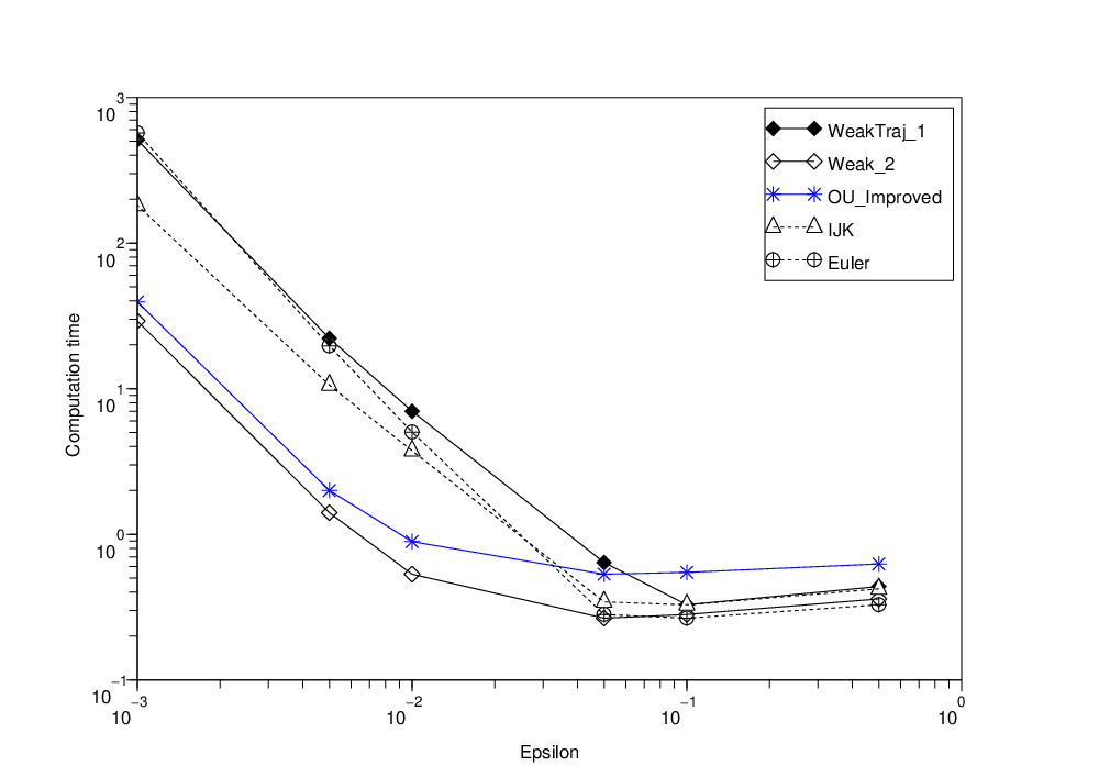
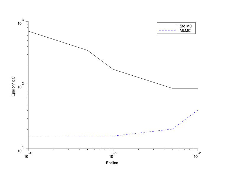
Refer to caption
Figure 13: Multilevel Monte Carlo method for a Call option using different schemes
Refer to caption
Figure 14: OU_Improved scheme with and without multilevel Monte Carlo method

More precisely, for the WeakTraj_1 scheme, consider the interval [k​TN,(k+1)​TN][k\frac{T}{N},(k+1)\frac{T}{N}].
Scheme with time step δ2​N\delta_{2N} :
We approximate mint∈[k​TN,(k+1)​TN]⁡St\min_{t\in[k\frac{T}{N},(k+1)\frac{T}{N}]}S_{t} by m~2​k2​N∧m~2​k+12​N\widetilde{m}^{2N}_{2k}\wedge\widetilde{m}^{2N}_{2k+1} where, ∀0≤j≤2​N−1\forall 0\leq j\leq 2N-1,

m~j2​N=12​(eX~j​T2​N2​N+S(j+1)​T2​Ne,2​N−(eX~j​T2​N2​N−S(j+1)​T2​Ne,2​N)2−2​e2​X~j​T2​N2​N​f2​(Yj​T2​N)​T2​N​ln⁡(Uj)),\widetilde{m}^{2N}_{j}=\frac{1}{2}\left(e^{\widetilde{X}^{2N}_{j\frac{T}{2N}}}+S^{e,2N}_{(j+1)\frac{T}{2N}}-\sqrt{\left(e^{\widetilde{X}^{2N}_{j\frac{T}{2N}}}-S^{e,2N}_{(j+1)\frac{T}{2N}}\right)^{2}-2e^{2\widetilde{X}^{2N}_{j\frac{T}{2N}}}f^{2}(Y_{j\frac{T}{2N}})\frac{T}{2N}\ln(U_{j})}\right),

where S(j+1)​T2​Ne,2​N=eX~j​T2​N2​N​(1+r​T2​N+f⁡(Yj​T2​N)​(ρ⁡(W(j+1)​T2​N−Wj​T2​N)+1−ρ2​(B(j+1)​T2​N−Bj​T2​N)))S^{e,2N}_{(j+1)\frac{T}{2N}}=e^{\widetilde{X}^{2N}_{j\frac{T}{2N}}}\left(1+r\frac{T}{2N}+f(Y_{j\frac{T}{2N}})\left(\rho(W_{(j+1)\frac{T}{2N}}-W_{j\frac{T}{2N}})+\sqrt{1-\rho^{2}}(B_{(j+1)\frac{T}{2N}}-B_{j\frac{T}{2N}})\right)\right) and (Uj)0≤j≤2​N−1(U_{j})_{0\leq j\leq 2N-1} is an independent sequence of independent random variable uniformly distributed.
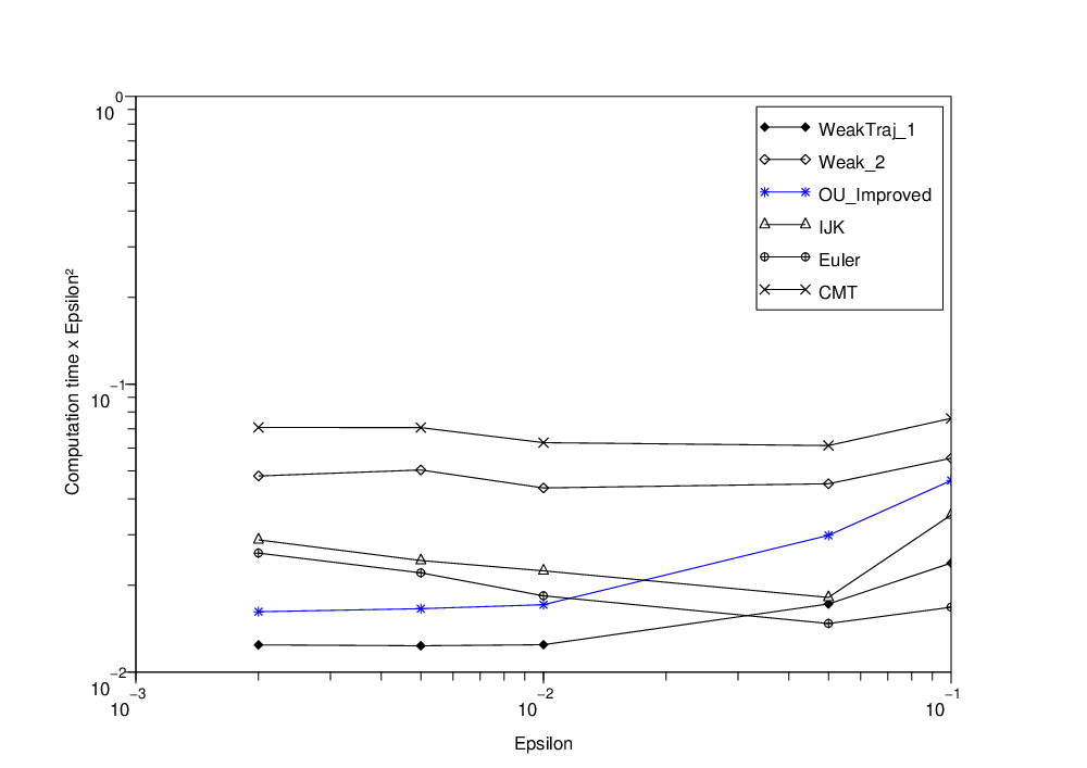
Refer to caption
Figure 15: Multilevel Monte Carlo method for a Lookback option using different schemes.

 
Scheme with time step δN\delta_{N} :
According to Remark 5, X~~tk+1N\widetilde{\widetilde{X}}^{N}_{t_{k+1}} is computed using the Brownian increment Δ​B~k+1N\Delta\widetilde{B}^{N}_{k+1} given by a linear combination of (B(2​k+1)​T2​N−Bk​TN,B(k+1)​TN−B(2​k+1)​T2​N)\left(B_{(2k+1)\frac{T}{2N}}-B_{k\frac{T}{N}},B_{(k+1)\frac{T}{N}}-B_{(2k+1)\frac{T}{2N}}\right) (see (10)). Now, to prevent bias, we are going to approximate mint∈[k​TN,(k+1)​TN]⁡St\min_{t\in[k\frac{T}{N},(k+1)\frac{T}{N}]}S_{t} by the minimum min[tk,tk+1]⁡S~te,2​N\min_{[t_{k},t_{k+1}]}\widetilde{S}^{e,2N}_{t} of some Euler scheme S~te,2​N\widetilde{S}^{e,2N}_{t} like in the scheme with time step δ2​N\delta_{2N}. To remain consistent, we have to choose

S~tk+1e,2​N=eX~~tkN​(1+r​TN+f⁡(Yk​TN)​(ρ⁡(Wtk+1−Wtk)+1−ρ2​Δ​B~k+1N)).\widetilde{S}^{e,2N}_{t_{k+1}}=e^{\widetilde{\widetilde{X}}^{N}_{t_{k}}}\left(1+r\frac{T}{N}+f(Y_{k\frac{T}{N}})\left(\rho(W_{t_{k+1}}-W_{t_{k}})+\sqrt{1-\rho^{2}}\Delta\widetilde{B}^{N}_{k+1}\right)\right).

In order to ensure a good strong coupling with the scheme with time step δ2​N\delta_{2N}, we need to compute the intermediate value S~(2​k+1)​T2​Ne,2​N=eX~~tkN​(1+r​TN+f⁡(Yk​TN)​(ρ⁡(Wtk+1−Wtk)+1−ρ2​Δ​B~~2​k+12​N))\widetilde{S}^{e,2N}_{(2k+1)\frac{T}{2N}}=e^{\widetilde{\widetilde{X}}^{N}_{t_{k}}}\left(1+r\frac{T}{N}+f(Y_{k\frac{T}{N}})\left(\rho(W_{t_{k+1}}-W_{t_{k}})+\sqrt{1-\rho^{2}}\Delta\widetilde{\widetilde{B}}^{2N}_{2k+1}\right)\right) using some Brownian increment Δ​B~~2​k+12​N\Delta\widetilde{\widetilde{B}}^{2N}_{2k+1} as close as possible to B(2​k+1)​T2​N−Bk​TNB_{(2k+1)\frac{T}{2N}}-B_{k\frac{T}{N}} but such that Δ​B~k+1N−Δ​B~~2​k+12​N\Delta\widetilde{B}^{N}_{k+1}-\Delta\widetilde{\widetilde{B}}^{2N}_{2k+1} is independent of Δ​B~~2​k+12​N\Delta\widetilde{\widetilde{B}}^{2N}_{2k+1} and distributed according to 𝒩⁡(0,T2​N)\mathcal{N}(0,\frac{T}{2N}). Choosing Δ​B~~2​k+12​N\Delta\widetilde{\widetilde{B}}^{2N}_{2k+1} of the form a⁡(B(2​k+1)​T2​N−Bk​TN)+b⁡(B(k+1)​TN−B(2​k+1)​T2​N)a2+b2\frac{a\left(B_{(2k+1)\frac{T}{2N}}-B_{k\frac{T}{N}}\right)+b\left(B_{(k+1)\frac{T}{N}}-B_{(2k+1)\frac{T}{2N}}\right)}{\sqrt{a^{2}+b^{2}}} and maximizing C​o​v​(Δ​B~~2​k+12​N,B(2​k+1)​T2​N−Bk​TN)=aa2+b2Cov\left(\Delta\widetilde{\widetilde{B}}^{2N}_{2k+1},B_{(2k+1)\frac{T}{2N}}-B_{k\frac{T}{N}}\right)=\frac{a}{\sqrt{a^{2}+b^{2}}} leads to a=v2​k2​N+v2​k+12​Na=v^{2N}_{2k}+v^{2N}_{2k+1} and b=v2​k+12​N−v2​k2​Nb=v^{2N}_{2k+1}-v^{2N}_{2k} (see Remark 5 for the definition of v2​N.v^{2N}_{.}).

Finally, we approximate mint∈[k​TN,(k+1)​TN]⁡St\min_{t\in[k\frac{T}{N},(k+1)\frac{T}{N}]}S_{t} by m~kN∧m~k+1N\widetilde{m}^{N}_{k}\wedge\widetilde{m}^{N}_{k+1} where

m~kN=12​(eX~~k​TNN+S~(2​k+1)​T2​Ne,2​N−(eX~~k​TNN−S~(2​k+1)​T2​Ne,2​N)2−2​e2​X~~k​TNN​f2​(Yk​TN)​T2​N​ln⁡(U2​k))\widetilde{m}^{N}_{k}=\frac{1}{2}\left(e^{\widetilde{\widetilde{X}}^{N}_{k\frac{T}{N}}}+\widetilde{S}^{e,2N}_{(2k+1)\frac{T}{2N}}-\sqrt{\left(e^{\widetilde{\widetilde{X}}^{N}_{k\frac{T}{N}}}-\widetilde{S}^{e,2N}_{(2k+1)\frac{T}{2N}}\right)^{2}-2e^{2\widetilde{\widetilde{X}}^{N}_{k\frac{T}{N}}}f^{2}(Y_{k\frac{T}{N}})\frac{T}{2N}\ln(U_{2k})}\right)

and

m~k+1N=12​(S~(2​k+1)​T2​Ne,2​N+S~(k+1)​TNe,2​N−(S~(2​k+1)​T2​Ne,2​N−S~(k+1)​TNe,2​N)2−2​e2​X~~k​TNN​f2​(Yk​TN)​T2​N​ln⁡(U2​k+1)).\widetilde{m}^{N}_{k+1}=\frac{1}{2}\left(\widetilde{S}^{e,2N}_{(2k+1)\frac{T}{2N}}+\widetilde{S}^{e,2N}_{(k+1)\frac{T}{N}}-\sqrt{\left(\widetilde{S}^{e,2N}_{(2k+1)\frac{T}{2N}}-\widetilde{S}^{e,2N}_{(k+1)\frac{T}{N}}\right)^{2}-2e^{2\widetilde{\widetilde{X}}^{N}_{k\frac{T}{N}}}f^{2}(Y_{k\frac{T}{N}})\frac{T}{2N}\ln(U_{2k+1})}\right).

The numerical results we obtain are very satisfactory. In figure 15, we draw the CPU time multiplied by the mean square error against the root mean square error. We see that our schemes perform much better than the others.

4 Conclusion

In this article, we have capitalized on the particular structure of stochastic volatility models to propose and discuss two simple and yet competitive discretization schemes. The first one exhibits first order weak trajectorial convergence and has the advantage of improving multilevel Monte Carlo methods for the pricing of path dependent options. The second one is rather useful for pricing European options since it has a second order weak convergence rate.

We have also focused on the special case of an Ornstein-Uhlenbeck process driving the volatility, which encompasses many stochastic volatility models such as the Scott’s model [27] or the quadratic Gaussian model. Then, the convergence properties of the previous schemes are preserved when simulating (Yt)0≤t≤T(Y_{t})_{0\leq t\leq T} exactly. We have also proposed an improved scheme exhibiting both weak trajectorial convergence of order one and weak convergence of order two.

Our numerical experiments confirm the theoretical rates of convergence of our schemes. We also compare the time needed by the different schemes to achieve a given precision in the multilevel Monte Carlo computation of a plain vanilla Call option and a lookback option. For high levels of precision our schemes turn out to be more efficient than the Euler, the Kahl-Jäckel and the Cruzeiro-Malliavin-Thalmaier schemes for both the vanilla Call and the lookback option. The reason is that their better convergence properties compensate the increase of computation effort at each step.

As a last remark, we point out that our results can be naturally extended to stochastic volatility models where the constant correlation coefficient is replaced by a function ρ⁡(Yt)\rho(Y_{t}) of the process driving the stochastic volatility in (1). In this case, if one considers the transformation F(y)=∫.yρ⁡(z)​f​(z)σ⁡(z)dzF(y)=\int_{.}^{y}\frac{\rho(z)f(z)}{\sigma(z)}dz and carries out the same analysis then one should obtain weak trajectorial convergence results under additional regularity assumptions on the function ρ\rho.

References

  • [1] A. Alfonsi. On the discretization schemes for the CIR (and Bessel squared) processes. Monte Carlo Methods and Applications, 11(4):355–384, 2005.
  • [2] A. Alfonsi. High order discretization schemes for the CIR process: Application to affine term structure and Heston models. Mathematics of Computations, 79:209–237, 2009.
  • [3] L. Andersen. Efficient simulation of the heston stochastic volatility model. SSRN eLibrary, 2007.
  • [4] V. Bally and D. Talay. The law of the Euler scheme for stochastic differential equations. I. Convergence rate of the distribution function. Probability Theory and Related Fields, 104(1):43–60, 1996.
  • [5] A. Berkaoui, M. Bossy, and A. Diop. Euler scheme for SDEs with non-Lipschitz diffusion coefficient: strong convergence. ESAIM. Probability and Statistics, 12:1–11, 2008.
  • [6] M. Broadie and Ö Kaya. Exact simulation of stochastic volatility and other affine jump diffusion processes. Operations Research, 54(2):217–231, 2006.
  • [7] A.B. Cruzeiro, P. Malliavin, and A. Thalmaier. Geometrization of Monte-Carlo numerical analysis of an elliptic operator: strong approximation. Comptes Rendus de l’Académie des Sciences. Série I. Mathématique, 338(6):481–486, 2004.
  • [8] G. Deelstra and F. Delbaen. Convergence of discretized stochastic (interest rate) processes with stochastic drift term. Applied Stochastic Models and Data Analysis, 14(1):77–84, 1998.
  • [9] M. Giles. Multilevel Monte Carlo path simulation. Operations Research, 56(3):607–617, 2008.
  • [10] M. Giles. Improved multilevel Monte Carlo convergence using the Milstein scheme. In Monte Carlo and quasi-Monte Carlo methods 2006, pages 343–358. Springer, Berlin, 2008.
  • [11] M. Giles, D. Higham and X. Mao. Analysing multi-level Monte Carlo for options with non-globally Lipschitz payoff. Finance and Stochastics, 13(3):403–413, 2009.
  • [12] J. Guyon. Euler scheme and tempered distributions. Stochastic Processes and their Applications, 116(6):877–904, 2006.
  • [13] J. Hull and A. White. The pricing of options on assets with stochastic volatilities. The Journal of Finance, 42(2):281–300, 1987.
  • [14] C. Kahl and P. Jäckel. Fast strong approximation Monte Carlo schemes for stochastic volatility models. Quantitative Finance, 6(6):513–536, 2006.
  • [15] C. Kahl and H. Schurz. Balanced Milstein methods for ordinary SDEs. Monte Carlo Methods and Applications, 12(2):143–170, 2006.
  • [16] I. Karatzas and S.E. Shreve. Brownian motion and stochastic calculus. Springer-Verlag New-York, 2nd edition, 1991.
  • [17] A. Kebaier. Statistical Romberg extrapolation: a new variance reduction method and applications to option pricing. The Annals of Applied Probability, 15(4):2681–2705, 2005.
  • [18] S. Kusuoka. Approximation of expectation of diffusion process and mathematical finance. Taniguchi Conference on Mathematics Nara ’98, 31:147–165, 2001.
  • [19] S. Kusuoka. Approximation of expectation of diffusion processes based on Lie algebra and Malliavin calculus. Advances in mathematical economics, 6:69–83, 2004.
  • [20] B. Lapeyre and E. Temam. Competitive Monte Carlo methods for pricing Asian options. Journal of Computational Finance, 5(1), 2001.
  • [21] R. Lord, R. Koekkoek, and D.J. Van Dijk. A comparison of biased simulation schemes for stochastic volatility models. SSRN eLibrary, 2008.
  • [22] T. Lyons and N. Victoir. Cubature on Wiener space. Proceedings of The Royal Society of London. Series A. Mathematical, Physical and Engineering Sciences, 460(2041):169–198, 2004.
  • [23] G.N. Milstein. Numerical Integration of Stochastic Differential Equations, volume 313. Kluwer Academic Publishers, 1995.
  • [24] S. Ninomiya and M. Ninomiya. A new higher-order weak approximation scheme for stochastic differential equations and the Runge-Kutta method. Finance and Stochastics, 13:415–443, 2009.
  • [25] S. Ninomiya and N. Victoir. Weak approximation of stochastic differential equations and application to derivative pricing. Applied Mathematical Finance, 15(1-2):107–121, 2008.
  • [26] M. Romano and N. Touzi. Contingent claims and market completeness in a stochastic volatility model. Mathematical Finance, 7(4):399–412, 1997.
  • [27] L.O. Scott. Option pricing when the variance changes randomly: theory, estimation, and an application. The Journal of Financial and Quantitative Analysis, 22(4):419–438, 1987.
  • [28] E.M. Stein and J.C. Stein. Stock price distributions with stochastic volatility: an analytic approach. Review of Financial Studies, 4(4):727–752, 1991.
  • [29] D. Talay and L. Tubaro. Expansion of the global error for numerical schemes solving stochastic differential equations. Stochastic Analysis and Applications, 8(4):483–509, 1990.
  • [30] H. Tanaka and A. Kohatsu-Higa. An operator approach for Markov chain weak approximations with an application to infinite activity Lévy driven SDEs. The Annals of Applied Probability, 19(3):1026–1062, 2009.
  • [31] J.B. Wiggins. Option values under stochastic volatility: Theory and empirical estimates. Journal of Financial Economics, 19(2):351–372, 1987.

5 Appendix

5.1 Proof of Lemma 3

We first suppose that p=1p=1. According to Theorem 5.2 page 72 of Milstein [23], it suffices to check that there exists a positive constant CC independent of NN such that

|𝔼⁡(YδN−Y¯δNN)|≤C​δN2|𝔼⁡((YδN−Y¯δNN)2)|12≤C​δN32|𝔼⁡((YδN−Y¯δNN)4)|14≤C​δN54.\begin{array}[]{rcl}\displaystyle\left|\mathbb{E}\left(Y_{\delta_{N}}-\overline{Y}^{N}_{\delta_{N}}\right)\right|&\leq&\displaystyle C\delta_{N}^{2}\\[8.53581pt] \displaystyle\left|\mathbb{E}\left(\left(Y_{\delta_{N}}-\overline{Y}^{N}_{\delta_{N}}\right)^{2}\right)\right|^{\frac{1}{2}}&\leq&\displaystyle C\delta_{N}^{\frac{3}{2}}\\[8.53581pt] \displaystyle\left|\mathbb{E}\left(\left(Y_{\delta_{N}}-\overline{Y}^{N}_{\delta_{N}}\right)^{4}\right)\right|^{\frac{1}{4}}&\leq&\displaystyle C\delta_{N}^{\frac{5}{4}}.\end{array} (28)

First note that

YδN−Y¯δNN=∫0δNb⁡(Ys)−b⁡(y0)​𝑑s+∫0δN(∫0s(b​σ′+12​σ2​σ′′)​(Yr)​𝑑r+(σ​σ′​(Yr)−σ​σ′​(y0))​d​Wr)​d​Ws.Y_{\delta_{N}}-\overline{Y}^{N}_{\delta_{N}}=\int_{0}^{\delta_{N}}b(Y_{s})-b(y_{0})ds+\int_{0}^{\delta_{N}}\left(\int_{0}^{s}(b\sigma^{\prime}+\frac{1}{2}\sigma^{2}\sigma^{\prime\prime})(Y_{r})dr+(\sigma\sigma^{\prime}(Y_{r})-\sigma\sigma^{\prime}(y_{0}))dW_{r}\right)dW_{s}.

Thanks to Itô’s formula and to assumption (ℋ\mathcal{H}( H 5)), we have that

|𝔼⁡(YδN−Y¯δNN)|=|∫0δN∫0s𝔼⁡((b​b′+12​b′′​σ2)​(Yr))​dr​ds|≤C​|∫0δN∫0sC⁡(1+𝔼⁡(|Yr|2))​dr​ds|≤C​δN2.\begin{array}[]{rcl}\displaystyle\left|\mathbb{E}\left(Y_{\delta_{N}}-\overline{Y}^{N}_{\delta_{N}}\right)\right|&=&\displaystyle\left|\int_{0}^{\delta_{N}}\int_{0}^{s}\mathbb{E}\left((bb^{\prime}+\frac{1}{2}b^{\prime\prime}\sigma^{2})(Y_{r})\right)drds\right|\\[8.53581pt] &\leq&\displaystyle C\left|\int_{0}^{\delta_{N}}\int_{0}^{s}C(1+\mathbb{E}(|Y_{r}|^{2}))drds\right|\\[11.38109pt] &\leq&C\delta_{N}^{2}.\end{array}

Using assumptions (ℋ\mathcal{H}( H 5)) and (ℋ\mathcal{H}( H 6)), we also have ∀p≥1\forall p\geq 1

𝔼⁡(|YδN−Y¯δNN|2​p)≤22​p−1𝔼[|∫0δNb(Ys)−b(y0)ds|2​p+|∫0δN(∫0s(bσ′+12σσ′′)(Yr)dr+(σσ′(Yr)−σσ′(y0))dWr)dWs|2​p]≤22​p−1[δN2​p−1∫0δN𝔼(|b(Ys)−b(y0)|2​p)ds+CδNp−1∫0δN𝔼(|∫0s(bσ′+12σσ′′)(Yr)dr+(σσ′(Yr)−σσ′(y0))dWr|2​p)ds]≤C[δN2​p−1∫0δNspds+δNp−1∫0δNs2​p−1∫0s𝔼(|(bσ′+12σσ′′)(Yr)|2​p)drds+δNp−1∫0δNsp−1∫0s𝔼(|σσ′(Yr)−σσ′(y0)|2​p)drds]≤C​δN3​p.\begin{array}[]{rcl}\displaystyle\mathbb{E}\left(\left|Y_{\delta_{N}}-\overline{Y}^{N}_{\delta_{N}}\right|^{2p}\right)&\leq&\displaystyle 2^{2p-1}\mathbb{E}\left[\left|\int_{0}^{\delta_{N}}b(Y_{s})-b(y_{0})ds\right|^{2p}\right.\\[8.53581pt] &&\displaystyle\quad\quad\left.+\left|\int_{0}^{\delta_{N}}\left(\int_{0}^{s}(b\sigma^{\prime}+\frac{1}{2}\sigma\sigma^{\prime\prime})(Y_{r})dr+(\sigma\sigma^{\prime}(Y_{r})-\sigma\sigma^{\prime}(y_{0}))dW_{r}\right)dW_{s}\right|^{2p}\right]\\[8.53581pt] &\leq&\displaystyle 2^{2p-1}\left[\delta_{N}^{2p-1}\int_{0}^{\delta_{N}}\mathbb{E}\left(|b(Y_{s})-b(y_{0})|^{2p}\right)ds\right.\\[8.53581pt] &&\displaystyle\left.+C\delta_{N}^{p-1}\int_{0}^{\delta_{N}}\mathbb{E}\left(\left|\int_{0}^{s}(b\sigma^{\prime}+\frac{1}{2}\sigma\sigma^{\prime\prime})(Y_{r})dr+(\sigma\sigma^{\prime}(Y_{r})-\sigma\sigma^{\prime}(y_{0}))dW_{r}\right|^{2p}\right)ds\right]\\[8.53581pt] &\leq&\displaystyle C\left[\delta_{N}^{2p-1}\int_{0}^{\delta_{N}}s^{p}ds+\delta_{N}^{p-1}\int_{0}^{\delta_{N}}s^{2p-1}\int_{0}^{s}\mathbb{E}\left(\left|(b\sigma^{\prime}+\frac{1}{2}\sigma\sigma^{\prime\prime})(Y_{r})\right|^{2p}\right)dr\,ds\right.\\[8.53581pt] &&\displaystyle\quad\quad\left.+\delta_{N}^{p-1}\int_{0}^{\delta_{N}}s^{p-1}\int_{0}^{s}\mathbb{E}\left(\left|\sigma\sigma^{\prime}(Y_{r})-\sigma\sigma^{\prime}(y_{0})\right|^{2p}\right)dr\,ds\right]\\[8.53581pt] &\leq&C\delta_{N}^{3p}.\end{array}

This implies both the second and the third inequality of (28). This estimation is also sufficient to extend the result of Milstein [23] to the L2​pL^{2p} norm and conclude the proof.

5.2 Proof of Lemma 8

One can easily check that (Yt)0≤t≤T(Y_{t})_{0\leq t\leq T} is a Gaussian process which has the same distribution law as the process (y0​e−κ​t+θ⁡(1−e−κ​t)+ν​e−κ​t2​κ​We2​κ​t−1)0≤t≤T(y_{0}e^{-\kappa t}+\theta(1-e^{-\kappa t})+\frac{\nu e^{-\kappa t}}{\sqrt{2\kappa}}W_{e^{2\kappa t}-1})_{0\leq t\leq T}. So,

𝔼⁡(ec1​sup0≤t≤T|Yt|1+c2)=𝔼⁡(ec1​sup0≤t≤T|y0​e−κ​t+θ⁡(1−e−κ​t)+ν​e−κ​t2​κ​We2​κ​t−1|1+c2)≤C​𝔼​(eC​sup0≤t≤T|We2​κ​t−1|1+c2).\begin{array}[]{rcl}\displaystyle\mathbb{E}\left(e^{c_{1}\sup_{0\leq t\leq T}|Y_{t}|^{1+c_{2}}}\right)&=&\displaystyle\mathbb{E}\left(e^{c_{1}\sup_{0\leq t\leq T}|y_{0}e^{-\kappa t}+\theta(1-e^{-\kappa t})+\frac{\nu e^{-\kappa t}}{\sqrt{2\kappa}}W_{e^{2\kappa t}-1}|^{1+c_{2}}}\right)\\[8.53581pt] &\leq&\displaystyle C\mathbb{E}\left(e^{C\sup_{0\leq t\leq T}|W_{e^{2\kappa t}-1}|^{1+c_{2}}}\right).\end{array}

Since sup0≤t≤e2​κ​T−1|Wt|=(sup0≤t≤e2​κ​T−1Wt)∨(−inf0≤t≤e2​κ​T−1Wt)\sup_{0\leq t\leq e^{2\kappa T}-1}|W_{t}|=\left(\sup_{0\leq t\leq e^{2\kappa T}-1}W_{t}\right)\vee\left(-\inf_{0\leq t\leq e^{2\kappa T}-1}W_{t}\right), we deduce from the symmetry property of the Brownian motion that

𝔼⁡(ec1​sup0≤t≤T|Yt|1+c2)≤C​𝔼​(eC​|sup0≤t≤e2​κ​T−1Wt|1+c2+eC​|inf0≤t≤e2​κ​T−1Wt|1+c2)≤2​C​𝔼​(eC​|sup0≤t≤e2​κ​T−1Wt|1+c2).\begin{array}[]{rcl}\displaystyle\mathbb{E}\left(e^{c_{1}\sup_{0\leq t\leq T}|Y_{t}|^{1+c_{2}}}\right)&\leq&\displaystyle C\mathbb{E}\left(e^{C|\sup_{0\leq t\leq e^{2\kappa T}-1}W_{t}|^{1+c_{2}}}+e^{C|\inf_{0\leq t\leq e^{2\kappa T}-1}W_{t}|^{1+c_{2}}}\right)\\[5.69054pt] &\leq&\displaystyle 2C\mathbb{E}\left(e^{C|\sup_{0\leq t\leq e^{2\kappa T}-1}W_{t}|^{1+c_{2}}}\right).\end{array}

The probability density function of sup0≤t≤TWt\sup_{0\leq t\leq T}W_{t} is equal to y↦2π​Te−y22​T𝟙{y>0}y\mapsto\sqrt{\frac{2}{\pi T}}e^{-\frac{y^{2}}{2T}}\mathbb{1}_{\{y>0\}} (see for example problem 8.2 p. 96 of Karatzas and Shreve [16]) which permits to conclude.

Let us now assume that y0≠0y_{0}\neq 0. Then t0=definf{t∈[0,T]:y0​e−κ​t+θ⁡(1−e−κ​t)=0}t_{0}\stackrel{{\scriptstyle\rm def}}{{=}}\inf\{t\in[0,T]:y_{0}e^{-\kappa t}+\theta(1-e^{-\kappa t})=0\} (convention inf∅=T\inf\emptyset=T) is positive. ℙ[|Y0|≤N−α]=0\mathbb{P}[|Y_{0}|\leq N^{-\alpha}]=0 for NN large enough and for t∈(0,T]t\in(0,T],

ℙ[|Yt|≤N−α]≤2​N−ανκπ⁡(1−e−2​κ​t)exp(−κ​(|y0​e−κ​t+θ⁡(1−e−κ​t)|−N−α)2ν2​(1−e−2​κ​t)).\displaystyle\mathbb{P}[|Y_{t}|\leq N^{-\alpha}]\leq\frac{2N^{-\alpha}}{\nu}\sqrt{\frac{\kappa}{\pi(1-e^{-2\kappa t})}}\exp\left(-\frac{\kappa(|y_{0}e^{-\kappa t}+\theta(1-e^{-\kappa t})|-N^{-\alpha})^{2}}{\nu^{2}(1-e^{-2\kappa t})}\right).

Since limN→∞inft∈[0,t02](|y0​e−κ​t+θ⁡(1−e−κ​t)|−N−α)>0\lim_{N\to\infty}\inf_{t\in[0,\frac{t_{0}}{2}]}(|y_{0}e^{-\kappa t}+\theta(1-e^{-\kappa t})|-N^{-\alpha})>0, one deduces that supt∈[0,t02]ℙ[|Yt|≤N−α]≤CN−α\sup_{t\in[0,\frac{t_{0}}{2}]}\mathbb{P}[|Y_{t}|\leq N^{-\alpha}]\leq CN^{-\alpha}. The same conclusion holds for supt∈[t02,T]ℙ[|Yt|≤N−α]\sup_{t\in[\frac{t_{0}}{2},T]}\mathbb{P}[|Y_{t}|\leq N^{-\alpha}] by bounding the exponential factor by 11.