CMBR Weak Lensing and HI 21-cm Cross-correlation Angular Power Spectrum
Abstract
Weak gravitational lensing of the CMBR manifests as a secondary anisotropy in the temperature maps. The effect, quantified through the shear and convergence fields imprint the underlying large scale structure (LSS), geometry and evolution history of the Universe. It is hence perceived to be an important observational probe of cosmology. De-lensing the CMBR temperature maps is also crucial for detecting the gravitational wave generated B-modes. Future observations of redshifted 21-cm radiation from the cosmological neutral hydrogen (HI) distribution hold the potential of probing the LSS over a large redshift range. We have investigated the correlation between post-reionization HI signal and weak lensing convergence field. Assuming that the HI follows the dark matter distribution, the cross-correlation angular power spectrum at a multipole is found to be proportional to the cold dark matter power spectrum evaluated at , where denotes the comoving distance to the redshift where the HI is located. The amplitude of the cross-correlation depends on quantities specific to the HI distribution, growth of perturbations and also the underlying cosmological model. In an ideal situation, we found that a statistically significant detection of the cross-correlation signal is possible. If detected, the cross-correlation signal holds the possibility of a joint estimation of cosmological parameters and also may be used to test various CMBR de-lensing estimators.
Keywords:
gravitational lensing; intergalactic media; power spectrumI Introduction
Weak gravitational lensing [1] of distant background sources by intervening large scale structure, distorts their images over large angular scales. The effect arises due to fluctuations of the gravitational potential, and a consequent deflection of light by gravity. Measurement and quantitative study of these distortions allows us to probe the matter distribution and geometry of the universe. Late time evolution of the universe is dictated by dark energy through a modification of the growing mode of perturbations or through possible clustering properties of dark energy ( ). Weak lensing studies can be used to impose constraints on various cosmological parameters and hence, implicitly probe dark energy models [2] and modified gravity theories [3]. It is relevant for our present purpose to note that weak lensing is directly related to the underlying matter distribution of the universe. Weak lensing of background source galaxies by large scale structure (cosmic shear) has been studied extensively, and the measurements have been used for projected mass reconstruction (for review [4]) .
Gravitational lensing also deflects the photons which are free streaming from the last scattering surface (epoch of recombination ) and manifests as a secondary anisotropy in the Cosmic microwave background radiation (henceforth CMBR) brightness temperature maps [5]. Despite, the intrinsic weakness of the ‘signal to noise ratio’ for the above effect, weak lensing of CMBR can, in principle be used to probe the universe at distances () much larger than any galaxy- redshift surveys. Moreover CMBR lensing studies do not face the problems arising due to intrinsic alignment of source galaxies. Standard techniques to measure secondary anisotropies in CMBR, uses the cross correlation of some relevant observable (related to the CMB fluctuations) with fluctuations of some tracer of the large scale structure [6, 7, 8]. Observables relevant to weak lensing are ‘Convergence’ and the ‘Shear’ fields, which quantify the distortion of an image due to gravitational lensing. Convergence () measures the lensing effect through its direct dependence on the gravitational potential and it probes geometry implicitly through its dependence on various cosmological distances.
Future experiments (PLANK 11 1 http://www.rssd.esa.int/index.php?project=planck, CMBPOL [9] etc) would provide high resolution maps for the CMB temperature and polarization fields. The effect of gravitational lensing can be extracted from these maps by constructing various estimators for the convergence field () through quadratic combination of these fields (T, E, B) [10, 11, 12]. One could also predict the noise involved in such estimation based upon various experimental parameters. Lensing reconstruction can also be done using the cm observations [13]. The reconstructed convergence field can then be used for cross correlation. De-lensing the CMB maps is also crucially important for detecting the gravitational wave generated B-mode.
It is well accepted that the the neutral hydrogen (henceforth HI) distribution in the post-reionization epoch () largely traces the underlying large scale structure of the universe [14, 15, 16]. This allows us to relate HI distribution to the cold dark matter distribution through a possible ‘bias’. Matter perturbations are in the linear regime on large scales under consideration and the above simplifying assumption is reasonable. Hence, observations of the redshifted radiation of the HI spin-flip hyperfine transition provides an unique opportunity for probing the universe over a wide range of redshifts () [14, 15, 16]. Theoretical predictions [17, 18] have suggested the use of HI, statistically, as a probe of large scale structure. Positive correlation between the optical galaxies (6dFGS) and HI fluctuations [19] has also been observed recently.
In this paper we have investigated the possibility of using diffused cosmological HI as a tracer of the underlying large scale structure to probe weak lensing induced secondary anisotropy of the CMBR. Cosmic shear fields imprint the underlying distribution of matter over large scales. We have studied the the cross correlation between the post-reionization fluctuations in the HI brightness temperature and the weak lensing convergence field. The cross-correlation angular power spectrum, measures the strength of the correlation as a function of the angular scale.
The weak lensing of CMBR, quantified through the convergence field is expressed as a line of sight integral. Cross correlation of weak lensing with the HI fluctuations, however pick up the contribution from only one redshift ( at which the HI is probed). The advantage of using HI observations is that, the redshifted line emission observations allow us to probe the universe continuously at different redshifts. We can probe the integral effect of weak lensing at any intermediate redshift by suitably tuning the frequency band for HI observation. This, in principle enables us to do a tomographic study of the late-time cosmic history continuously over an entire range of redshifts. On similar lines, cross-correlation of HI temperature map with the CMBR, aimed to isolate the ISW signal (an integral effect) has been studied [20].
Several Radio telescopes (eg.currently functioning GMRT 22 2 http://www.gmrt.ncra.tifr.res.in/ and upcoming MWA 33 3 http://www.haystack.mit.edu/ast/arrays/mwa/ & LOFAR 44 4 http://www.lofar.org/) are aimed to map the cosmological distribution of HI at high redshifts. The extreme weakness of the post-reionization HI signal () from individual clouds, despite some magnification due to Gravitational lensing [21], poses a serious observational challenge. However, observation of the statistical distribution of HI as a weak background in radio observations does not require the need to resolve individual galaxies. Such observations contain information about the HI fluctuations at the comoving distance being probed (frequency) [17, 18].
Convergence field reconstructed from CMBR maps of large portion of the sky and a corresponding HI map would allow us to compute the cross-correlation power spectrum and hence independently quantify the cosmic history at redshifts . The cross-correlation power spectrum may also independently compare the various theoretical estimators that separate the lensing contribution from the CMB data .
II Formulation
The lensed CMB brightness temperature along the direction of the unit vector is related to the unlensed temperature through the map , where denotes the total deflection due to weak lensing by the intervening large scale structure. At the lowest order, magnification of the signal is given by the convergence, .The convergence field can be written as a line of sight integral given by [1]
| (1) |
where stands for the comoving angular diameter distance and is given by
| (2) |
Here denotes the growing mode for the density contrast , and denotes the conformal time corresponding to the last scattering surface (assuming instantaneous recombination), and denotes the scale factor.
Here we have excluded weaker contribution to the convergence field from sources other than large scale structure (like gravitational waves). Expanding this in the basis of spherical harmonics
| (3) |
The expansion coefficients can be obtained by integrating over the solid angle as
| (4) |
Using the Raleigh expansion
| (5) |
we have
| (6) |
where is the Fourier transform of , and is the spherical Bessel function.
In studying the post-reionization HI power spectrum we assume that the HI traces the underlying dark matter distribution with a possible bias function , where and denote the HI and dark matter power spectra respectively. This function is assumed to quantify the clustering property of the neutral gas. It is believed that, on small scales (below the Jean’s length), the linear density contrast for the gas is related to the dark matter density contrast though a scale dependent function [22]. However the bias is known to be reasonably scale-independent on large scales. The length scale above which the bias is linear, depends crucially on the redshift being probed. Numerical simulations indicate that the large scale linear bias grows monotonically with redshift for [23]. This is known to be true for galaxies [24, 25, 26]. The increase in the amplitude of HI brightness temperature power spectrum is however slow (a factor of for z between and )[27]. In this paper we have considered scales which are much larger than the scale of non-linearity and hence linear scale independent bias has been used.
Expanding the HI 21-cm brightness temperature fluctuations (in Fourier space [28]) from redshift in terms of spherical harmonics and proceeding as before we get
| (7) |
where is the mean HI fraction, and
| (8) |
The term has its origin in the HI peculiar velocities [17, 28] which have also been assumed to be caused by the dark matter fluctuations. In equation (7) we have defined
| (9) |
Where denotes the logarithmic derivative of the growing mode and is given by .
At redshifts we have (for details see [29, 30, 31]). This allows us to calculate the mean neutral fraction of the hydrogen gas , which we assume is a constant over the entire redshift range .
We use equations (6) and (7) to calculate , the cross correlation angular power spectrum between the HI 21-cm brightness temperature signal and the convergence field, defined through
| (10) |
Note that also depends on , the redshift from which the HI signal originates, or equivalently on , the frequency of the HI observations (not explicitly mentioned here).
We obtain
| (11) |
where is the present day dark matter power spectrum,
| (12) |
For large (small angular scales where “flat sky” approximation is reasonable) the Limber approximation in Fourier space [32, 33], , allows us to understand various generic scaling properties of the angular cross-correlation power spectrum.
| (13) |
where is the present day dark matter power spectrum and all the terms on the rhs. are evaluated at .
Using equation (6) we have the Convergence auto-correlation power spectrum which for large can be approximately written as
| (14) |
We also have, for comparison, the HI-HI angular power spectrum [35], which describes the statistical properties of HI fluctuations .
The function is known to be a direct observational estimator of the HI fluctuations at redshift and does not require the assumption of an underlying cosmological model (eg. [34]). Using the ‘flat sky’ approximation [35], which is reasonable for , we have given by
| (15) |
where is the comoving distance corresponding to the redshift or equivalently frequency , and . In this paper we have used the WMAP data for the various cosmological parameters.
We note that the quantity of interest - the convergence field , is not a direct observable in CMBR experiments. The degree of non-gaussianity in the lensed CMB maps is proportional to the lensing potential responsible for it. This allows a reconstruction of the weak lensing potential and consequently the deflection angle , through the use of various statistical estimators [36, 37]. The reconstructed lensing convergence field is sensitive to the statistical tool (estimator) being used and reflects the degree of de-lensing achieved.
The estimated quantity, we have focussed on, namely the cross correlation angular power spectrum, , does not directly de-lens the CMB maps. It however uses the reconstructed convergence field, and is hence sensitive to the underlying de-lensing technique, and the cosmological model. We have calculated the theoretical cross-correlation power spectrum assuming a standard cosmological model. The estimated , (where is the estimated convergence field) with its known error bars can be compared with our predicted . Hence, the theoretical cross-correlation angular power spectrum provides a template to independently compare various estimators which are aimed at de-lensing the CMB maps.
III Results
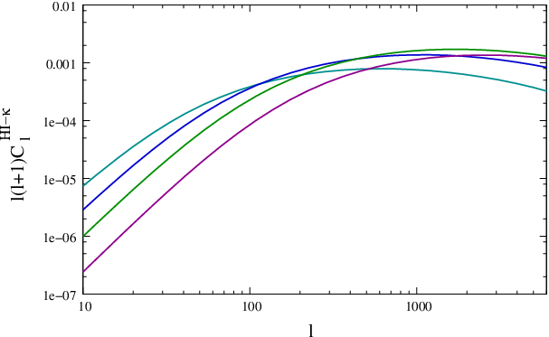

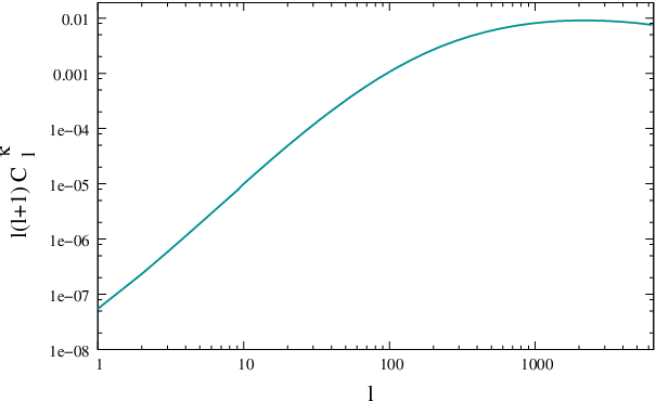
Figure 1 shows the theoretically predicted cross-correlation angular power spectrum for various redshifts . The currently favored CDM cosmological model with parameters (, , , , ) [38, 39] has been used here. For HI signal we have assumed a linear bias model (reasonable on the large scales under consideration) with in the fiducial model.
Numerical simulations have indicated the deviation from at high redshifts. It is seen that at large scales the linear bias is for . The effect of larger (scale independent) bias is shown in figure 2. Apart from the scaling of the power spectrum at large scales the bias also has a weak effect of modifying the power spectrum amplitude through the change in the the redshift space distortion factor . We have also indicated the scale , above which the linear bias assumtion is invalid. For this angular scale . We have restricted ourselves to multipoles less than that.
Figure 3 shows the Convergence auto-correlation power spectrum for reference. The Cross-correlation power spectrum has the same shape as the matter power spectrum. For different redshifts the signal peaks at a particular which scales as . The angular distribution of power clearly follows the underlying clustering properties of matter. The amplitude of the cross-correlation power spectrum depends on various factors some of which are related to the underlying cosmological model and others related to the HI distribution at . The angular diameter distances directly imprint the geometry of the universe and also depends on the cosmological parameters. The signal has been proposed to be an useful probe of the cosmological parameters [40, 41, 42]. The cross-correlation signal may likewise be used independently for joint estimation of parameters.
We shall now discuss the prospect of detecting the cross-correlation signal. Redshifted cm signal is buried deep under foregrounds. Removal of the foreground component is a major challenge [34, 35, 42, 43]. However, it is to be noted that cross-correlation between the HI brightness temperature field and the convergence field is much less likely to be affected by foregrounds or other systematics. The error in the cross-correlation signal is a sum in quadrature, of the contribution due to instrumental noise and sample variance. Increased resolution (for CMB experiment) and increased time of observation (for 21 cm observation) can in principle significantly reduce the instrumental noise. Sample variance however puts a fundamental bound on the detectability of the signal.
The sample variance for the cross-correlation angular power spectrum is given by
| (16) |
Where the numerator contains the auto-correlation angular power spectra. represents a band in and is fraction of sky common to the convergence field and HI brightness temperature distribution . denotes the number of independent estimates of the cm observations obtained from different frequency channels in a given frequency band and suppresses the sample variance by a factor .
We have used the ideal hypothetical possibility of , and used . we have chosen assuming that the HI signal decorrelates over a frequency separation of and hence yield independent estimates for a bandwidth radio observation. The estimated Signal to Noise ratio is shown in fig 4 . for . The predicted is seen to be and is not high enough for a statistically significant detection which requires . Choosing a for and for will however produce a .
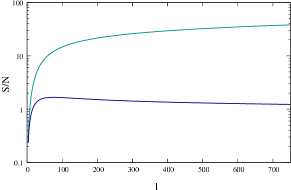
It is possible to increase the by collapsing the signal from different scales and thereby test the feasibility of a statistically significant detection. The Signal to Noise cumulated upto a multipole is defined as (see [44] for similar calculation)
| (17) |
The summation in the above equation extends up to a certain . and denotes the noise power spectrum for and HI observations respectively. Ignoring the instrument noises we note that there is a significant increase in the by cumulating over multipoles . This implies that a statistically significant detection of is possible and the signal is not cosmic variance limited. - cm observations allow us to probe a continuous range of redshifts. This allows us to further increase the by collapsing the signal from various redshifts. As discussed earlier, an increased HI bias would increase the signal. However the is not expected to be seriously affected.
Instrumental noise plays an important role at large multipoles (small scale). For a typical CMB experiment, the noise power spectrum [45, 46] is given by , where different pixels are assumed to have uncorrelated noise with uniform variance , where and denotes pixel sensitivity and ‘time spent on the pixel’ respectively. is the solid angle subtended per pixel and we choose a gaussian beam . For CMBPOL [9] like experiments, the noise power spectrum for with the beam FWHM and sensitivity is for (see [47, 9]) Hence, and maybe ignored in our present analysis.
For HI observations, the quantity of interest is the complex Visibility which is used to estimate the power spectrum [34]. For a radio telescope with N antennae, system temperature , operating at a frequency , and band width the noise correlation is given by [48]
| (18) |
Where , denotes total observation time, and is related to the effective collecting area of the antenna dish . The function takes any non-uniform distribution of baselines into account and depends on the array design. The bin is chosen assuming a gaussian beam of width . With a GMRT or MWA like instrument [34], one can in principle achieve a noise level much lesser than the signal by increasing the time of observation (a 2000 hour observation is sufficient even with the present GMRT cofiguration) and also by increasing the band width of the instrument. Being inversely related to the number of antennae in the array, future designs can allow further suppression of the the system noise and achieve .
This establishes the detectability of the cross-correlation signal. We would like to conclude by noting that this theoretical prediction of positive correlation between weak lensing fields and 21 cm maps, quantified through may allow an independent means to estimate various cosmological parameters and also test various estimators for CMBR delensing.
IV Acknowledgments
T.G.S would like to acknowledge Somnath Bharadwaj for useful discussions and help. Authors also acknowledge financial support from the Board of Research in Nuclear Sciences (BRNS), Department of Atomic Energy (DAE), Government of India.
References
- [1] Van Waerbeke, L., & Mellier, Y., arXiv:astro-ph/0305089 (2003)
- [2] Hoekstra, H., & Jain, B., Annual Review of Nuclear and Particle Science, 58, 99 (2008)
- [3] Schmidt, F., PRD, 78, 043002 (2008)
- [4] Munshi, D., Valageas, P., Van Waerbeke, L., & Heavens, A., arXiv:astro-ph/0612667 (2006)
- [5] Lewis, A., & Challinor, A., Phys.Rept., 429, 1 (2006)
- [6] Hirata, C. M., Padmanabhan, N., Seljak, U., Schlegel, D., & Brinkmann, J., PRD, 70, 103501 (2004)
- [7] Smith, K. M., Zahn, O., & Doré, O., PRD, 76, 043510 (2007)
- [8] Hirata, C. M., Ho, S., Padmanabhan, N., Seljak, U., & Bahcall, N. A., PRD, 78, 043520 (2008)
- [9] Smith, K. M., et al. , arXiv:0811.3916 (2008)
- [10] Hu, W. , ApJL, 557, L79 (2001)
- [11] Seljak, U., & Zaldarriaga, M. Physical Review Letters, 82, 2636 (1999)
- [12] Hu, W., & Okamoto, T., ApJ, 574, 566 (2002)
- [13] Zahn, O., & Zaldarriaga, M. ApJ, 653, 922 (2006)
- [14] Bharadwaj, S., & Ali S. S., MNRAS, 356, 1519 (2005)
- [15] Furlanetto , S. R. , Oh ,S. P.,. & Briggs,F., Phys.Rept. 433, 181 (2006)
- [16] Lewis, A., & Challinor, A., PRD, 76, 083005 (2007)
- [17] S. Bharadwaj, B. B. Nath, & S. K. Sethi, JApA, 22, 21 (2001)
- [18] S. Bharadwaj & S. K. Sethi, JApA, 22, 293 (2001)
- [19] Pen, U.-L., Staveley-Smith, L., Peterson, J., & Chang, T.-C. astro-ph/0802.3239
- [20] Guha Sarkar, T., Datta, K. K., & Bharadwaj, S. 2008, arXiv:0810.3649
- [21] Saini T., Bharadwaj S. & Sethi, K. S. , ApJ, 557, 421 (2001)
- [22] Fang L.Z.,Bi H., Xiang S., Borner G., ApJ 413, 477 (1993)
- [23] Marin, F., Gnedin, N. Y., Seo, H.-J., & Vallinotto, A. 2009, arXiv:0911.0041
- [24] Fry J. N., ApJ, 461, L65 (1996)
- [25] Mo H. J., White S. D. M., MNRAS, 282, 347 (1996)
- [26] Mo H. J., Mao S., White S. D. M., MNRAS, 304, 175 (1999)
- [27] Bagla, J. S., & Khandai, N., arXiv:0908.3796 (2009)
- [28] Bharadwaj, S., & Ali, S. S., , MNRAS, 352, 142 (2004)
- [29] Péroux, C., McMahon, R. G., Storrie-Lombardi, L. J. & Irwin, M .J., MNRAS, 346, 1103 (2003)
- [30] Storrie–Lombardi, L. J., McMahon, R. G., Irwin, M. J., MNRAS, 283, L79 (1996)
- [31] Lanzetta, K. M., Wolfe, A. M., Turnshek, D. A., ApJ, 430, 435 (1995)
- [32] Limber, D.N., ApJ , 119, 655 (1954)
- [33] Afshordi, N., Loh, Y.-S., & Strauss, M. A., PRD, 69, 083524 (2004)
- [34] Ali, S. S., Bharadwaj, S., & Chengalur, J. N., MNRAS, 385, 2166 (2008)
- [35] Datta, K. K., Choudhury, T. R., & Bharadwaj, S., MNRAS, 378, 119 (2007)
- [36] Hanson, D., Challinor, A., & Lewis, A., arXiv:0911.0612 (2009)
- [37] Kesden, M., Cooray, A., & Kamionkowski, M., PRD, 67, 123507 (2003)
- [38] Tegmark, M., et al., PRD, 69, 103501
- [39] Komatsu, E., et al., Astrophys.J.Suppl, 180, 330 (2009)
- [40] Bharadwaj, S., Sethi, S. K., & Deep Saini, T., astro-ph/0809.0363
- [41] Wyithe, S., & Loeb, A., astro-ph/0808.2323
- [42] McQuinn, M., Zahn, O., Zaldarriaga, M., Hernquist, L., & Furlanetto, S. R., ApJ, 653, 815 (2006)
- [43] Santos, M. G., Cooray, A., & Knox, L., ApJ, 625, 575 (2005)
- [44] Cooray, A., PRD, 65, 103510 (2002)
- [45] Marian, L., & Bernstein, G. M., PRD, 76, 123009 (2007)
- [46] Smith, K. M., Hu, W., & Kaplinghat, M., PRD, 74, 123002 (2006)
- [47] Das, S., & Spergel, D. N., PRD, 79, 043509 (2009)
- [48] Khandai, N., Datta, K. K., & Bagla, J. S., arXiv:0908.3857 (2009)