Congestion in a macroscopic model of self-driven particles modeling gregariousness

Our starting point is the following model, written in dimensionless form:

	$\displaystyle\partial_{t}\rho+\nabla_{\vec{x}}\cdot(\rho\Omega)=0,$		(2.1)
	$\displaystyle\partial_{t}\Omega+(\Omega\cdot\nabla_{\vec{x}})\Omega+(\mbox{Id}-\Omega\otimes\Omega)\nabla p(\rho)=0.$		(2.2)

where $\rho=\rho(\vec{x},t)$ is the particle density and $\Omega=\Omega(\vec{x},t)$ is the particle velocity. The problem is posed on the 2-dimensional plane $\vec{x}\in\mathbb{R}^{2}$ and $t>0$ is the time. The velocity $\Omega(\vec{x},t)\in\mathbb{R}^{2}$ is supposed to satisfy the normalization constraint

$$|\Omega(\vec{x},t)|=1,\ \forall\vec{x}\in\mathbb{R}^{2},\ \forall t>0.$$

(2.3)

Therefore, $\Omega(\vec{x},t)\in\mathbb{S}^{1}$, the unit sphere, at any point in space-time. The function $p(\rho)$ is an increasing function such that $p(\rho)\sim\rho^{\gamma}$ when $\gamma\ll 1$ and $p(\rho)\rightarrow+\infty$ when $\rho\rightarrow\rho^{\ast}$ where $\rho^{\ast}$ is the so-called congestion density. In this paper, we will consider

$$p(\rho)=\frac{1}{\left(\frac{1}{\rho}-\frac{1}{\rho^{\ast}}\right)^{\gamma}},$$

(2.4)

for simplicity but any other function with similar behaviour would lead to similar results. The operators $\nabla_{\vec{x}}\cdot$ and $(\Omega\cdot\nabla_{\vec{x}})$ are defined, for a vector field $\vec{A}=(A_{1},A_{2})(\vec{x})$, by

	$\displaystyle\nabla_{\vec{x}}\cdot\vec{A}=\partial_{x_{1}}A_{1}+\partial_{x_{2}}A_{2},$		(2.5)
	$\displaystyle(\Omega\cdot\nabla_{\vec{x}})\vec{A}=((\Omega_{1}\partial_{x_{1}}+\Omega_{2}\partial_{x_{1}})A_{1},(\Omega_{1}\partial_{x_{1}}+\Omega_{2}\partial_{x_{1}})A_{2})^{T},$		(2.6)

where $T$ denotes the transpose operator. Finally, $(\mbox{Id}-\Omega\otimes\Omega)$ is the projection matrix onto the line spanned by $\Omega^{\perp}$, where $\Omega^{\perp}$ is the vector $\Omega$ rotated by the angle $\pi/2$. Alternatively, we have, for a vector $\vec{A}$:

$$(\mbox{Id}-\Omega\otimes\Omega)\vec{A}=\vec{A}-(\Omega\cdot\vec{A})\vec{A},$$

(2.7)

where $(\Omega\cdot\vec{A})$ is the dot product $\Omega\cdot\vec{A}=\Omega_{1}A_{1}+\Omega_{2}A_{2}$.

We show in appendix $A$ that this model well describes the behaviour of a system of particles subjected to long-range attraction and short-range repulsion in the spirit of a model proposed by Aoki [1] or Couzin et al [16] for modelling gregariousness and swarming. More precisely, in appendix $A$, we derive this system from such a particle system through successive changes of scales via mean-field and hydrodynamic theories. In the form (2.2), we have dropped the force term describing long-range attraction. Indeed, this force term would add the quantity $(\mbox{Id}-\Omega\otimes\Omega)\vec{\vec{\xi}}_{a}$ at the right-hand side of (2.2), with

$$\vec{\xi_{a}}(\vec{x},t)=\frac{\int K_{a}(|\vec{y}-\vec{x}|)(\vec{y}-\vec{x})\rho(\vec{y},t)d\vec{y}}{\int K_{a}(|\vec{y}-\vec{x}|)\rho(\vec{y},t)d\vec{y}},$$

where $K_{a}$ is a bounded positive kernel. This terms does not add any differential operator and all the subsequent analysis will stay unaltered by adding this term.

Our main concern is the study of the congestion effects brought by the singularity of $p(\rho)$ near the congestion density $\rho^{\ast}$. Indeed, a herd of animals can be viewed, at large scales, as a domain of space where the density $\rho$ is close to the saturation density $\rho^{\ast}$. Therefore, the geometrical domain occupied by the herd at time $t$ can be identified to a set $H_{t}=\{x\in{\mathbb{R}}^{2}\,|\,\rho^{*}-\delta\rho<\rho(x,t)<\rho^{*}\}$ where the parameter $\delta\rho>0$ must be suitably tuned. Therefore, with the initial model (2.1), (2.2), the definition of a herd depends on an arbitrary parameter $\delta\rho$, which makes it ambiguous.

A way to unambiguously define the herd is to force the system (2.1)-(2.2) to make clear-cut phase transitions from unclustered $\rho<\rho^{\ast}$ to clustered $\rho=\rho^{\ast}$ phases. In the spirit of the works [6, 20, 7] for traffic, this can be achieved in an asymptotic regime which amounts to supposing that there is merely no repulsive interactions at all as long as $\rho<\rho^{\ast}$, and that repulsive ”pressure” forces turn on suddenly when $\rho$ hits the congestion density $\rho^{\ast}$. This can be done by rescaling $p(\rho)$ into $\varepsilon p(\rho)$ where $\varepsilon\ll 1$ is a small parameter. In this way, repulsive interactions are $O(\varepsilon)$ as long as $\rho<\rho^{\ast}$, but become $O(1)$ when $\rho=\rho^{\ast}$ (see fig. 1).

Biologically, this assumption amounts to saying that the animals do not change their directed motion by the presence of their neighbours unless they touch them and need to modify their trajectory to bypass them. The parameter $\varepsilon\ll 1$ is related to the time scale at which this change of trajectory occurs and is therefore supposed small. Let us also note that our model considers that all animals move with speed unity and never stop. Obviously the model will require improvements by taking into account the fact that a certain fraction of animals are steady, while foraging or resting.

Therefore, our main concern in this paper is the study of the following perturbation problem:

	$\displaystyle\partial_{t}\rho^{\varepsilon}+\nabla_{\vec{x}}\cdot(\rho^{\varepsilon}\Omega^{\varepsilon})=0,$		(2.8)
	$\displaystyle\partial_{t}\Omega^{\varepsilon}+(\Omega^{\varepsilon}\cdot\nabla_{\vec{x}})\Omega^{\varepsilon}+\varepsilon(\mbox{Id}-\Omega^{\varepsilon}\otimes\Omega^{\varepsilon})\nabla_{\vec{x}}p(\rho^{\varepsilon})=0,$		(2.9)
	$\displaystyle|\Omega^{\varepsilon}|=1.$		(2.10)

We will be interested in the formal limit $\varepsilon\rightarrow 0$. A rigorous theory of this type of problems is unfortunately still out of reach up to our knowledge. In the following section, we show that the limit $\varepsilon\rightarrow 0$ leads to a phase transition between compressible and incompressible regimes.

As $\varepsilon\rightarrow 0$, $\varepsilon p(\rho^{\varepsilon})$ becomes significant only where the convergence $\rho^{\varepsilon}\rightarrow\rho^{\ast}$ is fast enough. Therefore, in the limit, either $\rho^{\varepsilon}\rightarrow\rho<\rho^{\ast}$ and $\varepsilon p(\rho^{\varepsilon})\rightarrow 0$ or $\rho^{\varepsilon}\rightarrow\rho^{\ast}$ and $\varepsilon p(\rho^{\varepsilon})\rightarrow\bar{p}$ with $\bar{p}$ possibly non zero. In other words, the equation $(\rho^{\ast}-\rho)\bar{p}=0$ holds in the limit. If additionally $\bar{p}<+\infty$, straighforward inspection shows that

$$\rho^{\ast}-\rho^{\varepsilon}=O(\varepsilon^{\frac{1}{\gamma}}).$$

(2.11)

Therefore, the formal limit $\varepsilon\rightarrow 0$ of system (2.8)-(2.9)-(2.10) is given by the following system:

	$\displaystyle\partial_{t}\rho+\nabla_{\vec{x}}\cdot(\rho\Omega)=0,$		(2.12)
	$\displaystyle\partial_{t}\Omega+\Omega\cdot\nabla_{\vec{x}}\Omega+(\mbox{Id}-\Omega\otimes\Omega)\nabla_{\vec{x}}\bar{p}=0,$		(2.13)
	$\displaystyle|\Omega|=1,$		(2.14)
	$\displaystyle(\rho^{\ast}-\rho)\bar{p}=0.$		(2.15)

In the non-congested domain $\rho<\rho^{\ast}$, the system reduces to a pressureless compressible gaz dynamics model with a speed constraint

	$\displaystyle\partial_{t}\rho+\nabla_{\vec{x}}\cdot\rho\Omega=0,$		(2.16)
	$\displaystyle\partial_{t}\Omega+\Omega\cdot\nabla_{\vec{x}}\Omega=0,$		(2.17)
	$\displaystyle|\Omega|=1.$		(2.18)

This system describes the behaviour of the system outside the congested region. It is a compressible system. Biologically, it describes the behaviour of dispersed animals outside the herd. Mathematical studies of this system are outside the scope of this article and the reader can refer to [9] for standard pressureless gas dynamics models (without speed constraint). We note that this system exhibits vacuum regions where $\rho=0$ as it will be seen below.

The congested part of the flow is defined as the region where the congestion constraint $\rho=\rho^{\ast}$ is reached. Biologically, it defines the domain of space occupied by the herd. Its connected components will be called ”clusters”. In the congested domain, system (2.12)-(2.15) turns into an incompressible Euler model with speed constraint:

	$\displaystyle\nabla_{\vec{x}}\cdot\Omega=0,$		(2.19)
	$\displaystyle\partial_{t}\Omega+\Omega\cdot\nabla_{\vec{x}}\Omega+(\mbox{Id}-\Omega\otimes\Omega)\nabla_{\vec{x}}\bar{p}=0.$		(2.20)
	$\displaystyle|\Omega|=1,$		(2.21)
	$\displaystyle\rho=\rho^{\ast},$		(2.22)

We first note that smooth incompressible vector fields of constant norm in $\mathbb{R}^{2}$ have a very special structure which is outlined in the following.

The proof of this proposition simply results from introducing the angle $\theta$ so that $\Omega(\vec{x},t)=(\cos(\theta(\vec{x},t)),\sin(\theta(\vec{x},t)))$ and noting that $\theta$ satisfies the ”transport equation”

$$\partial_{x_{2}}\theta-(\tan\theta)\partial_{x_{1}}\theta=0.$$

This property implies that the knowledge of $\Omega$ on the cluster boundaries suffices to know $\Omega$ everywhere inside the clusters.

The integral curves of $\Omega$ provide a mathematical description of the animal files in the herd. These curves being parallel to each other, they are consistant with the intuition and the observation of animal files in a herd (see fig. 2).

The pressure $\bar{p}$ satisfies an elliptic equation. Indeed, by taking the divergence of the equation (2.20) and after easy computations, we get

$$\nabla_{\vec{x}}\cdot\left(\left(\mbox{Id}-\Omega\otimes\Omega\right)\nabla_{\vec{x}}\bar{p}\right)=\text{Tr}((\nabla_{\vec{x}}\Omega)(\nabla_{\vec{x}}\Omega)^{T}),$$

(2.23)

where Tr is the trace of a matrix and the exponent $T$ denotes the transpose operator. This equation can be equivalently written:

$$-(\Omega^{\perp}\cdot\nabla_{\vec{x}})^{2}\bar{p}-(\nabla_{\vec{x}}\cdot\Omega^{\perp})(\Omega^{\perp}\cdot\nabla_{\vec{x}})\bar{p}=-\text{Tr}((\nabla_{\vec{x}}\Omega)(\nabla_{\vec{x}}\Omega)^{T}),$$

(2.24)

and only involves the operator $(\Omega^{\perp}\cdot\nabla_{\vec{x}})$ applied to $\bar{p}$. Since the integral lines of $\Omega^{\perp}$ are straight lines, equation (2.24) is just a one-dimensional elliptic problem for $\bar{p}$ posed on this straight line. Knowing the boundary values of $\bar{p}$ where this straight line meets the boundary of the cluster allows to compute $\bar{p}$ everywhere on this lines and consequently inside the cluster (see fig. 2). Hence, once $\Omega$ is known inside the cluster, the resolution of this equation only requires the knowledge of the boundary conditions for $\bar{p}$ at the boundaries of the cluster.

To close the system, i.e. to determine how the solution in the congested domain evolves, we need to determine these boundary conditions. They are not given by the formal limit and, in order to determine them, we need to explore another route. For this pupose we look at the solutions of the Riemann problem for the perturbed and limit systems. Note that if we abandon the constraint of constant norm $|\Omega|=1$, the non conservative term $(\Omega\otimes\Omega)\nabla_{\vec{x}}\bar{p}$ in the momentum conservation equation (2.13) drops out, and we recover a conservative model expressing mass and momentum equation. Then, the Rankine-Hugoniot conditions across the boundary between the compressible and incompressible regions provide the boundary conditions for the pressure at the cluster boundary. The constant norm constraint prevents from using this strategy. Therefore, we need to find a different route to specify these boundary conditions.

To find the boundary conditions on the cluster boundaries, we need to extract more information from the perturbation system (2.8)-(2.10) than the mere limit system (2.12)-(2.15). As such, this system is underdetermined. The strategy is to extract such information by passing to the limit $\varepsilon\rightarrow 0$ in some special solutions of this system. To underline the difficulty resulting from the non-conservativity, let us first look at the Rankine-Hugoniot conditions. We have the following proposition.

The proof of this proposition is omitted. The second relation provides us information when the mean velocity is not tangent to the cluster. In this condition, if the mean velocity is continuous, the pressure is also continuous. This implies that the pressure is zero on a cluster boundary if the mean velocity is continuous. This fact will be supported by the forthcoming analysis. However, as regards the interface dynamics, such an analysis is incomplete because the second equation supposes that $\Omega$ is continuous.

So as to capture the correct boundary conditions for the pressure $\bar{p}$ and the velocity $\Omega$ at a cluster boundary where $\rho$ and $\Omega$ may be discontinuous, we consider a one dimensional problem in the normal direction $n$ to this boundary (cf. figure 3). In order to justify this simplication, we introduce the coordinate system $(x_{1},x_{2})$ in the normal and tangent direction to the boundary. The angle $\theta$ is defined so that $\Omega(\vec{x},t)=(\cos(\theta(\vec{x},t)),\sin(\theta(\vec{x},t)))$ in this basis. System (2.8)-(2.9) then becomes (the index $\varepsilon$ is omitted):

	$\displaystyle\hskip-34.14322pt\partial_{t}\rho+\partial_{x_{1}}(\rho\cos\theta)+\partial_{x_{2}}(\rho\sin\theta)=0,$		(2.27)
	$\displaystyle\hskip-34.14322pt\left[\partial_{t}\theta+(\cos\theta\partial_{x_{1}}\theta+\sin\theta\partial_{x_{2}}\theta)+\left(-\sin\theta\partial_{x_{1}}\varepsilon p(\rho)+\cos\theta\partial_{x_{2}}\varepsilon p(\rho)\right)\right]\left(\begin{array}[]{c}-\sin\theta\\ \cos\theta\end{array}\right)=0.$

We suppose that all quantities have locally smooth variations in the direction tangent to the boundary and we focus on the possible sharp variations or discontinuities in the normal direction. To analyze this situation, we perform a coordinate dilation in the $x_{1}$ direction and in time: $x_{1}^{\prime}=\delta x_{1}$, $x_{2}^{\prime}=\delta x_{2}$, $t^{\prime}=\delta t$, with $\delta\ll 1$. In these new variables, all $x_{1}$ and $t$ derivatives are multiplied by $1/\delta$. Letting $\delta\rightarrow 0$, we are led to the following one-dimensional system with $x_{1}=x$:

	$\displaystyle\partial_{t}\rho+\partial_{x}(\rho\cos\theta)=0,$		(2.31)
	$\displaystyle\partial_{t}\theta+\cos\theta\partial_{x}\theta+\varepsilon\sin^{2}\theta\partial_{x}\varepsilon p(\rho)=0.$		(2.32)

Hyperbolic systems like (2.31)-(2.32) have analytical solutions which are those of the Riemann problem. These solutions are associated to initial conditions which consist of a discontinuity between two constant states. We will construct the solutions of the Riemann problem for system (2.31)-(2.32) and analyze their limits as $\varepsilon\rightarrow 0$. This analysis will give rise to jump conditions at the cluster boundaries for these solutions. We will then postulate that these jump conditions are generic and valid for all solutions of the limit problem (2.12)-(2.15).

As underlined above, the non-conservative form of system (2.31)-(2.32) induces a lack of information about the jump conditions across a boundary. In order to waive the ambiguity, we have to make further assumptions. One of them is to consider the following conservative system as a way to select discontinuities

	$\displaystyle\partial_{t}\rho+\partial_{x}(\rho\cos\theta)=0,$		(2.33)
	$\displaystyle\partial_{t}\Psi(\cos(\theta))+\partial_{x}(\Phi(\cos\theta)+\varepsilon p(\rho))=0.$		(2.34)

where $\Psi(\cos\theta)=-\ln|\tan(\theta/2)|$ and $\Phi(\cos\theta)=-\ln|\sin\theta|$. It is the simplest conservation form that system (2.31)-(2.32) can take. It is obtained by dividing (2.32) by $\sin^{2}\theta$. The functions $\Psi$ and $\Phi$ satisfy:

$$\frac{d}{d\theta}(\Psi(\cos\theta))=\frac{1}{\sin^{2}\theta},\quad\frac{d}{d\theta}(\Phi(\cos\theta))=\frac{\cos\theta}{\sin^{2}\theta}.$$

(2.35)

Other conservative forms of (2.31)-(2.32) do exist (see appendix B) but we consider this form because it is the simplest. Note that this conservative form is not equivalent to the original form (2.31)-(2.32) because $\Psi(\cos\theta)$ is an even function of $\theta$. Hence it does not provide information on the sign of $\theta$. However, this information will easily be recovered at the end. We remind that, if all conservative forms are equivalent for smooth solutions, they differ for weak solutions. Therefore, the choice of a particular conservative form must be made on physical considerations. Such physical considerations are not available here. In front of this lack of information, the choice of the simplest of these conservative forms seems to be the most natural one.

Classical hyperbolic system theory will enable us to solve the Riemann problem for (2.33)-(2.34) and to take the limit $\varepsilon\rightarrow 0$ of these solutions. The limit solutions will satisfy some jump relations which we will assume generic of all solutions of the limit problem (2.12)-(2.15). We now present the result of this analysis for such generic solutions. We call ”unclustered” region (UC) the domains where $0<\rho<\rho^{\ast}$, by contrast to vacuum (V) where $\rho=0$ or clusters (C) where $\rho=\rho^{\ast}$.

We note that all these statements are consistent with proposition 2.2. Section 3 provides the detailed analysis which leads to these relations. The dynamics of the interface between two clusters (C)-(C) does not follow from the analysis of the Riemann problem. We provide a separate analysis of it by introducing the so-called cluster dynamics.

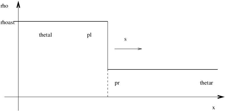
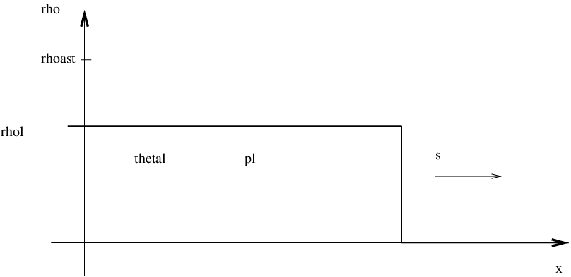
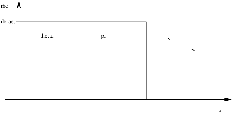
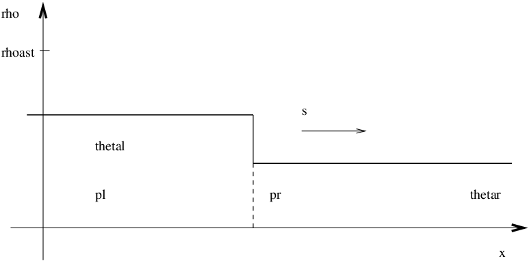
We note that (C)-(UC) interfaces or contact discontinuities (UC)-(UC) may incorporate a flip of the sign of $\theta$ in the velocity jump. This has no influence on the boundary values of $\bar{p}$ at the cluster boundary which is the quantity we wish to determine by this analysis. The Formal Statement 1 is illustrated in figure 4.

We now focus on the interface (C)-(C), i.e. a collision of two clusters. The procedure using limits $\varepsilon\rightarrow 0$ of the Riemann problem does not lead to any conclusion since the pressure becomes infinite. Note that this is also the case when dealing with the same limit in the standard Euler problem. Therefore, we have to find another strategy than using the Riemann problem. We turn our attention to the collision between two clusters of finite size and we show that the pressure involves a Dirac delta at the time of the collision. Such an analysis is inspired by the sticky block solutions presented in [10].

Consider two one-dimensional clusters which collide at a time $t_{c}$ (see fig. 5). Before collision, the left (resp. right) cluster at time $t<t_{c}$ extends between $a_{\ell}(t)$ and $b_{\ell}(t)$ (resp. $a_{r}(t)$ and $b_{r}(t)$) and moves with speed

$$\cos\theta_{\ell}=a_{\ell}^{\prime}(t)=b_{\ell}^{\prime}(t)\quad\text{(resp.}\ \cos\theta_{r}=a_{r}^{\prime}(t)=b_{r}^{\prime}(t)\text{)},$$

(2.41)

After the collision, the two clusters agregate and form a new cluster at time $t>t_{c}$ extending between $a(t)$ and $b(t)$ and moving with speed $\cos\theta=a^{\prime}(t)=b^{\prime}(t)$. Therfore, $\rho$ and $\theta$ are given for $t<t_{c}$ by

$$\rho=\rho^{\ast}\mathds{1}_{[a_{\ell}(t),b_{\ell}(t)]}+\rho^{\ast}\mathds{1}_{[a_{r}(t),b_{r}(t)]},\quad\theta=\theta_{\ell}\mathds{1}_{[a_{\ell}(t),b_{\ell}(t)]}+\theta_{r}\mathds{1}_{[a_{r}(t),b_{r}(t)]},$$

and for $t>t_{c}$ by

$$\rho=\rho^{\ast}\mathds{1}_{[a(t),b(t)]},\quad\theta=\theta\mathds{1}_{[a(t),b(t)]}.$$

where $\mathds{1}_{I}$ denotes the indicator function of the interval $I$ (i.e. $\mathds{1}_{I}(x)=1$ if $x\in I$ and $0$ otherwise). We denote by $m=b_{\ell}(t_{c})=a_{r}(t_{c})$ the collision point. We look for a pressure written as $\bar{p}(x,t)=\pi(x)\delta(t-t_{c})$. The following proposition provides conditions for such type of solutions to exist.

The proof of this proposition is developed in appendix C.

The underdetermined problem (2.12)-(2.15) must be complemented with the Formal Statement 1 which determines the boundary values of $\bar{p}$ at cluster boundaries and by proposition 2.3 which determines the evolution of two clusters when they meet. Strictly speaking, proposition 2.3 only gives the collision dynamics of two clusters in dimension 1. In dimension 2, clusters may have complicated shapes. So, the collision dynamics of two clusters in dimension 2 is a complicated problem which will be examined in a future work. At the present stage, problem (2.12)-(2.15) complemented with statement 1 fully determines the dynamics of the limit system as long as two clusters do not meet.

A rigorous theory of the well-posedness of system (2.12)-(2.15) complemented with statement 1 is outside the scope of the present paper. Let us just mention how a time discretized version of the problem can be computed. Suppose that $\rho^{n}(x)$, $\Omega^{n}(x)$, $\bar{p}^{n}(x)$ are approximations of $\rho(x,t^{n})$, $\Omega(x,t^{n})$, $\bar{p}(x,t^{n})$ at time $t^{n}=n\Delta t$. We solve the implicit system

	$\displaystyle\frac{\rho^{n+1}-\rho^{n}}{\Delta t}+\nabla_{\vec{x}}\cdot(\rho^{n+1}\Omega^{n+1})=0,$		(2.47)
	$\displaystyle\frac{\Omega^{n+1}-\Omega^{n}}{\Delta t}+(\Omega^{n}\cdot\nabla_{\vec{x}})\Omega^{n+\frac{1}{2}}+(\mbox{Id}-\Omega^{n+\frac{1}{2}}\otimes\Omega^{n+\frac{1}{2}})\nabla_{\vec{x}}\bar{p}^{n+1}=0,$		(2.48)

with

$$\Omega^{n+\frac{1}{2}}=\frac{\Omega^{n}+\Omega^{n+1}}{|\Omega^{n}+\Omega^{n+1}|}.$$

(2.49)

This form guarantees that $|\Omega^{n+1}|^{2}=|\Omega^{n}|^{2}=1$ (by taking the dot product by $\Omega^{n+\frac{1}{2}}$ and using that $|\Omega^{n+\frac{1}{2}}|=1$). $\bar{p}^{n+1}$ is determined by solving the elliptic equation

$$-\nabla_{\vec{x}}\cdot((\mbox{Id}-\Omega^{n+\frac{1}{2}}\otimes\Omega^{n+\frac{1}{2}})\nabla_{\vec{x}}\bar{p}^{n+1})=\nabla_{\vec{x}}\cdot((\Omega^{n}\cdot\nabla_{\vec{x}})\Omega^{n+\frac{1}{2}}).$$

(2.50)

on every connected component of the cluster region defined at time $t$ by $\{x\in{\mathbb{R}}^{2}\,|\,\rho^{n+1}(x,t)=\rho^{\ast}\}$. This equation must be supplemented with suitable boundary conditions on $\bar{p}$ at the boundary of the cluster. These boundary conditions are actually given by the Formal Statement 1, with right-hand sides evaluated at time $t^{n+1}$. The resolution of this equation guarantees that $\nabla\cdot\Omega^{n+1}=0$ on every connected component of a cluster, and shows that $\rho^{n+1}=\rho^{n}=\rho^{\ast}$ on such a cluster. Of course, the implicitness of the discretization leads to a nonlinear stationary problem, and the question of the existence of solutions for such a problem is not clear. However, intuitively, it seems that the prescription of the boundary values of $\bar{p}$ at cluster boundaries through the Formal Statement 1 leads to a well-posed problem, at least as long as two clusters do not meet.

To find out jump relations satisfied by the solutions of the system (2.12)-(2.15), the strategy is to solve the Riemann problem of the one-dimensional perturbation system (2.33)-(2.34) and to take the limit $\varepsilon\rightarrow 0$ of its solutions. This strategy was successfully adopted for a model of traffic jams in [6].

We note that the eigenvalues and eigenvectors of the hyperbolic system (2.33)-(2.34) are

$$\lambda_{\pm}^{\varepsilon}(\rho,\theta)=\cos\theta\pm\sqrt{\varepsilon p^{\prime}(\rho)\rho}|\sin\theta|,\quad\vec{r}_{\pm}^{\varepsilon}(\rho,\theta)=\left(\begin{array}[]{c}\pm\rho|\sin\theta|\\ \sqrt{\varepsilon p^{\prime}(\rho)\rho}\end{array}\right).$$

(3.51)

In this conservative system, the domain of $\theta$ is restricted to the interval $]0,\pi[$. But this is not a problem since our main concern is to find the missing conditions on $\bar{p}$ at the cluster boundary, and these only depend on jump conditions as functions of $\cos\theta$.

References

- [1] Aoki, I.: A simulation study on the schooling mechanism in fish. Bulletin of the Japanese Society of Scientific Fisheries (Japan) 48, 1081–1088 (1982)
- [2] Armbruster, D., Degond, P., Ringhofer, C.: Continuum models for interacting machines. Arch. Ration. Mech. Anal. 187(2), 185–220 (2008)
- [3] Ballerini, M., Cabibbo, N., Candelier, R., Cavagna, A., Cisbani, E., Giardina, I., Lecomte, V., Orlandi, A., Parisi, G., Procaccini, A., et al.: Interaction ruling animal collective behavior depends on topological rather than metric distance: Evidence from a field study. Proc. Nat. Acad. Sci. USA 105(4), 1232 (2008)
- [4] Barrat, A., Trizac, E., Ernst, M.: Granular gases: dynamics and collective effects. J. Phys. Condens. Matter 17(24), S2429 (2005)
- [5] Bellomo, N., Dogbe, C.: On the modelling crowd dynamics from scaling to hyperbolic macroscopic models. Math. Models Methods Appl. Sci. 18, 1317–1345 (2008)
- [6] Berthelin, F., Degond, P., Delitala, M., Rascle, M.: A model for the formation and the evolution of traffic jams. Arch. Rational Mech. Anal. 187(2), 185–220 (2008)
- [7] Berthelin, F., Degond, P., Le Blanc, V., Moutari, S., Rascle, M., Royer, J.: A traffic-flow model with constraints for the modeling of traffic jams. Math. Models Methods Appl. Sci 18, 1269–1298 (2008)
- [8] Bertin, E., Droz, M., Grégoire, G.: Boltzmann and hydrodynamic description for self-propelled particles. Phys. Rev. E. 74, 022,101 (2006)
- [9] Bouchut, F.: On zero pressure gas dynamics. Advances in kinetic theory and computing: selected papers, Ser. Adv. Math. Appl. Sci. 22, 171–190 (1994)
- [10] Bouchut, F., Brenier, Y., Cortes, J., Ripoll, J.F.: A hierarchy of models for two-phase flows. J. Nonlinear Sci. 10(6), 639–660 (2000)
- [11] Carrillo, J., D’Orsogna, M., Panferov, V.: Double milling in self-propelled swarms from kinetic theory. Kinet. Relat. Models 2(2), 363 – 378 (2009)
- [12] Carrillo, J., Fornasier, M., Rosado, J., Toscani, G.: Asymptotic flocking dynamics for the kinetic cucker-smale model. preprint (2009)
- [13] Cercignani, C., Illner, R., Pulvirenti, M.: The mathematical theory of dilute gases. Springer (1994)
- [14] Chuang, Y., Orsogna, M.D., Marthaler, D., Bertozzi, A., Chayes, L.: State transitions and the continuum limit for a 2D interacting, self-propelled particle system. Physica D: Nonlinear Phenomena 232(1), 33–47 (2007)
- [15] Couzin, I., Krause, J.: Self-organization and collective behavior in vertebrates. Advances in the Study of Behavior 32(1) (2003)
- [16] Couzin, I., Krause, J., James, R., Ruxton, G., Franks, N.: Collective memory and spatial sorting in animal groups. J. Theoret. Biol. 218(1), 1–11 (2002)
- [17] Cucker, F., Smale, S.: Emergent behavior in flocks. IEEE Trans. Automat. Control 52(5), 852–862 (2007)
- [18] Cucker, F., Smale, S.: On the mathematics of emergence. Japanese Journal of Mathematics 2(1), 197–227 (2007)
- [19] Degond, P.: Macroscopic limits of the Boltzmann equation: a review. Modeling and computational methods for kinetic equations, P. Degond, L. Pareschi, G. Russo (eds), Modeling and Simulation in Science, Engineering and Technology Series, Birkhauser, pp. 3–57 (2003)
- [20] Degond, P., Delitala, M.: Modelling and simulation of vehicular traffic jam formation. Kinet. Relat. Models 1, 279–293 (2008)
- [21] Degond, P., Motsch, S.: Continuum limit of self-driven particles with orientation interaction. Math. Models Methods Appl. Sci. 18, 1193–1215 (2008)
- [22] Degond, P., Motsch, S.: Large scale dynamics of the Persistent Turning Angle model for fish behaviour. J.Stat.Phys. 131(6), 989–1021 (2008)
- [23] D’Orsogna, M., Chuang, Y., Bertozzi, A., Chayes, L.: Self-propelled particles with soft-core interactions: patterns, stability, and collapse. Phys. Rev. Lett. 96(10), 104,302 (2006)
- [24] Gautrais, J., Jost, C., Soria, M., Campo, A., Motsch, S., Fournier, R., Blanco, S., Theraulaz, G.: Analyzing fish movement as a persistent turning walker. J. Math. Biol. 58(3), 429–445 (2008)
- [25] Gr´egoire G.and Chat´e, H.: Onset of collective and cohesive motion. Phys. Rev. Lett. 92, 025,702 (2004)
- [26] Ha, S.Y., Tadmor, E.: From particle to kinetic and hydrodynamic descriptions of flocking. Kinet. Relat. Models 1(3), 415–435 (2008)
- [27] Helbing, D.: Traffic and related self-driven many-particle systems. Rev. Modern Phys. 73(4), 1067–1141 (2001)
- [28] Helbing, D., Molnar, P.: Social force model for pedestrian dynamics. Math. Comput. Simul Phys Rev E 51, 4282–4286 (1985)
- [29] Maury, B., Venel, J.: A mathematical framework for a crowd motion model. C. R. Acad. Sci. Paris, Ser I 346(23-24), 1245–1250 (2008)
- [30] Maury, B., Venel, J.: Handling of contacts in crowd motion simulations. Trafic and Granular Flow ’07 (Springer, 2009. To appear)
- [31] Mogilner, A., Edelstein-Keshet, L.: A non-local model for a swarm. J. Math. Biol. 38(6), 534–570 (1999)
- [32] Mogilner, A., Edelstein-Keshet, L., Bent, L., Spiros, A.: Mutual interactions, potentials, and individual distance in a social aggregation. J. Math. Biol. 47(4), 353–389 (2003)
- [33] Moussaid, M., Garnier, S., Theraulaz, G., Helbing, D.: Collective information processing and pattern formation in swarms, flocks and crowds. Topics in Cognitive Science (2009)
- [34] Moussaid, M., Helbing, D., Garnier, S., Johansson, A., Combe, M., Theraulaz, G.: Experimental study of the behavioural mechanisms underlying self-organization in human crowds. Proc. R. Soc. Ser. B: Biological Sciences (2009, Published online)
- [35] Peruani, F., Deutsch, A., Bär, M.: Nonequilibrium clustering of self-propelled rods. Phys. Rev. E 74(3), 30,904 (2006)
- [36] Pillot, M.: Etude et modélisation des déplacements collectifs spontanés chez le mouton mérinos d’Arles (ovis aries). Master thesis (2006)
- [37] Pillot, M.H., Gautrais, J., Gouello, J., Michelena, P., Sibbald, A., Bon, R.: Moving together, incidental leaders and naïve followers (in prep.)
- [38] Poschel, T., Herrmann, H.: Size segregation and convection. Europhys. Lett. 29(2), 123–128 (1995)
- [39] Reynolds, C.: Flocks, herds and schools: A distributed behavioral model. In: Proceedings of the 14th annual conference on Computer graphics and interactive techniques, pp. 25–34. ACM New York, NY, USA (1987)
- [40] Serre, D.: Systems of Conservation Laws. Cambridge University Press (1999)
- [41] Slepcev, D.: Coarsening in nonlocal interfacial systems. SIAM J. Math. Anal. 40, 1029–1048 (2008)
- [42] Spohn, H.: Large Scale Dynamics of Interacting Particles. Springer-Verlag New York (1991)
- [43] Topaz, C., Bertozzi, A., Lewis, M.: A Nonlocal Continuum Model for Biological Aggregation. Bull. Math. Biol. 68(7), 1601–1623 (2006)
- [44] Vicsek, T., Czirók, A., Ben-Jacob, E., Cohen, I., Shochet, O.: Novel Type of Phase Transition in a System of Self-Driven Particles. Physical Review Letters 75(6), 1226–1229 (1995)