Thawing $f(R)$ cosmology

One of the proposals for explaining the present accelerated expansion of the universe [1] is modifying Einstein’s theory of gravity by introducing corrections to the Einstein-Hilbert lagrangian. These theories, called ”modified gravity theories” [2] follow this idea that the accelerated expansion of the universe may be has a geometric interpretation instead of adding the exotic forms of energy sources, dubbed ”dark energy” [3]. In the other words, in this perspective the dark energy is a manifestation of a modified gravitational interaction rather than a new form of energy density. The situation is reminiscent of the problem of precession of Mercury’s orbit. In the mid-nineteenth century the anomalous behavior of Mercury firstly was attributed to some unobserved (”dark”) planet in the solar system while it was mainly due to the failure of Newton’s theory of gravity in the strong gravitational field regime. In this view, it seems that as long as the dark energy particles [4] have not been observed directly, the ”geometric” candidates have important role. The simplest form of the modified gravity theories can be obtained by replacing the Ricci scalar $R$ with an arbitrary general function $f(R)$ in the Einstein-Hilbert action, usually called $f(R)$ theory of gravity. For a recent review of this theory see [5].

Metric $f(R)$ gravity model is dynamically equivalent to a BD scalar tensor theory with coupling constant $\omega=0$ [6]. By using this equivalence, one can easily find the prediction of metric $f(R)$ gravity for the PPN parameter $\gamma_{PPN}$. This parameter in the BD theory has the form $\gamma_{PPN}=(1+\omega)/(2+\omega)$. Thus the value of this parameter in the metric $f(R)$ gravity is $1/2$ which it is not in agreement with the experimental bound $|\gamma_{PPN}-1|<2.3:10^{-5}$[7]. However, considering this model in the Einstein frame has some satisfactory features. For example, $f(R)$ gravity can display the chameleon behavior in this frame which helps to relax the weak field limit problem of $f(R)$ gravity [8]. Chameleon effect is firstly interpreted using the scalar tensor framework of dark energy [9]. In this theory the effective mass of the scalar field is a function of the curvature of space-time and consequently it can be large at the solar system and small on the cosmological scales. This behavior appears in the minimally coupled scalar tensor theory if there exists an energy transfer between the dark energy fluid and the ordinary matter fluid. Since the quintessence model [10] is a minimally coupled scalar tensor theory, the chameleon mechanism can be appeared. On the other hand, metric $f(R)$ gravity theories are conformally equivalent to models of quintessence in which matter is coupled to the dark energy, thus the chameleon effect can occur in the conformal frame [8].

The noninteracting quintessence models can be divided into two categories [11]. ”Freezing” models: in these models the equation of state parameter of dark energy, $\omega_{\varphi}$, has an arbitrary value initially and decreases with time and asymptotically approaches $-1$. ”Thawing” models: these models have a value of $\omega_{\varphi}\sim-1$ initially, and it increases with time. There is a subset of freezing models which display tracking behavior [12]. In the tracking models, $\omega_{\varphi}$ has an arbitrary value initially and it is nearly constant during the tracking era. When the tracking era terminates then $\omega_{\varphi}$ decreases and asymptotically approaches -1. The important feature of these models is that the evolution of the scalar field is insensitive to the initial conditions and the dark energy density drops with a slower rate than the matter energy density and finally overtakes it. Albeit, these models can not provide a solution to the so-called coincidence problem because other fine-tunings are needed on the free parameters of these models in order to have an appropriate amount of dark energy compatible with observation in the present days[13].

In our recent paper[14] we derived some conditions for existing the stable tracker solutions in the Einstein frame of metric $f(R)$ gravity models. It is found that the tracker solutions with $-0.361<\omega_{\varphi}<1$ exist if $0<\Gamma<0.217$ and $\frac{d}{dt}\ln f^{\prime}(\tilde{R})>0$, where $\Gamma$ is a dimensionless function defined by relation (11) in the next section. The main purpose of this paper is to find out the necessary conditions for the existence of thawing behavior in the Einstein frame of metric $f(R)$ gravity theories.

The outline of this paper is as follows: In section II we start with BD scalar tensor theory (with an arbitrary $\omega$). As mentioned before, this theory behaves as an interacting quintessence model in this frame. We derive some necessary conditions on the form of the potential $V(\varphi)$ in order to lead to the thawing behavior for $\omega_{\varphi}$. In section III, by setting $\omega=0$ in the results, we present a general description of the behavior of the thawing $f(R)$ in the Einstein frame and finally conditions on the form of $f(R)$ gravity have been derived. Throughout this work we have chosen the unit $8\pi G=c=1$, the metric signature is $(+---)$ and the universe is assumed to be spatially flat.

The effective action for BD scalar tensor theory is given by

$$S_{J}=\int\sqrt{-\tilde{g}}\ d^{4}x\ [\Phi\tilde{R}-\frac{\omega}{\Phi}\Phi^{,\mu}\Phi_{,\mu}-2U(\Phi)+\mathcal{L}_{m}(\tilde{g}_{\mu\nu})]$$

(1)

where $\tilde{R}$ is the Ricci scalar, $U(\Phi)$ is the potential of the scalar field and $\mathcal{L}_{m}(\tilde{g}_{\mu\nu})$ represents the matter lagrangian density. Note that all tilded quantities are in the Jordan frame. The coupling constant $\omega$ should be large to pass the experimental testes. The observational constraint on $\omega$ is $|\omega|>40000$ [7]. Under the conformal transformation

$$g_{\mu\nu}=e^{\zeta\varphi}\tilde{g}_{\mu\nu}$$

(2)

where $\ln\Phi=\zeta\varphi$ and $\zeta=\sqrt{\frac{2}{3+2\omega}}$, one can obtain the Einstein frame action

$$\begin{split}S_{E}=\int\sqrt{-g}\ d^{4}x\ [R-\frac{1}{2}\varphi^{,\mu}&\varphi_{\mu}-V(\varphi)\\ &+\mathcal{L}_{m}(g_{\mu\nu}e^{-\zeta\varphi})]\end{split}$$

(3)

where $V(\varphi)=e^{-2\zeta\varphi}U(\Phi(\varphi))$. We see that in the Einstein frame the scalar field couples conformally to matter via the function $e^{-\zeta\varphi}$ but couples minimally to the gravity sector. For a spatially flat FRW universe, the modified Friedmann equations are given by

$$\begin{split}&H^{2}=\frac{1}{3}(\rho_{\varphi}+\rho_{m})\\ &\dot{H}=-\frac{1}{2}[(1+\omega_{m})\rho_{m}+(1+\omega_{\varphi})\rho_{\varphi}]\end{split}$$

(4)

and the equation of motion of the scalar field is

$$\ddot{\varphi}+3H\dot{\varphi}+V_{\varphi}=\sqrt{\frac{2}{3}}\beta(1-3\omega_{m})\rho_{m}$$

(5)

where $\beta=\sqrt{\frac{3}{8}}\ \zeta$, $\omega_{m}$ is the equation of state parameter of the ordinary matter with the energy density $\rho_{m}$ in the Einstein frame. Also $\rho_{\varphi}=\frac{1}{2}\dot{\varphi}^{2}+V(\varphi)$ and $p_{\varphi}=\frac{1}{2}\dot{\varphi}^{2}-V(\varphi)$ represent the energy density and pressure of the dark energy respectively. The conservation equations of the scalar field fluid and the cosmic fluid are

$$\begin{split}&\dot{\rho}_{\varphi}+3H(1+\omega_{\varphi})\rho_{\varphi}=\sqrt{\frac{2}{3}}\beta\dot{\varphi}(1-3\omega_{m})\rho_{m}\\ &\dot{\rho}_{m}+3H(1+\omega_{m})\rho_{m}=-\sqrt{\frac{2}{3}}\beta\dot{\varphi}(1-3\omega_{m})\rho_{m}\end{split}$$

(6)

and the energy density of matter $\rho_{m}$, pressure $p_{m}$, cosmic time $t$ and the scale factor $a$ are related to their Jordan frame counterparts through [15]

$\displaystyle\rho_{m}=e^{-2\zeta\varphi}\tilde{\rho}_{m},p_{m}=e^{-2\zeta\varphi}\tilde{p}_{m},dt=e^{\frac{\zeta\varphi}{2}}d\tilde{t},a=e^{\frac{\zeta\varphi}{2}}\tilde{a}$

(7)

During the matter dominated era, by using equation (5), one can introduce an effective potential as follows

$\displaystyle V_{eff}(\varphi)=V(\varphi)+\rho^{*}e^{-\sqrt{\frac{2}{3}}\beta\varphi}$

(8)

Where $\rho^{*}$ is a conserved quantity in the Einstein frame [9], which is related to $\rho_{m}$ via the relation $\rho_{m}=\rho^{*}e^{-\sqrt{\frac{2}{3}}\beta\varphi}$.

Since the late time evolution of the universe is of interest here and also our main purpose is to explore the role of the interaction term (which is nonzero for the matter component), we neglect the radiation component and assume that the universe contains only dust and dark energy. It is interesting to note that the interaction term is commonly assumed to be zero in the radiation dominated era, but recently Cembranos and et al [16] have shown that this interaction term can lead to strong impact on cosmology in the radiation dominated era due to the finite temperature radiative corrections. In the other words, there exists another source term for scalar field given by the conformal anomaly which leads to a nonzero trace of energy momentum tensor in the radiation dominated era (note that the RHS of (5) is the trace of energy momentum tensor). Considering the conformally coupled scalar field with a quadratic coupling function and vanishing potential, the above effect leads to a temporary contracting phase in which the temperature increases[16]. However, as mentioned before, we aim to study here the late time evolution of the universe and so we assume that the universe is filled with non-relativistic matter.

Following reference [17], we introduce the variables $x$, $y$ and $\lambda$ defined by

$\displaystyle x=\frac{\varphi^{\prime}}{\sqrt{6}},\ \ \ y=\sqrt{\frac{V(\varphi)}{3H^{2}}},\ \ \ \lambda=-\frac{V_{\varphi}}{V}$

(9)

where the prime denotes the derivative with respect to $\ln a$. By these definitions, it is an easy job to show that the equations (4) and (5) become

$\displaystyle\begin{split}&x^{\prime}=-3x+\lambda\sqrt{\frac{3}{2}}y^{2}+\frac{3}{2}x(1+x^{2}-y^{2})+\beta(1-x^{2}-y^{2})\\ &y^{\prime}=-\lambda\sqrt{\frac{3}{2}}xy+\frac{3}{2}y(1+x^{2}-y^{2})\\ &\lambda^{\prime}=-\sqrt{6}\lambda^{2}(\Gamma-1)x\end{split}$

(10)

where

$\displaystyle\Gamma=V\frac{d^{2}V}{d\varphi^{2}}/(\frac{dV}{d\varphi})^{2}$

(11)

For thawing models $\omega_{\varphi}\sim-1$ and so $\gamma=1+\omega_{\varphi}\ll 1$. Thus it is convenient to express the above equations with respect to $\gamma$ in order to exploit its smallness by expanding quantities to the lowest order in $\gamma$. Also we assume that $\dot{\varphi}>0$ $(x^{\prime}>0)$. This assumption, as considered in [14], is necessary to have an increasing dark energy density parameter i.e. $\dot{\Omega}_{\varphi}>0$. However, the results can be generalized to the opposite case $(x^{\prime}<0)$. Now, by using $\Omega_{\varphi}=x^{2}+y^{2}$ and $\gamma=2x^{2}/\Omega_{\varphi}$, one can rewrite the equations (10) in terms of $\gamma$ and $\Omega_{\varphi}$ as

$\displaystyle\gamma^{\prime}=(2-\gamma)\left(-3\gamma+\lambda\sqrt{3\gamma\Omega_{\varphi}}+\sqrt{\frac{2\gamma}{\Omega_{\varphi}}}\beta(1-\Omega_{\varphi})\right)$

(12)

$\displaystyle\Omega_{\varphi}^{\prime}=3(1-\Omega_{\varphi})\left((1-\gamma)\Omega_{\varphi}+\frac{\beta}{3}\sqrt{2\gamma\Omega_{\varphi}}\right)$

(13)

$\displaystyle\lambda^{\prime}=-\sqrt{3}\lambda^{2}(\Gamma-1)\sqrt{\gamma\Omega_{\varphi}}$

(14)

It is clear from equation (13) that for thawing models $\Omega^{\prime}_{\varphi}\neq 0$ during the cosmological history of the universe $(0<\Omega_{\varphi}<1)$. Thus by using (13) we can write equation (12) as follows

$\displaystyle\frac{d\gamma}{d\Omega_{\varphi}}=\frac{(2-\gamma)\left(-3\gamma+\lambda\sqrt{3\gamma\Omega_{\varphi}}+\sqrt{\frac{2\gamma}{\Omega_{\varphi}}}\beta(1-\Omega_{\varphi})\right)}{3\Omega_{\varphi}(1-\Omega_{\varphi})\left(1-\gamma+\frac{\beta}{3}\sqrt{\frac{2\gamma}{\Omega_{\varphi}}}\right)}$

(15)

This equation is obtained earlier in [18] in which, the non-minimal quintessence with nearly flat potentials has been considered. Equation (15) is not a simple differential equation and for solving it, we will make some assumptions which are satisfied for thawing models. First assume that $\gamma\ll 1$, by retaining terms up to the first order in $\gamma$, the equation (15) takes the following form

$\displaystyle\begin{split}\frac{d\gamma}{d\Omega_{\varphi}}&\simeq\frac{-2\gamma}{\Omega_{\varphi}(1-\Omega_{\varphi})}-\sqrt{\frac{8}{21}}\beta\frac{\lambda\gamma}{\Omega_{\varphi}(1-\Omega_{\varphi})}\\ &+\frac{2\lambda\sqrt{\gamma}}{\sqrt{3\Omega_{\varphi}}(1-\Omega_{\varphi})}+\frac{2\beta\sqrt{2\gamma}}{3\Omega_{\varphi}^{3/2}}-\frac{4\beta^{2}\gamma}{9\Omega_{\varphi}^{2}}\end{split}$

(16)

Another useful equation can be obtained by using the equation of motion of the scalar field (5)

$\displaystyle\lambda=\sqrt{\frac{3\gamma}{\Omega_{\varphi}}}[1+\frac{\gamma^{\prime}}{3\gamma(2-\gamma)}]-\frac{\sqrt{\frac{8}{3}}\beta}{2-\gamma}\frac{1-\Omega_{\varphi}}{\Omega_{\varphi}}$

(17)

This equation can be written to the first order in $\gamma$ as follows

$$\lambda\simeq\left[\sqrt{\frac{3\gamma}{\Omega_{\varphi}}}(1+\frac{\gamma^{\prime}}{6\gamma})-\sqrt{\frac{1}{6}}\beta\gamma\frac{1-\Omega_{\varphi}}{\Omega_{\varphi}}\right]-\sqrt{\frac{2}{3}}\beta\frac{1-\Omega_{\varphi}}{\Omega_{\varphi}}$$

(18)

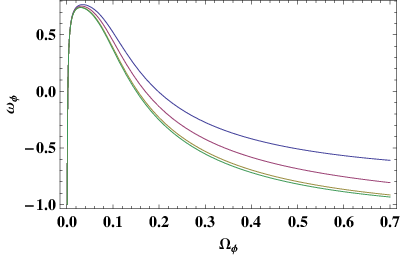
For uncoupled quintessence, where $\beta$ is zero, the RHS of equation (17) is approximately constant and moreover it has an small amount (note that $\gamma\ll 1$) for thawing solutions . Thus if $(\frac{V_{\varphi}}{V})^{2}\ll 1$ then the thawing behavior can occur [19]. In the general case where $\beta$ is not zero, then the RHS can not be regarded as a constant. Since $\Omega_{\varphi}$ is appeared in the denominator, hence the second term in the RHS is dominated initially and has a large value. Thus the LHS can not have a small value as well as can not be a constant. When $\Omega_{\varphi}$ gets larger, the effect of the interaction becomes weaker. Thus, at late times, the nearly flat region of the potential leads to the thawing uncoupled quintessence. So, unlike the noninteracting quintessence model, nearly flat potentials can not lead to the thawing behavior when an explicit energy transfer between the scalar field fluid and the matter fluid exists. In this case, as mentioned in [18], with nearly flat potentials, $\omega_{\varphi}$ firstly increases with time and then, when the interaction becomes weaker, it decreases and approaches asymptotically to a value near $-1$. The behavior of $\omega_{\varphi}$ with nearly flat potentials has been plotted in Fig.1 by solving equation (15) numerically. Note that this behavior is due to the special form of interaction which appeared here (i.e. $\dot{\varphi}\rho_{m}$).

Now we are ready to make the second assumption. Taking into account equation (18) and assuming that the value of the term within the bracket to be approximately constant for thawing solutions, this equation gives

$$\lambda\simeq\lambda_{0}-\sqrt{\frac{2}{3}}\beta\frac{\rho_{m}}{\rho_{\varphi}}=\lambda_{0}-\sqrt{\frac{2}{3}}\beta\frac{1-\Omega_{\varphi}}{\Omega_{\varphi}}$$

(19)

where $\lambda_{0}$ is a positive constant. Hereafter we shall refer to this equation as the ”thawing condition”. For potentials in which $-\frac{V_{\varphi}}{V}$ decreases as $\varphi$ increases ($\Gamma>1$), the LHS of the equation (19) is increasing. On the other hand, the RHS is increasing because $\Omega_{\varphi}$ increases. Hence, the thawing condition can not be satisfied. Thus, the thawing condition shows that it is necessary $\lambda$ increases with time when $\varphi$ and $\Omega_{\varphi}$ are increasing, i.e.

$$\Gamma<1$$

(20)

It is clear from the thawing condition that if $\beta=0$ then $\lambda$ is nearly constant and so $\Gamma\simeq 1$. One can find other simple conditions on the form of $V(\varphi)$ by using the thawing condition. For this purpose, let us rewrite (19) as follows

$$\frac{1}{V}\frac{dV}{d\varphi}\simeq-(\lambda_{0}+\sqrt{\frac{2}{3}}\beta)+\sqrt{\frac{2}{3}}\beta\frac{1}{\Omega_{\varphi}}$$

(21)

It is clear from this equation that the second term in the RHS is dominated initially and so $\frac{dV}{d\varphi}>0$. As mentioned before, the interaction becomes weaker at late times. Thus, there exists a time $t^{*}$, at which

$$\left(\lambda_{0}+\sqrt{\frac{2}{3}}\beta\right)_{t=t^{*}}\simeq\sqrt{\frac{2}{3}}\beta\left(\frac{1}{\Omega_{\varphi}}\right)_{t=t^{*}}$$

(22)

At this time $\frac{dV}{d\varphi}\simeq 0$ and after it $\frac{dV}{d\varphi}<0$. Thus, it is necessary that the potential has a maximum in order to have thawing behavior. In the other words, a value of the scalar field, $\varphi^{*}$ should exist such that

$$\begin{split}&\frac{dV}{d\varphi}|_{\varphi^{*}}=0\\ &\frac{d^{2}V}{d\varphi^{2}}|_{\varphi^{*}}<0\end{split}$$

(23)

Now let us to justify the thawing condition. By these assumptions ($\gamma\ll 1$ and (19)), equation (16) takes the very simple following form

$\displaystyle\frac{d\gamma}{d\Omega_{\varphi}}+\frac{2A\gamma}{\Omega_{\varphi}(1-\Omega_{\varphi})}-\frac{2\lambda_{0}\sqrt{\gamma}}{\sqrt{3\Omega_{\varphi}}(1-\Omega_{\varphi})}\simeq 0$

(24)

in which $A=1+\beta\sqrt{\frac{2}{27}}\lambda_{0}$. Note that if $\beta=0$, then this equation becomes precisely the equation obtained earlier by Scherrer and Sen [19]. This differential equation has an exact solution as follows

$\displaystyle\begin{split}\gamma=\left(\frac{1-\Omega_{\varphi}}{\Omega_{\varphi}}\right)^{2A}[\ \chi_{0}+&\frac{2\lambda_{0}\Omega_{\varphi}^{1/2+A}}{\sqrt{3}(1+2A)}\ \\ &{}_{2}F_{1}(\frac{1}{2}+A,1+A,\frac{3}{2}+A,\Omega_{\varphi})\ ]^{2}\end{split}$

(25)

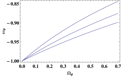
where $\chi_{0}$ is an integration constant depending on the initial conditions and ${}_{2}F_{1}$ is the Gauss Hypergeometric function. This equation gives an analytical expression for the state parameter of dark energy as a function of its density parameter for the thawing non-minimal quintessence model. It generalizes the result obtained in [19] for thawing minimally coupled scalar field. The behavior of $\omega_{\varphi}$ as a function of $\Omega_{\varphi}$ has been shown in Fig.2 for various values of $\lambda_{0}$. The $\beta$ has been chosen to be $0.5$, the value will be used in the next section in the case of $f(R)$ gravity models. In fact, the value of $\lambda_{0}$ should be such that $\omega_{\varphi}$ has a value near $-1$ today.

For confronting the model with observational data, it is needed to express $\gamma$ and $\Omega_{\varphi}$ in terms of cosmic red shift or cosmic scale factor. By substituting the solution (25) in the equation (13), we obtain a differential equation for $\Omega_{\varphi}$ in which the Gauss Hypergeometric function is appeared. Here, we have solved it numerically and the result has been compared with the exact solution of the equation (13) when $\gamma=0$, in Fig.3. Thus as it is clear from Fig.3, the difference between these solutions is small when $\lambda_{0}\sim 1$ and consequently one can use the solution of (13) when $\gamma=0$ i.e.

$$\Omega_{\varphi}=[1+(\Omega_{\varphi 0}^{-1}-1)a^{-3})]^{-1}$$

(26)

in order to find out an approximated expression for $\gamma$ as a function of $a$.

Now let us consider $f(\tilde{R})$ gravity in the Einstein frame. It is sufficient to set $\omega=0$ (and so $\zeta=\sqrt{\frac{2}{3}}$) in equation (25) in order to have thawing behavior in the Einstein frame. Also in the context of $f(\tilde{R})$ gravity, the scalar field $\varphi$ is related to the curvature scalar of the Jordan frame as follows

$$\begin{split}&\varphi=\sqrt{3/2}\ln f_{\tilde{R}}(\tilde{R})\\ &V(\varphi)=(\tilde{R}f_{\tilde{R}}-f)/2f_{\tilde{R}}^{2}\end{split}$$

(27)

where $f_{\tilde{R}}=\frac{df}{d\tilde{R}}$. As it is clear from Fig.2, $\lambda_{0}$ has been chosen near to $1$ in order to have $\omega_{\varphi}$ near $-0.9$. In this case, as it has been shown in Fig.3, $\Omega_{\varphi}$ evolves as the dark energy density parameter of $\Lambda$CDM model in which $\omega_{\varphi}$ is always approximated to $-1$.

Now, we want to find out explicit conditions on the form of the function $f(\tilde{R})$ in order to have thawing behavior in the Einstein frame. Taking into account equations (20) and (27), one can easily verify that if $f_{\tilde{R}\tilde{R}}>0$ then

$$\tilde{R}f_{\tilde{R}}^{2}-(\tilde{R}f_{\tilde{R}\tilde{R}}+f_{\tilde{R}})f<0$$

(28)

and for $f_{\tilde{R}\tilde{R}}<0$

$$\tilde{R}f_{\tilde{R}}^{2}-(\tilde{R}f_{\tilde{R}\tilde{R}}+f_{\tilde{R}})f>0$$

(29)

Also, by using (23) and (27), it is necessary that the form of $f(\tilde{R})$ be such that there exists $\tilde{R}^{*}$ for which

$$\begin{split}&\tilde{R}^{*}=\frac{2f}{f_{\tilde{R}}}|_{\tilde{R}^{*}}\\ &\tilde{R}^{*}>\frac{f_{\tilde{R}}}{f_{\tilde{R}\tilde{R}}}|_{\tilde{R}^{*}}\end{split}$$

(30)

Note that for having nonsingular conformal transformation (equations (27) and (2)) we have assumed $f_{\tilde{R}}>0$. Equations (28)-(30) are the necessary conditions on the form of $f(\tilde{R})$ for raising to the thawing behavior and they are not sufficient conditions.

Now, let us to find out an explicit example for thawing potentials. For this purpose, assume that

$$\frac{d\varphi}{d\Omega_{\varphi}}=\frac{\alpha}{1-\Omega_{\varphi}}$$

(31)

where, $\alpha$ is a positive constant. This assumption leads to the following form of dark energy density parameter

$$\Omega_{\varphi}=1-e^{-\frac{(\varphi-\psi)}{\alpha}}$$

(32)

which is an increasing function of $\varphi$ and $\psi$ is an integration constant. Using $\varphi^{\prime}=\sqrt{3\gamma\Omega_{\varphi}}$ and equations (13), (31) and (32), we obtain

$$\gamma=\frac{B+18\alpha^{2}\Omega_{\varphi}\mp\sqrt{B^{2}+36B\alpha^{2}\Omega_{\varphi}}}{18\alpha^{2}\Omega_{\varphi}}$$

(33)

where $B=3-2\sqrt{2}\alpha\beta+2\alpha^{2}\beta^{2}$. If $\alpha$ is a small quantity ($\alpha<1$), then the solution with minus sign can yield to the thawing behavior. For seeing this, $\omega_{\varphi}$ has been plotted in Fig.4 for various values of $\alpha$. By substituting equation (33) into equation (17) and expanding the RHS of equation (17) to the second order in $\alpha$ (note that we have assumed that $\alpha$ is small), we get

$$\frac{1}{V}\frac{dV}{d\Omega_{\varphi}}\approx\frac{-\sqrt{\frac{2}{3}}\beta}{\Omega_{\varphi}}\alpha+\frac{1+6\Omega_{\varphi}}{2(1-\Omega_{\varphi})}\alpha^{2}+O(\alpha^{3})$$

(34)

which has the following solution

$$V\approx V_{0}\Omega_{\varphi}^{\sqrt{\frac{2}{3}}\alpha\beta}(1-\Omega_{\varphi})^{\frac{7\alpha^{2}}{2}}e^{3\alpha^{2}\Omega_{\varphi}}$$

(35)

where $V_{0}$ is a positive integration constant. It is obvious from this that $V$ has a maximum and so it is consistent with our pervious results. By setting $\psi$ to be zero and using equation (32), let us rewrite equation (35) as a function of the scalar field as follows

$$V\approx V_{0}\ e^{-\frac{7\alpha}{2}\varphi}(1-e^{-\frac{\varphi}{\alpha}})^{\sqrt{\frac{2}{3}}\alpha\beta}e^{3\alpha^{2}(1-e^{-\frac{\varphi}{\alpha}})}$$

(36)

This potential satisfies the conditions (20) and (23) and it is a two parameter potential ($V_{0}$ and $\alpha$). The parameter $\alpha$ should be small and for $-1<\omega_{\varphi 0}<-0.9$ it should be $0<\alpha<0.23$. Thus, the only free parameter in this model is $V_{0}$. As mentioned before, this free parameter should be fin-tuned by using the observational data. The observational fact is that the energy density of dark energy and the energy density of cosmic matter fluid are approximately in the same order. Since the potential has been obtained with respect to $\Omega_{\varphi}$ (equation (35)) it is easy to make an estimation on the values of $V_{0}$ to reproduce the acceleration expansion. Albeit, we assume that the major contribution to the energy of the scalar field is due to the potential term (note that this is the case for all thawing potentials). The density parameter of dark energy is

$$\Omega_{\varphi}\sim\frac{V}{3H^{2}}$$

(37)

By using this equation and (35) we obtain

$$\frac{V_{0}}{3H_{0}^{2}}\sim\Omega_{\varphi 0}^{1-\sqrt{\frac{2}{3}}\alpha\beta}(1-\Omega_{\varphi 0})^{-\frac{7\alpha^{2}}{2}}e^{-3\alpha^{2}\Omega_{\varphi 0}}$$

(38)

where $H_{0}$ is the current value of the Hubble parameter. By taking into account that the current value of $\Omega_{\varphi 0}$ satisfies the bound $0.6\leq\Omega_{\varphi 0}\leq 0.8$, we have plotted the region of parameter space able to cover the above observational constraints, in Fig. 5. This region varies from $\alpha=0$ to $\alpha=0.23$ and from $\hat{V_{0}}\approx 0.6$ to $\hat{V_{0}}\approx 0.95$, where $\hat{V_{0}}$ is a dimensionless variable defined as follows

$$\hat{V_{0}}=\frac{V_{0}}{3H_{0}^{2}}$$

(39)

Note that for making a more precise estimation one should use numerical solutions of the field equations and taking into account the effect of the kinetic term of energy density of the dark energy, see the third paper of [13] and also [20] for more details.

Now, for finding the corresponding $f(\tilde{R})$ function, assume that $f(\tilde{R})$ differs from Einstein’s general relativity by a small perturbation as follows

$$f(\tilde{R})=\tilde{R}+\varepsilon\Psi(\tilde{R})$$

(40)

where $\varepsilon$ is a very small parameter. By substituting this in equation (27), using (36) and taking $\beta=0.5$, one reaches to the following first order differential equation up to the first order in $\varepsilon$

$$-\varepsilon\Psi(\tilde{R})+\varepsilon\Psi_{\tilde{R}}\approx 2V_{0}\left(\frac{3}{2}\right)^{\frac{\alpha}{2\sqrt{6}}}\left(\frac{\varepsilon\Psi_{\tilde{R}}}{\alpha}\right)^{\sqrt{\frac{1}{6}}\alpha}$$

(41)

which has the solution of the form

$$\varepsilon\Psi(\tilde{R})\approx-\mu\tilde{R}^{n}$$

(42)

where

$$\begin{split}&n=\frac{\alpha}{\alpha-\sqrt{6}}\\ &\mu=2V_{0}(1-\frac{\alpha}{\sqrt{6}})\left(\frac{12}{\sqrt{9^{\alpha}}V_{0}}\right)^{n}\ 3^{\frac{\alpha}{\sqrt{6}}}\end{split}$$

(43)

Since $\alpha$ is a positive constant, $n$ is a negative real number. Thus, the perturbation procedure is valid if the curvature of space time is sufficiently high such that $\left|-\mu\tilde{R}^{n}\right|\ll\tilde{R}$. Consequently, the model (42) can lead to the thawing behavior only in the beginning of matter dominated era. However, for larger values of $\varphi$, let us expand the potential (36) again. Before proceeding, we expect that $\Psi(\tilde{R})$ contains some terms of $\tilde{R}$ with powers smaller than $n$. Because such a term can have effect in the late times (large $\varphi$), where the curvature is small, while it can be neglected compared with $\tilde{R}^{n}$ where the curvature is larger.

If $\varphi$ is large enough such that $e^{-\frac{\varphi}{\alpha}}\ll 1$ then one can write the potential (36) as follows

$$V\approx V_{0}e^{3\alpha^{2}}\ e^{-\frac{7\alpha}{2}\varphi}$$

(44)

It is easy to show that the $f(\tilde{R})$ function corresponding to this potential is

$$f(\tilde{R})\sim\nu\tilde{R}^{m}$$

(45)

where

$$\begin{split}&m=\frac{7\sqrt{6}\alpha-8}{7\sqrt{6}\alpha-4}\\ &\nu=\frac{2V_{0}e^{3\alpha^{2}}(1-7/2\sqrt{3/2}\alpha)}{(2V_{0}e^{3\alpha^{2}}(2-7/2\sqrt{3/2}\alpha))^{m}}\end{split}$$

(46)

It is possible to make an estimation on the value of $\alpha$ by assuming that the potential (44) is a solution of differential equation (19) when $\Omega_{\varphi}\sim 1$. Thus, $\lambda_{0}\sim\frac{7}{2}\alpha$ and consequently $\alpha\sim\frac{2}{7}$. By this amount for $\alpha$, $m$ is negative and also it is smaller than $n$ (m= -3.45), as we expected.

As a result, the following model

$$f(\tilde{R})\sim\tilde{R}-\mu\tilde{R}^{n}+\nu\tilde{R}^{m}$$

(47)

can lead to the thawing behavior in the matter dominated epoch and late times. Note that this model satisfies the condition (20). Also, as we required, it’s corresponding potential in the Einstein frame has a maximum.

We have considered BD scalar tensor theory in the Einstein frame. In this frame, BD theory behaves like an interacting quintessence. It is necessary that the potential $V(\varphi)$ has a maximum in the region where the scalar field rolls in order to have thawing behavior. Also the potential should satisfy the condition $\Gamma<1$. The thawing condition (19) shows that for non-interacting quintessence model, potential should satisfy the condition $\Gamma\approx 1$ [19].

In the last section, by setting the BD coupling constant $\omega$ to zero, we have studied the thawing behavior of $f(\tilde{R})$ gravity models in the Einstein frame. It is important to note that for power law $f(\tilde{R})$ gravity models, such as (45), the equation of state parameter of dark energy (in the Einstein frame) firstly increases with time and then decreases. This behavior is due to the form of the corresponding potential of these models in the Einstein frame. For these models, $\lambda$ is constant and as we have mentioned in section II, $\omega_{\varphi}$ evolve as Fig. 1. The sign of the power of $\tilde{R}$ depends on the present day value of $\omega_{\varphi}$ and it’s magnitude depends on $\lambda_{0}$. As it is clear from Fig. 1, choosing different values for $\lambda_{0}$ leads to different values of $\omega_{\varphi}$ at the present day.

As an example for thawing $f(\tilde{R})$ models, we have proposed the model given by (47). The corresponding potential has a maximum and the condition $\Gamma<1$ is satisfied. So, in the beginning of the matter dominated era $\lambda$ is not approximately constant, (see equation (34)), and $\omega_{\varphi}$ increases slowly as it has been shown in Fig. 4. Also this model leads to a nearly flat potential in the late times which is satisfactory. At sufficiently late times, the interaction term in equation (17) is negligible and we expect our model behaves like a non-interacting thawing quintessence [19].

We would like to thank the referee for useful comments. M. Roshan would like to thanks J.A. Cembranos for useful hints and communications. This work is partly supported by a grant from university of Tehran and partly by a grant from center of excellence of department of physics on the structure of matter.

References

- [1] A.G. Riess and et al, Astron. J. 116,1009 (1998); V. Sahni and A.A. Staroboinsky, Int. J. Mod. Phys. D 9, 373 (2000); S.M. Carroll, Living Rev. Rel. 4, 1, (2001); T. Padmanabhan, Phys. Rept. 380, 235 (2003).
- [2] A.D. Dolgov and M. Kawasaki, Phys. Lett. B 573,1 (2003); A. Lue, R. Scoccimarro and G. Starkman, Phys. Rev. D 69, 044005 (2004); L. Amendola, D. Polarski and S. Tsujikawa, Phys. Rev. Lett. 98, 131302 (2007).
- [3] E.J. Copeland, M. Sami, S. Tsujikawa, Int . J. Mod. Phys. D 15,1753-1936 (2006);P.J.E. Peebles, B. Ratra, Rev. Mod. Phys. 75, 559-606 (2003).
- [4] M. L. Perl, arXiv: 0809.5083, 34th Int. Conf. on HEP, Piladelphia (2008);A. de la Macorra, Phys. Rev. D 72, 043508 (2005); S. DeDeo, Phys. Rev. D 73, 043520 (2006).
- [5] T.P. Sotiriou and V. Faraoni ,arXiv:0805.1726 (2008).
- [6] T.P. Sotiriou, Class. Quantum. Grav. 23, 5117 (2006).
- [7] B. Bertotti, L. Iess and P. Tortora, Nature 425, 374 (2003).
- [8] J.A.R. Cembranos, Phys. Rev. D 73, 064029 (2006); A.A. Starobinsky, JETP Lett. 86, 157 (2007); T. Fulkner, M. Tegmark, E.F. Bunn and Y. Mao, Phys. Rev. D 76, 063505 (2007).
- [9] J. Khoury and A. Weltman, Phys. Rev. D 69, 044026 (2004); J. Khoury and A. Weltman, Phys. Rev. Lett. 93, 171104 (2004).
- [10] C. Wetterich, Astron. Astrophys. 301, 321 (1995); B. Ratra and P.J.E. Peebles, Phys. Rev D 37, 3406 (1988); P.J.E. Peebles and B. Ratra, Astrophys. J. Lett. 325, L17 (1988); R.R. Caldwell, R. Dave, P.J. Steinhardt, Phys. Rev. Lett. 80, 1582 (1998).
- [11] R.R. Caldwell and E.V. Linder, Phys. Rev. Lett. 95, 141301 (2005).
- [12] P.J.Steinhardt, L. Wang and Ivaylo Zlatev, Phys. Rev. Lett. 82, 896-899 (1999); P.J. Steinhardt, L. Wang, I. Zlatev, Phys. Rev. D 59, 123504 (1999).
- [13] S. Weinberg, Cosmology (Oxford University Press, New York, 2008) Sec. 1.12, S.M. Carroll, AIP Conf. Proc. 743, 16 (2004), astro-ph/0310342; U. Franca, R. Rosenfeld, JHEP10 (2002) 015.
- [14] M. Roshan and F. Shojai, Phys. Rev. D 79, 103510 (2009).
- [15] V. Faraoni, Cosmology in scalar-tensor gravity (Kluwer Academic Publishers, Dordrecht, 2004)
- [16] J.A.R. Cembranos, K.A. Olive, M. Peloso and J.P. Uzan, arXiv:0905.1989.
- [17] E.J. Copeland, A.R. Liddle, and D. Wands, Phys. Rev. D 57, 4686 (1998). A. de la Macorra and G. Piccinelli, Phys. Rev. D 61, 123503 (2000); S.C.C. Ng, N.J. Nunes and F. Rosati, Phys. Rev. D 64, 083510 (2001).
- [18] A.A. Sen, G. Gupta and S. Das, arXiv:0901.0173 (2009)
- [19] R.J. Scherrer and A.A. Sen, Phys. Rev. D 77, 083515 (2008)
- [20] U. Franca, R. Rosenfeld, Phys. Rev. D 69, 063517 (2004)