跳到论文正文
W Papers独立论文阅读器 arXiv:0908.1684 论文正文 计算阅读时间 · 0%
引用这篇论文根据当前论文元数据生成,正式投稿前建议核对。


License: arXiv.org perpetual non-exclusive license
arXiv:0908.1684v1 [hep-ph] 12 Aug 2009

Renormalization of Twist-Four Operators in QCD

V.M. Braun a, A.N. Manashov a,b and J. Rohrwild a

aInstitut für Theoretische Physik, Universität Regensburg,
D-93040 Regensburg, Germany

bDepartment of Theoretical Physics, St.-Petersburg State University
199034, St.-Petersburg, Russia

Version of August 24, 2026

Abstract:

Extending the work by Bukhvostov, Frolov, Lipatov and Kuraev (BFLK) on the renormalization of quasipartonic operators we derive a complete set of two-particle renormalization group kernels that enter QCD evolution equations to twist-four accuracy. It is shown that the 2→22\to 2 evolution kernels which involve “non-partonic” components of field operators, and, most remarkably, also 2→32\to 3 kernels do not require independent calculation and can be restored from the known results for quasipartonic operators using conformal symmetry and Lorentz transformations. The kernels are presented for the renormalization of light-ray operators built of chiral fields in a particular basis such that the conformal symmetry is manifest. The results can easily be recast in momentum space, in the form of evolution equations for generalized parton distributions.

1 Introduction

Higher-twist effects generically correspond to corrections to hadronic observables that are suppressed by a power of the (large) momentum transfer or the heavy quark mass. One application where such effects are phenomenologically relevant are high precision studies of the total cross section of deep-inelastic lepton-hadron scattering (DIS). In this case the leading-twist calculations within the standard DGLAP formalism are advanced to the next-to-next-to-leading order. Also lattice calculations of the moments of parton distributions with an accuracy at a percent level are becoming feasible. In this situation taking into account twist-four corrections that are suppressed by a power of the photon virtuality Q2Q^{2} proves to be increasingly important for the analysis of modern data, see e.g. [1, 2, 3, 4, 5, 6]. Twist-three effects are actively discussed in the context of exclusive and semi-inclusive reactions, e.g. deeply-virtual Compton scattering [7, 8] and diffractive electroproduction of vector mesons [9], single spin asymmetry in various reactions [10, 11, 12, 13, 14, 15, 16], etc. One can expect that with the increasing accuracy of the experimental data the twist-four effects will start playing a role here as well. Another large field of applications are the studies of higher-twist hadron distribution amplitudes (e.g. [17, 18, 19, 20]) that provide one with the important input to the so-called light-cone sum rules [21, 22].

The theoretical description of higher-twist corrections is based on the Wilson Operator Product Expansion (OPE) and involves contributions of a large number of local operators. The corresponding leading-order coefficient functions are usually easy to calculate (e.g. twist-four contributions to DIS are known since many years [23, 24]) but the operator renormalization for the operators of twist-four and higher has not been studied systematically. Up to now, twist-four anomalous dimensions are only known for a subset of four-quark operators [25] and for a few quark-gluon operators of lowest dimension (e.g. [26, 27, 28, 29]). In addition, the structure of the most singular parts of the mixing kernels for small values of the Bjorken variable that are relevant for the contribution of two-pomeron cuts in high-energy scattering processes was considered in [30, 31].

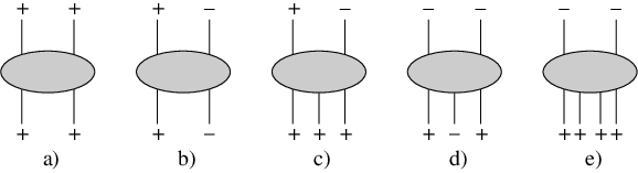
A general formalism was developed by Bukhvostov, Frolov, Lipatov and Kuraev (BFLK) [32] for the special class of so-called quasipartonic operators that are built of “plus” components of quark and gluon fields. For each twist, the set of quasipartonic operators is closed under renormalization and the renormalization group (RG) equation can be written in a Hamiltonian form that involves two-particle “interaction” kernels, cf. Fig. 1a, that can be expressed in terms of two-particle Casimir operators of the collinear subgroup S​L​(2,ℝ)SL(2,{\mathbb{R}}) of the conformal group. In this formulation symmetries of the RG equations become explicit. Moreover, the corresponding three-particle quantum-mechanical problem turns out to be completely integrable for a few important cases, and in fact reduces to a Heisenberg spin chain [33]. An almost complete understanding achieved at present of the renormalization of twist-three operators is due to all these formal developments, see [34, 35] for a review and further references.

The goal of our study is to generalize the BFLK approach to the situation where not all contributing operators are quasipartonic, as it proves to be the case starting with twist four. On this way, there are two complications.

First, the number of fields (“particles”) is not conserved. To one-loop accuracy, the mixing matrix of operators with a given twist has a block-triangular structure as the operators with less fields can mix with ones containing more fields but not vice versa. Operators with the maximum possible number of fields are quasipartonic.

Second, operators involving “minus” and “transverse” derivatives and/or field components must be included. The problem is that transverse derivatives generally do not have good transformation properties with respect to the S​L​(2,ℝ)SL(2,\mathbb{R}) group. In concrete applications it may be possible to get rid of such operators using equations of motion (EOM) and exploiting specific structure of the matrix elements of interest, e.g. if there is no transverse momentum transfer between the initial and the final state. The main problem as far as the operator renormalization is concerned is that after this reduction the conformal symmetry becomes obscured. In the work [36] we have suggested a different, general approach based on the construction of a complete conformal operator basis for all twists. In this basis, the S​L​(2,ℝ)SL(2,{\mathbb{R}}) symmetry of the RG equations is manifest.
Refer to caption

Figure 1: Schematic structure of one-loop renormalization group kernels in QCD

Another important observation was made in [37] where it was shown that the diagonal part of one-loop QCD RG equations (for arbitrary twist) can be written in a Hamiltonian form in terms of quadratic Casimir operators of the full conformal group S​O​(4,2)SO(4,2). This implies that the 2→22\to 2 kernels of the type shown in Fig. 1b can be obtained from the BFLK kernels in Fig. 1a by the corresponding replacement. Our first goal will be to work out the corresponding relations using the conformal basis of Ref. [36] for generic twist-four operators.

The main new contribution of this work is the calculation of 16 independent 2→32\to 3 kernels corresponding to operator mixing of one “partonic” and one “non-partonic” field in three-particle quasipartonic operators, shown schematically in Fig. 1c. To this end we suggest a new technique based on application of Lorentz transformations (translations and rotations in the transverse plane) to the “diagonal” 2→22\to 2 kernels, which bypasses calculation of Feynman diagrams.

Combining the kernels in Fig. 1a,b,c one obtains a complete set of building blocks for the renormalization of twist-4 operators that involve at most one “non-partonic” field. Strictly speaking, (two-particle) twist-4 operators containing two “non-partonic” fields also exist and have to be included. They can mix into three-particle and also four-particle operators as in Fig. 1d,e. However, contributions of such operators can always be dispensed off using equations of motion. Therefore, the results presented in our work are in fact sufficient for writing down arbitrary QCD evolution equations to the twist-four accuracy and e.g. calculation of the spectrum of anomalous dimensions of arbitrary twist-four operators. The kernels are written for the renormalization of coordinate-space light-ray operators [38] built of chiral fields and are manifestly S​L​(2)SL(2) invariant. We believe that this form is most suitable in practical applications. The results can easily be recast in momentum space, in the form of evolution equations for generalized parton distributions [39] . The application of our formalism to DIS will be presented elsewhere.

The presentation is organized as follows. Sect. 2 is introductory; we explain some basic ideas and the coordinate-space formalism. In Sect. 3 formal definitions are given, and we specify the conformal operator basis that is used throughout this work. Sect. 4 contains a summary of the evolution kernels for quasipartonic operators from Ref. [32] which we rewrite in our language. The generalization of these results to the 2→22\to 2 and 2→32\to 3 mixing kernels for non-quasipartonic operators is considered in Sect. 4 and Sect. 5, respectively, where we explain our method on simple examples. The complete results for the 2→32\to 3 mixing kernels are collected in Sect. 7. The final Sect. 8 is reserved for conclusions.

2 Background

In this work we will use the light-ray operator formalism in the spinor representation. The basic elements and the notation are explained in what follows.

2.1 Light-ray operators

We refer to non-local gauge-invariant operators with all the fields lying on a light-like line n2=0n^{2}=0 as light-ray operators [40]. The simplest example is

𝒪⁡(z1,z2)=q¯​(z1​n)​γ+​[z1,z2]​q​(z2​n),\displaystyle\mathcal{O}(z_{1},z_{2})=\bar{q}(z_{1}n)\gamma_{+}[z_{1},z_{2}]q(z_{2}n)\,, (2.1)

where q⁡(x)q(x) is the quark field and [z1,z2][z_{1},z_{2}] is the (light-like) Wilson line

[z1,z2]=P​exp⁡{i​g​z12​∫01d​u​A+​(z12u​n)}.\displaystyle[z_{1},z_{2}]=P\exp\left\{ig\,z_{12}\!\int_{0}^{1}du\,A_{+}(z^{u}_{12}n)\right\}. (2.2)

Here and below we use “plus” for the projection on the light-cone direction

a+≡nμ​aμ\displaystyle a_{+}\equiv n_{\mu}a^{\mu} (2.3)

and also a shorthand notation

z12=z1−z2,\displaystyle z_{12}=z_{1}-z_{2}\,, z12u=u¯​z1+u​z2,\displaystyle z_{12}^{u}=\bar{u}z_{1}+uz_{2}\,, u¯=1−u.\displaystyle\bar{u}=1-u\,. (2.4)

Because of the light-like separation, the operator in (2.1) contains additional (ultraviolet) divergences apart from usual field renormalization, which have to be renormalized. For practical purposes it is sufficient to define the renormalized light-ray operator [𝒪]R[\mathcal{O}]_{R} as the generating function for the renormalized local operators

[𝒪]R(z1,z2)=∑N=0∞∑k=0Nz1k​z2N−kk!​(N−k)![q¯D←+kγ+D→+N−kq]R.\displaystyle\big[\mathcal{O}\big]_{R}(z_{1},z_{2})=\sum_{N=0}^{\infty}\sum_{k=0}^{N}\frac{z_{1}^{k}\,z_{2}^{N-k}}{k!(N-k)!}\big[\bar{q}\stackrel{{\scriptstyle\leftarrow}}{{D}}_{+}^{k}\gamma_{+}\stackrel{{\scriptstyle\rightarrow}}{{D}}_{+}^{N-k}\!\!q\big]_{R}\,. (2.5)

Note that all local operators appearing on the r.h.s. of (2.5) have the same (geometric) twist t=2t=2, defined as t=t=dimension-spin [41].

The scale-dependence of the renormalized light-ray operator is governed by the renormalization-group (RG) equation

(μ​∂∂μ+β⁡(g)​∂∂g+αs2​π​ℍ)​[𝒪⁡(z1,z2)]R=0,\displaystyle\Big(\mu\frac{\partial}{\partial\mu}+\beta(g)\frac{\partial}{\partial g}+\frac{\alpha_{s}}{2\pi}\mathbb{H}\Big)[\mathcal{O}(z_{1},z_{2})]_{R}=0\,, (2.6)

where ℍ\mathbb{H} is the integral operator [38]

[ℍ⋅𝒪]​(z1,z2)\displaystyle[\mathbb{H}\cdot\mathcal{O}](z_{1},z_{2}) =\displaystyle= 2CF{∫01d​αα[2𝒪(z1,z2)−α¯𝒪(z12α,z2)−α¯𝒪(z1,z21α)]\displaystyle 2C_{F}\biggl\{\int_{0}^{1}\frac{d\alpha}{\alpha}\bigl[2\mathcal{O}(z_{1},z_{2})-\bar{\alpha}\mathcal{O}(z_{12}^{\alpha},z_{2})-\bar{\alpha}\mathcal{O}(z_{1},z_{21}^{\alpha})\bigr] (2.7)
−∫01dα∫0α¯dβ𝒪(z12α,z21β)−32𝒪(z1,z2)}.\displaystyle\hskip 14.22636pt{}-\int_{0}^{1}d\alpha\int_{0}^{\bar{\alpha}}d\beta\,\mathcal{O}(z_{12}^{\alpha},z_{21}^{\beta})-\frac{3}{2}\mathcal{O}(z_{1},z_{2})\biggr\}\,.

Expansion of Eq. (2.7) in powers of z1,z2z_{1},z_{2} generates the mixing matrix for local operators (2.5). Staying with the generating function (light-ray operator) offers, however, several technical advantages. One of them is that ℍ\mathbb{H} and hence the RG equation in this form are manifestly covariant under the S​L​(2,ℝ)SL(2,\mathbb{R}) transformations of the light-cone coordinates which correspond to the collinear subgroup of the conformal group [34], see Sec. 2.3. Another advantage is that the RG equation (2.6), (2.7) is completely general. It can be rewritten as the evolution equation for the generalized (quark) parton distribution [39] and reduces to DGLAP and ERBL evolution equations in the appropriate kinematic limits. For example, in the case of the total cross section of deep-inelastic scattering there is no momentum transfer between the initial and the final state, so that light-ray operators that differ by a total translation can be identified: ⟨P|𝒪⁡(z1+y,z2+y)|P⟩=⟨P​|𝒪⁡(z1,z2)|​P⟩\langle P|\mathcal{O}(z_{1}+y,z_{2}+y)|P\rangle=\langle P|\mathcal{O}(z_{1},z_{2})|P\rangle. In this case Eq. (2.7) simplifies to [38]

[ℍ⋅𝒪]​(0,z)\displaystyle[\mathbb{H}\cdot\mathcal{O}](0,z) =\displaystyle= −2CF∫01duK(u)𝒪(0,uz)\displaystyle-2C_{F}\int_{0}^{1}du\,K(u)\,\mathcal{O}(0,uz) (2.8)

with the kernel

K⁡(u)\displaystyle K(u) =\displaystyle= 1+u2[1−u]++32​δ​(1−u).\displaystyle\frac{1+u^{2}}{[1-u]_{+}}+\frac{3}{2}\delta(1-u)\,. (2.9)

Writing the DIS matrix element as a Fourier transform of the parton distribution [42]

⟨P|𝒪⁡(0,z)|P⟩\displaystyle\langle P|\mathcal{O}(0,z)|P\rangle =\displaystyle= 2​P+​∫−11d​x​e−i​P+​z​x​F​(x)\displaystyle 2P_{+}\int_{-1}^{1}dxe^{-iP_{+}zx}F(x) (2.10)

and picking up, e.g. the quark contribution, Fq​(x)≡F⁡(x),x>0F_{q}(x)\equiv F(x),x>0, Eq. (2.6) becomes

μ2​dd​μ2​Fq​(x,μ)\displaystyle\mu^{2}\frac{d}{d\mu^{2}}F_{q}(x,\mu) =\displaystyle= αs2​π​CF​∫x1d​yy​K​(y)​Fq​(x/y,μ)\displaystyle\frac{\alpha_{s}}{2\pi}C_{F}\int_{x}^{1}\frac{dy}{y}K(y)F_{q}(x/y,\mu) (2.11)

so that CF​K​(x)C_{F}K(x) is nothing but the familiar DGLAP quark splitting function Pq←qP_{q\leftarrow q}. On the other hand, moments of K⁡(x)K(x) correspond to anomalous dimensions of (flavor-nonsinglet) local operators:

γn=−2CF∫01dxxn−1K(x)\displaystyle\gamma_{n}\,=\,-2C_{F}\int_{0}^{1}dx\,x^{n-1}K(x) =\displaystyle= CF​[4​(ψ⁡(n+1)+γE)−2n⁡(n+1)−3].\displaystyle C_{F}\left[4\big(\psi(n+1)+\gamma_{E}\big)-\frac{2}{n(n+1)}-3\right]. (2.12)

The expressions in Eqs. (2.6), (2.7) give an example of what we are aiming at for the description of higher-twist operators. The advantage of this, coordinate space formulation is that conformal symmetry is manifest and also there is an immediate relation both to renormalization of local operators and DGLAP-type equations for the corresponding (multi) parton distributions.

2.2 Spinor Representation

We use spinor formalism and follow the conventions adopted in Ref. [36]. To this end, each covariant four-vector xμx_{\mu} is mapped to a hermitian matrix xx:

xα​α˙=xμ​(σμ)α​α˙,x¯α˙​α=xμ​(σ¯μ)α˙​α,x_{\alpha\dot{\alpha}}=x_{\mu}(\sigma^{\mu})_{\alpha\dot{\alpha}}\,,\qquad\bar{x}^{\dot{\alpha}\alpha}=x_{\mu}(\bar{\sigma}^{\mu})^{\dot{\alpha}\alpha}\,,

where σμ=(1l,σ→)\sigma^{\mu}=(\hbox{{1}\kern-2.5pt\hbox{l}},\vec{\sigma}), σ¯μ=(1l,−σ→)\bar{\sigma}^{\mu}=(\hbox{{1}\kern-2.5pt\hbox{l}},-\vec{\sigma}) and σ→\vec{\sigma} are the usual Pauli matrices. The Dirac (quark) spinor qq is written as

q=(ψαχ¯β˙),\displaystyle q=\begin{pmatrix}\psi_{\alpha}\\ \bar{\chi}^{\dot{\beta}}\end{pmatrix}, q¯=(χβ,ψ¯α˙),\displaystyle\bar{q}=(\chi^{\beta},\bar{\psi}_{\dot{\alpha}})\,, (2.13)

where ψα\psi_{\alpha}, χ¯β˙\bar{\chi}^{\dot{\beta}} are two-component Weyl spinors, ψ¯α˙=(ψα)†\bar{\psi}_{\dot{\alpha}}=(\psi_{\alpha})^{\dagger}, χα=(χ¯α˙)†\chi^{\alpha}=(\bar{\chi}^{\dot{\alpha}})^{\dagger}. The gluon strength tensor Fμ​νF_{\mu\nu} can be decomposed as

Fα​β,α˙​β˙=σα​α˙μ​σβ​β˙ν​Fμ​ν=2​(ϵα˙​β˙​fα​β−ϵα​β​f¯α˙​β˙).\displaystyle F_{\alpha\beta,\dot{\alpha}\dot{\beta}}=\sigma^{\mu}_{\alpha\dot{\alpha}}\sigma^{\nu}_{\beta\dot{\beta}}F_{\mu\nu}=2\left(\epsilon_{\dot{\alpha}\dot{\beta}}f_{\alpha\beta}-\epsilon_{\alpha\beta}\bar{f}_{\dot{\alpha}\dot{\beta}}\right). (2.14)

Here fα​βf_{\alpha\beta} and f¯α˙​β˙\bar{f}_{\dot{\alpha}\dot{\beta}} are chiral and antichiral symmetric tensors, f∗=f¯f^{*}=\bar{f}, which belong to (1,0)(1,0) and (0,1)(0,1) representations of the Lorenz group, respectively. For the dual strength tensor F~μ​ν=12​ϵμ​ν​ρ​σ​Fρ​σ\widetilde{F}^{\mu\nu}=\frac{1}{2}\epsilon^{\mu\nu\rho\sigma}F_{\rho\sigma} one obtains

i​F~α​β,α˙​β˙=2​(ϵα˙​β˙​fα​β+ϵα​β​f¯α˙​β˙),\displaystyle i{\widetilde{F}}_{\alpha\beta,\dot{\alpha}\dot{\beta}}=2(\epsilon_{\dot{\alpha}\dot{\beta}}f_{\alpha\beta}+\epsilon_{\alpha\beta}\bar{f}_{\dot{\alpha}\dot{\beta}})\,, (2.15)

so that fα​βf_{\alpha\beta} (f¯α˙​β˙\bar{f}_{\dot{\alpha}\dot{\beta}}) can also be identified as the selfdual (anti-selfdual) component of the field strength. The corresponding explicit expressions are

fα​β=14​(Dαα˙​A¯α˙​β+Dβα˙​A¯α˙​α),\displaystyle f_{\alpha\beta}=\frac{1}{4}\left({D_{\alpha}}^{\dot{\alpha}}\bar{A}_{\dot{\alpha}\beta}+{D_{\beta}}^{\dot{\alpha}}\bar{A}_{\dot{\alpha}\alpha}\right), f¯α˙​β˙=14​(D¯α˙α​Aα​β˙+D¯β˙α​Aα​α˙),\displaystyle\bar{f}_{\dot{\alpha}\dot{\beta}}=\frac{1}{4}\left({\bar{D}_{\dot{\alpha}}}^{\phantom{\beta}\alpha}A_{\alpha\dot{\beta}}+{\bar{D}_{\dot{\beta}}}^{\phantom{\beta}\alpha}A_{\alpha\dot{\alpha}}\right), (2.16)

where the covariant derivative is defined as Dμ=∂μ−igAμD_{\mu}=\partial_{\mu}-igA_{\mu}. For convenience, we present the expressions for Dirac matrices in the spinor basis:

γμ=(0[σμ]α​β˙[σ¯μ]α˙​β0),\displaystyle\gamma^{\mu}=\begin{pmatrix}0&[\sigma^{\mu}]_{\alpha\dot{\beta}}\\ [\bar{\sigma}^{\mu}]^{\dot{\alpha}\beta}&0\end{pmatrix}, σμ​ν=([σμ​ν]αβ00[σ¯μ​ν]α˙β˙),\displaystyle\sigma^{\mu\nu}=\begin{pmatrix}{[\sigma^{\mu\nu}]_{\alpha}}^{\beta}&0\\ 0&{[\bar{\sigma}^{\mu\nu}]^{\dot{\alpha}}}_{\dot{\beta}}\end{pmatrix}, γ5=(−δαβ00δβ˙α˙).\displaystyle\gamma_{5}=\begin{pmatrix}-\delta_{\alpha}^{\beta}&0\\ 0&\delta^{\dot{\alpha}}_{\dot{\beta}}\end{pmatrix}\,. (2.17)

Here σμ​ν=i2​[γμ,γν]\sigma^{\mu\nu}=\frac{i}{2}[\gamma^{\mu},\gamma^{\nu}], γ5=i​γ0​γ1​γ2​γ3\gamma_{5}=i\gamma^{0}\gamma^{1}\gamma^{2}\gamma^{3} and

(σμ​ν)αβ=i2​[σμ​σ¯ν−σν​σ¯μ]αβ,\displaystyle{(\sigma^{\mu\nu})_{\alpha}}^{\beta}=\frac{i}{2}{\left[\sigma^{\mu}\bar{\sigma}^{\nu}-\sigma^{\nu}\bar{\sigma}^{\mu}\right]_{\alpha}}^{\beta}\,, (σ¯μ​ν)α˙β˙=i2​[σ¯μ​σν−σ¯ν​σμ]α˙β˙.\displaystyle{(\bar{\sigma}^{\mu\nu})^{\dot{\alpha}}}_{\dot{\beta}}=\frac{i}{2}{\left[\bar{\sigma}^{\mu}\sigma^{\nu}-\bar{\sigma}^{\nu}\sigma^{\mu}\right]^{\dot{\alpha}}}_{\dot{\beta}}\,. (2.18)

Any light-like vector can be represented as a product of two spinors. We introduce two independent light-like vectors as

nα​α˙=λα​λ¯α˙,n2=0,\displaystyle n_{\alpha\dot{\alpha}}=\lambda_{\alpha}\bar{\lambda}_{\dot{\alpha}}\,,\qquad n^{2}=0\,,
n~α​α˙=μα​μ¯α˙,n~2=0,\displaystyle\tilde{n}_{\alpha\dot{\alpha}}=\mu_{\alpha}\bar{\mu}_{\dot{\alpha}}\,,\qquad\tilde{n}^{2}=0\,, (2.19)

where λ¯=λ†\bar{\lambda}=\lambda^{\dagger}, μ¯=μ†\bar{\mu}=\mu^{\dagger}. The basis vectors in the plane transverse to n,n~n,\tilde{n} can be chosen as μα​λ¯α˙\mu_{\alpha}\bar{\lambda}_{\dot{\alpha}} and λα​μ¯α˙\lambda_{\alpha}\bar{\mu}_{\dot{\alpha}}. An arbitrary four-vector xα​α˙x_{\alpha\dot{\alpha}} can be represented as

xα​α˙=z​λα​λ¯α˙+z~​μα​μ¯α˙+w​λα​μ¯α˙+w¯​μα​λ¯α˙,\displaystyle x_{\alpha\dot{\alpha}}=z\,\lambda_{\alpha}\bar{\lambda}_{\dot{\alpha}}+\tilde{z}\,\mu_{\alpha}\bar{\mu}_{\dot{\alpha}}+w\,\lambda_{\alpha}\bar{\mu}_{\dot{\alpha}}+\bar{w}\,\mu_{\alpha}\bar{\lambda}_{\dot{\alpha}}\,, x2=(μ​λ)​(λ¯​μ¯)​[z​z~−w​w¯],\displaystyle x^{2}=(\mu\lambda)(\bar{\lambda}\bar{\mu})[z\tilde{z}-w\bar{w}]\,, (2.20)

where zz and z~\tilde{z} are real and ww, w¯=w∗\bar{w}=w^{*} complex coordinates in the two light-like directions and the transverse plane, respectively.

The “++” and “−-” fields are defined as the projections onto λ\lambda and μ\mu spinors, respectively:

ψ+=λα​ψα,\displaystyle\psi_{+}=\lambda^{\alpha}\psi_{\alpha}\,, χ+=λα​χα,\displaystyle\chi_{+}=\lambda^{\alpha}\chi_{\alpha}\,, f+⁣+=λα​λβ​fα​β,\displaystyle f_{++}=\lambda^{\alpha}\lambda^{\beta}f_{\alpha\beta}\,,
ψ¯+=λ¯α˙​ψ¯α˙,\displaystyle\bar{\psi}_{+}=\bar{\lambda}^{\dot{\alpha}}\bar{\psi}_{\dot{\alpha}}\,, χ¯+=λ¯α˙​χα˙,\displaystyle\bar{\chi}_{+}=\bar{\lambda}^{\dot{\alpha}}\chi_{\dot{\alpha}}\,, f¯+⁣+=λ¯α˙​λ¯β˙​f¯α˙​β˙,\displaystyle\bar{f}_{++}=\bar{\lambda}^{\dot{\alpha}}\bar{\lambda}^{\dot{\beta}}\bar{f}_{\dot{\alpha}\dot{\beta}}\,,
ψ−=μα​ψα,\displaystyle\psi_{-}=\mu^{\alpha}\psi_{\alpha}\,, ψ¯−=μ¯α˙​ψ¯α˙\displaystyle\bar{\psi}_{-}=\bar{\mu}^{\dot{\alpha}}\bar{\psi}_{\dot{\alpha}} f+⁣−=λα​μβ​fα​β,\displaystyle f_{+-}=\lambda^{\alpha}\mu^{\beta}f_{\alpha\beta}\,, (2.21)

etc. Fields with free spinor indices can be written in terms of the “++” and “−-” components, e.g.

(μ​λ)​ψα​(z)\displaystyle(\mu\lambda)\,\psi_{\alpha}(z) =λα​ψ−​(z)−μα​ψ+​(z),\displaystyle=\lambda_{\alpha}\,\psi_{-}(z)-\mu_{\alpha}\,\psi_{+}(z)\,,
(μ​λ)2​fα​β​(z)\displaystyle(\mu\lambda)^{2}f_{\alpha\beta}(z) =λα​λβ​f−⁣−​(z)−(λα​μβ+λβ​μα)​f+⁣−​(z)+μα​μβ​f+⁣+​(z).\displaystyle=\lambda_{\alpha}\lambda_{\beta}\,f_{--}(z)-(\lambda_{\alpha}\mu_{\beta}+\lambda_{\beta}\mu_{\alpha})\,f_{+-}(z)+\mu_{\alpha}\mu_{\beta}\,f_{++}(z)\,. (2.22)

Note that in difference to Ref. [36] we do not impose any particular normalization condition on the auxiliary spinors λ\lambda, μ\mu. Without loss of generality one can put e.g. (μ​λ)=1(\mu\lambda)=1. However, keeping this factor proves to be convenient as it allows one to keep track of the balance of λ,μ,λ¯,μ¯\lambda,\mu,\bar{\lambda},\bar{\mu} in the equations.

The light-ray operator (2.1) is decomposed as

q¯​(z1)​γ+​q​(z2)\displaystyle\bar{q}(z_{1})\gamma_{+}q(z_{2}) =\displaystyle= ψ¯+​(z1)​ψ+​(z2)+χ+​(z1)​χ¯+​(z2),\displaystyle\bar{\psi}_{+}(z_{1})\psi_{+}(z_{2})+\chi_{+}(z_{1})\bar{\chi}_{+}(z_{2})\,,
q¯​(z1)​γ5​γ+​q​(z2)\displaystyle\bar{q}(z_{1})\gamma_{5}\gamma_{+}q(z_{2}) =\displaystyle= ψ¯+​(z1)​ψ+​(z2)−χ+​(z1)​χ¯+​(z2),\displaystyle\bar{\psi}_{+}(z_{1})\psi_{+}(z_{2})-\chi_{+}(z_{1})\bar{\chi}_{+}(z_{2})\,, (2.23)

where q⁡(z2)≡q⁡(z2​n)q(z_{2})\equiv q(z_{2}n) etc., and the Wilson lines are implied.

As a less trivial example, consider the three-particle light-ray operators Sμ±S^{\pm}_{\mu} [38]

Sμ±​(z1,z2,z3)=g​q¯​(z1)​[Fμ+​(z2)±F~μ+​(z2)​i​γ5]​γ+​q​(z3)\displaystyle S_{\mu}^{\pm}(z_{1},z_{2},z_{3})=g\bar{q}(z_{1})\left[F_{\mu+}(z_{2})\pm\widetilde{F}_{\mu+}(z_{2})i\gamma_{5}\right]\gamma_{+}q(z_{3}) (2.24)

which contribute to polarized deep-inelastic scattering to twist-three accuracy (to the structure function g2​(x,Q2)g_{2}(x,Q^{2})). Going over to Sα​α˙±=σα​α˙μ​Sμ±S_{\alpha\dot{\alpha}}^{\pm}=\sigma_{\alpha\dot{\alpha}}^{\mu}S^{\pm}_{\mu} one finds easily

Sα​α˙+=\displaystyle S_{\alpha\dot{\alpha}}^{+}= 2​g​[λ¯α˙​ψ¯+​(z1)​f+α​(z2)​ψ+​(z3)+λα​χ+​(z1)​f¯+α˙​(z2)​χ¯+​(z3)],\displaystyle 2g\left[\bar{\lambda}_{\dot{\alpha}}\bar{\psi}_{+}(z_{1})f_{+\alpha}(z_{2})\psi_{+}(z_{3})+\lambda_{\alpha}\chi_{+}(z_{1})\bar{f}_{+\dot{\alpha}}(z_{2})\bar{\chi}_{+}(z_{3})\right], (2.25)
Sα​α˙−=\displaystyle S_{\alpha\dot{\alpha}}^{-}= 2​g​[λ¯α˙​χ+​(z1)​f+α​(z2)​χ¯+​(z3)+λα​ψ¯+​(z1)​f¯+α˙​(z2)​ψ+​(z3)].\displaystyle 2g\left[\bar{\lambda}_{\dot{\alpha}}\chi_{+}(z_{1})f_{+\alpha}(z_{2})\bar{\chi}_{+}(z_{3})+\lambda_{\alpha}\bar{\psi}_{+}(z_{1})\bar{f}_{+\dot{\alpha}}(z_{2})\psi_{+}(z_{3})\right]. (2.26)

The operators Sα​α˙±S^{\pm}_{\alpha\dot{\alpha}} contain both twist-three and twist-four contributions. Indeed, expansion of ψ¯+​(z1)​f+α​(z2)​ψ+​(z3)\bar{\psi}_{+}(z_{1})f_{+\alpha}(z_{2})\psi_{+}(z_{3}) (and similarly for the other terms) at short distances goes over local operators Oα,α1,…​αk+1,α˙1,…,α˙kO_{\alpha,\alpha_{1},\ldots\alpha_{k+1},\dot{\alpha}_{1},\ldots,\dot{\alpha}_{k}} (where kk is the total number of covariant derivatives) which are symmetric in all dotted indices α˙1,…,α˙k\dot{\alpha}_{1},\ldots,\dot{\alpha}_{k} and also in the subset of the undotted ones, α1,…,αk+1\alpha_{1},\ldots,\alpha_{k+1}. In order to separate the (leading) twist-three contribution one has to symmetrize in the remaining undotted index α\alpha. The answer can be written as follows (cf. [38]):

[ψ¯+​(z1)​f+α​(z2)​ψ+​(z3)]tw−3=∂∂λα​∫01d​τ​τ2​ψ¯+​(τ​z1)​f+⁣+​(τ​z2)​ψ+​(τ​z3).\displaystyle[\bar{\psi}_{+}(z_{1})f_{+\alpha}(z_{2})\psi_{+}(z_{3})]^{\mathrm{tw}-3}=\frac{\partial}{\partial\lambda^{\alpha}}\int_{0}^{1}d\tau\tau^{2}\bar{\psi}_{+}(\tau z_{1})f_{++}(\tau z_{2})\psi_{+}(\tau z_{3})\,. (2.27)

As it should be, the twist-three part of this operator involves only “+” fields. For higher-twist operators twist separation becomes rather cumbersome in the “vector” formalism and going over to the spinor basis yields considerable advantages. We will encounter further examples in what follows.

2.3 S​L​(2,ℝ)SL(2,\mathbb{R}) invariance

It is well known that conformal symmetry of the QCD Lagrangian imposes nontrivial constraints on the structure of RG equations to the one-loop accuracy, see e.g. Ref. [34]. For fields “living” on the light-cone, Φ⁡(z​n)\Phi(zn), it is sufficient to consider the so-called collinear subgroup S​L​(2,ℝ)SL(2,\mathbb{R}) of the conformal group S​O​(4,2)SO(4,2), corresponding to projective (Möbius) transformations of the line x=z​nx=zn:

z→a​z+bc​z+d,a​b−c​d=1,z\to\frac{az+b}{cz+d}\,,\qquad ab-cd=1\,,

where a,b,c,da,b,c,d are real numbers. A field with definite spin projection ss on the light-cone transforms according to the irreducible representation of the S​L​(2,ℝ)SL(2,\mathbb{R}) group with the conformal spin

j=12​(ℓcan+s)=ℓcan−E/2,\displaystyle j=\frac{1}{2}(\ell^{\rm can}+s)=\ell^{\rm can}-E/2\,, (2.28)

where ℓcan\ell^{\rm can} is the (canonical) dimension and E=ℓcan−sE=\ell^{\rm can}-s is the collinear twist. Action of the S​L​(2)SL(2) generators on quantum fields can be traded for the differential operators acting on field coordinates. In this representation the generators become

S+=z2∂z+2jz,\displaystyle S_{+}=z^{2}\partial_{z}+2jz\,, S0=z∂z+j,\displaystyle S_{0}=z\partial_{z}+j\,, S−=−∂z.\displaystyle S_{-}=-\partial_{z}\,. (2.29)

They obey the standard commutation relations

[S+,S−]=2​S0,\displaystyle[S_{+},S_{-}]=2S_{0}\,, [S0,S±]=±S±.\displaystyle[S_{0},S_{\pm}]=\pm S_{\pm}\,. (2.30)

A finite form of the group transformations is

[Tj​(g−1)​Φ]​(z)=1(c​z+d)2​j​Φ​(a​z+bc​z+d),g=(abcd).\displaystyle[T^{j}(g^{-1})\Phi](z)=\frac{1}{(cz+d)^{2j}}\Phi\left(\frac{az+b}{cz+d}\right)\,,\qquad g=\begin{pmatrix}a&b\\ c&d\end{pmatrix}. (2.31)

Note that the field decomposition in “++” and “−-” components as in Eq. (2.22) is equivalent to the separation of different spin projections, s=+1/2s=+1/2 and s=−1/2s=-1/2, resulting in different values of the conformal spin j=1j=1 and j=1/2j=1/2 for ψ+​(z)\psi_{+}(z) and ψ−​(z)\psi_{-}(z), respectively. Similarly for gluon fields: f+⁣+f_{++} corresponds to j=3/2j=3/2, f+⁣−f_{+-} to j=1j=1, etc.

The functional form of the “Hamiltonians” ℍ\mathbb{H} that appear in the RG equations for light-ray operators (2.6), cf. Eq. (2.7), is constrained by the S​L​(2)SL(2) invariance. For illustration, consider the simplest case: A light-ray operator built of fields with conformal spins j1j_{1} and j2j_{2} mixing into a light-ray operator built of the fields with the same spins. We are looking for an invariant kernel ℋ12\mathcal{H}_{12} acting on functions of two variables φ⁡(z1,z2)\varphi(z_{1},z_{2}) which transform according to the representation Tj1⊗Tj2T^{j_{1}}\otimes T^{j_{2}}:

φ⁡(z1,z2)→[Tj1​(g)⊗Tj2​(g)​φ]​(z1,z2)=(c​z1+d)−2​j1​(c​z2+d)−2​j2​φ​(a​z1+bc​z1+d,a​z2+bc​z2+d).\displaystyle\varphi(z_{1},z_{2})\to[T^{j_{1}}(g)\otimes T^{j_{2}}(g)\varphi](z_{1},z_{2})=(cz_{1}+d)^{-2j_{1}}(cz_{2}+d)^{-2j_{2}}\varphi\left(\frac{az_{1}+b}{cz_{1}+d},\frac{az_{2}+b}{cz_{2}+d}\right). (2.32)

The S​L​(2)SL(2) invariance means that ℋ\mathcal{H} commutes with group transformations:

ℋ12​Tj1​(g)⊗Tj2​(g)=Tj1​(g)⊗Tj2​(g)​ℋ12.\displaystyle\mathcal{H}_{12}\,T^{j_{1}}(g)\otimes T^{j_{2}}(g)=T^{j_{1}}(g)\otimes T^{j_{2}}(g)\,\mathcal{H}_{12}\,. (2.33)

There are different ways to define an operator. The first one is to specify the eigenvalues of ℋ12\mathcal{H}_{12} on each irreducible component in the tensor product decomposition

Tj1⊗Tj2=∑n=0∞⊕Tj1+j2+n,φ(z1,z2)=∑n=0∞φn(z1,z2).\displaystyle T^{j_{1}}\otimes T^{j_{2}}=\sum_{n=0}^{\infty}\oplus\,T^{j_{1}+j_{2}+n},\qquad\varphi(z_{1},z_{2})=\sum_{n=0}^{\infty}\varphi_{n}(z_{1},z_{2})\,. (2.34)

Let

ℋ12​φn​(z1,z2)=hn​φn​(z1,z2).\displaystyle\mathcal{H}_{12}\,\varphi_{n}(z_{1},z_{2})=h_{n}\varphi_{n}(z_{1},z_{2})\,. (2.35)

On the other hand

S122​φn​(z1,z2)=jn​(jn−1)​φn​(z1,z2),jn=n+j1+j2,\displaystyle S_{12}^{2}\,\varphi_{n}(z_{1},z_{2})=j_{n}(j_{n}-1)\varphi_{n}(z_{1},z_{2})\,,\qquad j_{n}=n+j_{1}+j_{2}\,, (2.36)

where

S122=−∂1∂2z122+2(j1−1)∂2z21+2(j2−1)∂1z12+(j1+j2−1)(j1+j2−2)S_{12}^{2}=-\partial_{1}\partial_{2}\,z_{12}^{2}+2(j_{1}-1)\partial_{2}z_{21}+2(j_{2}-1)\partial_{1}z_{12}+(j_{1}+j_{2}-1)(j_{1}+j_{2}-2) (2.37)

is the two-particle Casimir operator, S122=(S→1+S→2)2S_{12}^{2}=(\vec{S}_{1}+\vec{S}_{2})^{2}. Here S→1\vec{S}_{1} and S→2\vec{S}_{2} are the generators (2.29) acting on z1z_{1} and z2z_{2} coordinates, respectively, ∂k≡∂/∂zk\partial_{k}\equiv\partial/\partial z_{k} and z12=z1−z2z_{12}=z_{1}-z_{2}, cf. (2.4). It proves to be convenient to define the operator J12J_{12} as a formal solution of the operator equation

S122=J12​(J12−1),J12​φn​(z1,z2)=jn​φn​(z1,z2).S_{12}^{2}=J_{12}(J_{12}-1)\,,\qquad J_{12}\,\varphi_{n}(z_{1},z_{2})=j_{n}\varphi_{n}(z_{1},z_{2})\,. (2.38)

Since ℋ12\mathcal{H}_{12} and J12J_{12} have the same eigenfunctions, they can be diagonalized simultaneously which means that ℋ12=h⁡(J12)\mathcal{H}_{12}=h(J_{12}) where h⁡(j)h(j) is an ordinary function which can be found by expressing the eigenvalues hnh_{n} (2.35) in terms of jnj_{n} (2.38). For example, the operator in Eq. (2.7) can be written as

ℍ=2​CF​[ψ⁡(J12+1)+ψ⁡(J12−1)−2​ψ​(1)−32],{\mathbb{H}}=2C_{F}\left[\psi(J_{12}+1)+\psi(J_{12}-1)-2\psi(1)-\frac{3}{2}\right], (2.39)

where ψ⁡(x)=d​ln⁡Γ⁡(x)/d​x\psi(x)=d\ln\Gamma(x)/dx is the Euler ψ\psi-function. This is the most concise form. Moreover, as noticed in Ref. [37], the renormalization group kernels involving fields with other spin projections can be obtained from this expression replacing the S​L​(2)SL(2) Casimir operators by the ones of the full four-dimensional conformal group O⁡(4,2)O(4,2). We will use this technique in Sect. 5.

Often it is preferable to have a more functional definition of an operator. It can be shown that action of any S​L​(2,R)SL(2,R) invariant operator ℋ12\mathcal{H}_{12} on a function φ⁡(z1,z2)\varphi(z_{1},z_{2}) can be written in the form

[ℋ12​φ]​(z1,z2)=∫01d​α​∫01d​β​α¯2​j1−2​β¯2​j2−2​ω​(α​βα¯​β¯)​φ​(z12α,z21β),\displaystyle[\mathcal{H}_{12}\varphi](z_{1},z_{2})=\int_{0}^{1}d\alpha\int_{0}^{1}d\beta\,\bar{\alpha}^{2j_{1}-2}\,\bar{\beta}^{2j_{2}-2}\,\omega\left(\frac{\alpha\beta}{\bar{\alpha}\bar{\beta}}\right)\,\varphi(z_{12}^{\alpha},z_{21}^{\beta})\,, (2.40)

where ω⁡(x)\omega(x) is an arbitrary function of one variable. For the same example in Eq. (2.7)

[ℍ⋅𝒪]​(z1,z2)=2​CF​∫01d​α​∫0α¯d​β​{δ⁡(α​βα¯​β¯)​[𝒪⁡(z1,z2)−𝒪⁡(z12α,z21β)]−𝒪⁡(z12α,z21β)−3}.[\mathbb{H}\cdot\mathcal{O}](z_{1},z_{2})=2C_{F}\int_{0}^{1}\!d\alpha\int_{0}^{\bar{\alpha}}\!d\beta\,\Big\{\delta\left(\frac{\alpha\beta}{\bar{\alpha}\bar{\beta}}\right)\left[\mathcal{O}(z_{1},z_{2})-\mathcal{O}(z^{\alpha}_{12},z^{\beta}_{21})\right]-\mathcal{O}(z^{\alpha}_{12},z^{\beta}_{21})-3\Big\}. (2.41)

We stress that the conformal symmetry only becomes manifest in the properly chosen operator basis. Problem is that light-ray operators involving “−-” components of the fields can mix in operators containing “−-” or transverse derivatives that do not have, in general, good properties under conformal transformations. A general approach how to deal with such contributions in a conformally covariant way was developed in Ref. [36]. The idea is to expand the light-ray operator basis by adding primary fields with a particular transverse derivative, e.g. D¯−⁣+​ψ+\bar{D}_{-+}\psi_{+}, and at the same time eliminating the other derivative, D¯+⁣−​ψ+\bar{D}_{+-}\psi_{+}, using equations of motion. We will elaborate on this proposal in the following Section.

3 Conformal Operator Basis

3.1 Light-ray fields

We define one-particle quark, antiquark and gluon light-ray operators (alias light-ray fields) including the Wilson line

[0,z]Φ(z)≡Pexp{−igz∫01du(n⋅A)(uzn)}Φ(zn).\displaystyle[0,z]\Phi(z)\equiv~\mbox{\rm Pexp}\left\{-igz\int_{0}^{1}du\,(n\cdot A)(uzn)\right\}\Phi(zn)\,. (3.1)

The Wilson lines are always assumed although in many cases they will not be written explicitly. Here and below we use a shorthand notation Φ⁡(z)\Phi(z) for Φ⁡(n​z)\Phi(nz) etc.

Light-ray fields can be viewed as generating functions for local operators with covariant derivatives that arise through the (formal) Taylor expansion

[0,z]​Φ​(z)=∑kzkk!​(n⋅D)k​Φ​(0)=∑kzk2k​k!​(λ¯​D¯​λ)k​Φ​(0).\displaystyle[0,z]\Phi(z)=\sum_{k}\frac{z^{k}}{k!}(n\cdot D)^{k}\Phi(0)=\sum_{k}\frac{z^{k}}{2^{k}k!}(\bar{\lambda}\bar{D}\lambda)^{k}\Phi(0)\,. (3.2)

Note that all local operators on the r.h.s. of (3.2) have the same collinear twist as the field Φ\Phi itself since each (n⋅D)(n\cdot D) derivative adds one unit of dimension and spin projection, simultaneously.

It is implied that the Wilson line in Eq. (3.1) is written in the appropriate representation of the color group. In order to unify the notation we introduce the S​U​(N)SU(N) generators acting on quark, antiquark and gluon fields as follows:

ta​Φ={(ta​ψ)i=Ti​i′a​ψi′for the quark fieldsψ,χ¯(ta​ψ¯)i=−Ti′​ia​ψ¯i′for the antiquark fieldsψ¯,χ(ta​f)b=i​fb​a​b′​fb′for the (anti)self-dual gluon fieldsf,f¯\displaystyle t^{a}\Phi=\begin{cases}(t^{a}\psi)^{i}=T^{a}_{ii^{\prime}}\psi^{i^{\prime}}&\text{for the quark fields}\quad\psi,\bar{\chi}\\ (t^{a}\bar{\psi})^{i}=-T^{a}_{i^{\prime}i}\bar{\psi}^{i^{\prime}}&\text{for the antiquark fields}\quad\bar{\psi},\chi\\ (t^{a}f)^{b}=i\,\mathrm{f}^{bab^{\prime}}\!f^{b^{\prime}}&\text{for the (anti)self-dual gluon fields}\quad f,\bar{f}\end{cases} (3.3)

where TaT^{a} are the usual generators in the fundamental representation and fabc are the structure constants. Then, in particular

D​ψ\displaystyle D\psi ≡\displaystyle\equiv (∂−igAaTa)ψ,\displaystyle(\partial-igA^{a}T^{a})\psi\,,
D​ψ¯\displaystyle D\bar{\psi} ≡\displaystyle\equiv ψ¯(∂←+i​g​Aa​Ta).\displaystyle\bar{\psi}(\stackrel{{\scriptstyle\leftarrow}}{{\partial}}+igA^{a}T^{a})\,. (3.4)

We tacitly assume existence of nFn_{F} quark flavors; flavor indices will not be shown explicitly in most cases.

ψ+\psi_{+} f+⁣+f_{++} ψ−\psi_{-} f+⁣−f_{+-} D¯−⁣+​ψ+\bar{D}_{-+}\psi_{+} D¯−⁣+​f+⁣+\bar{D}_{-+}f_{++}
jj 11 3/23/2 1/21/2 11 3/23/2 22
EE 11 11 22 22 22 22
HH 1/21/2 11 −1/2-1/2 00 3/23/2 22
Table 1: The conformal spin jj, collinear twist EE and helicity HH of the light-ray primary fields. The quantum numbers of the χ+\chi_{+} and χ−\chi_{-} fields coincide with those for ψ+\psi_{+} and ψ−\psi_{-}, respectively. The anti-chiral fields ψ¯+,…\bar{\psi}_{+},\ldots have the same conformal spin as their chiral counterparts and the opposite chirality.

We will use the notation Φ+\Phi_{+} for the chiral “+” fields and Φ¯+\bar{\Phi}_{+} for the antichiral ones:

Φ+={ψ+,χ+,f+⁣+},\displaystyle\Phi_{+}=\{\psi_{+},\chi_{+},f_{++}\}\,, Φ¯+={ψ¯+,χ¯+,f¯+⁣+},\displaystyle\bar{\Phi}_{+}=\{\bar{\psi}_{+},\bar{\chi}_{+},\bar{f}_{++}\}\,,
Φ−={ψ−,χ−,f+⁣−},\displaystyle\Phi_{-}=\{\psi_{-},\chi_{-},f_{+-}\}\,, Φ¯−={ψ¯−,χ¯−,f¯+⁣−}.\displaystyle\bar{\Phi}_{-}=\{\bar{\psi}_{-},\bar{\chi}_{-},\bar{f}_{+-}\}\,. (3.5)

The fields Φ+,Φ¯+\Phi_{+},\bar{\Phi}_{+} have collinear twist E=1E=1, while Φ−,Φ¯−\Phi_{-},\bar{\Phi}_{-} have E=2E=2. In addition, one-particle E=2E=2 operators can be constructed by adding transverse derivatives to E=1E=1 “plus” fields, e.g. D¯−⁣+​ψ+,D¯+⁣−​ψ+\bar{D}_{-+}\psi_{+},\bar{D}_{+-}\psi_{+}, where D¯−⁣+=(μ¯​D¯​λ)\bar{D}_{-+}=(\bar{\mu}\bar{D}\lambda) etc. Some of them (but not all, in a general situation) can be excluded from consideration with the help of equations of motion (EOM). A systematic procedure to treat such contributions is presented in Ref. [36] where we have shown that EOM can be used to eliminate a “half” of the transverse derivatives in such a way that the remaining fields (with a derivative) transform as primary fields under the S​L​(2,ℝ)SL(2,\mathbb{R}) transformations. In the above example one has to eliminate D¯+⁣−​ψ+\bar{D}_{+-}\psi_{+} in favor of D¯−⁣+​ψ+\bar{D}_{-+}\psi_{+}.

The complete basis of light-ray one-particle primary fields that is sufficient for the studies of twist-4 operators includes the following operators:

X\displaystyle X =\displaystyle= {Φ+,Φ¯+,Φ−,Φ¯−,D¯−⁣+​Φ+,D−⁣+​Φ¯+}.\displaystyle\{\Phi_{+}\,,~\bar{\Phi}_{+}\,,~\Phi_{-}\,,~\bar{\Phi}_{-}\,,~\bar{D}_{-+}\Phi_{+}\,,~D_{-+}\bar{\Phi}_{+}\}. (3.6)

Each primary field XX carries two more quantum numbers in addition to the conformal spin — collinear twist EE and chirality HH — which are eigenvalues of the two remaining generators of the full conformal group that commute with the light-cone S​L​(2,R)SL(2,R) collinear subgroup, see Table. 1. The fields ψ±\psi_{\pm} and χ±\chi_{\pm} have the same quantum numbers, so that we display them for the ψ\psi–field only. The anti-chiral fields Φ¯\bar{\Phi} have the same conformal spin as the chiral ones Φ\Phi but opposite chirality H→−HH\to-H.

3.2 Composite light-ray operators

Gauge-invariant NN-particle light-ray operators can be defined as a product of primary fields

𝒪⁡(z1,…,zN)\displaystyle\mathcal{O}(z_{1},\ldots,z_{N}) =\displaystyle= S​X​(z1)⊗X⁡(z2)⊗…⊗X⁡(zN)\displaystyle SX(z_{1})\otimes X(z_{2})\otimes\ldots\otimes X(z_{N}) (3.7)
≡\displaystyle\equiv Si1​…​iN​([0,z1]​X​(z1))i1​([0,z2]​X​(z2))i2​…​([0,zN]​X​(zN))iN,\displaystyle S_{i_{1}\ldots i_{N}}\big([0,z_{1}]X(z_{1})\big)^{i_{1}}\big([0,z_{2}]X(z_{2})\big)^{i_{2}}\ldots\big([0,z_{N}]X(z_{N})\big)^{i_{N}}\,,

where X⁡(zk)X(z_{k}) are the fields from the set in Eq. (3.6), i1,…,iNi_{1},\ldots,i_{N} are color indices and Si1​…​iNS_{i_{1}\ldots i_{N}} an invariant color tensor such that

[(t1)k1​i1a+(t2)k2​i2a+…+(tN)kN​iNa]​Si1,…,iN=0.\displaystyle[(t_{1})^{a}_{k_{1}i_{1}}+(t_{2})^{a}_{k_{2}i_{2}}+\ldots+(t_{N})^{a}_{k_{N}i_{N}}]S_{i_{1},\ldots,i_{N}}=0\,. (3.8)

Here it is implied that the generators tat^{a} are taken in the appropriate representation, cf. Eq. (3.3). The condition in Eq. (3.8) ensures that 𝒪⁡(z1,…,zN)\mathcal{O}(z_{1},\ldots,z_{N}) is a color singlet.

Composite light-ray operators (3.7) transform as a product of primary fields under collinear conformal transformations

𝒪⁡(z1,…,zk)→∏i=1k(c​zi+d)−2​ji​𝒪​(z1′,…,zk′),\displaystyle\mathcal{O}(z_{1},\ldots,z_{k})\to\prod_{i=1}^{k}(cz_{i}+d)^{-2j_{i}}\,\mathcal{O}(z^{\prime}_{1},\ldots,z^{\prime}_{k})\,, (3.9)

where z′=(a​z+b)/(c​z+d)z^{\prime}=(az+b)/(cz+d) and jij_{i} is the conformal spin of the ii-th “constituent” field.

The collinear twist of a multiparticle light-ray operator is equal, obviously, to the sum of twists of the fields, E=E1+…+ENE=E_{1}+\ldots+E_{N}. For a given NN, the lowest possible twist is E=NE=N and it corresponds to operators built of “plus” components of the fields only, X={Φ+,Φ¯+}X=\{\Phi_{+},\bar{\Phi}_{+}\}. Such operators are known as quasipartonic [32]. The structure of logarithmic ultraviolet singularities in the relevant one-loop Feynman diagrams is such that the operators with less fields can mix into the operators containing more fields, but not the other way around. As a consequence, the set of quasipartonic operators is closed under renormalization. The corresponding RG equations were derived in Ref.  [32]. They are sufficient for a calculation of the scale-dependence of arbitrary twist-three observables in QCD, e.g. in polarized DIS and also leading-twist baryon distribution amplitudes.

Multiparticle operators with E=N+1E=N+1 built of one “minus” field with E=2E=2 and N−1N-1 “plus” fields with E=1E=1 are the next in complexity. They are subject of this paper. These operators can mix among themselves and also with N+1N+1-particle quasipartonic operators. The RG equations for such operators derived below are sufficient for a calculation of the scale dependence of arbitrary twist-four observables.

As an illustration, consider a typical twist-4 operator i​q¯​F~μ​ν​nμ​γν​γ5​qi\bar{q}\widetilde{F}_{\mu\nu}n^{\mu}\gamma^{\nu}\gamma_{5}q which contributes to the DIS structure functions at the level of power-suppressed 1/Q21/Q^{2} corrections in the “longitudinal” operator basis of Ref. [23]. Going over to spinor notation one obtains

i​q¯​F~μ​ν​nμ​γν​γ5​q=\displaystyle i\bar{q}\widetilde{F}_{\mu\nu}n^{\mu}\gamma^{\nu}\gamma_{5}q= ψ¯+​(f​ψ)+−(ψ¯​f¯)+​ψ+−χ+​(f¯​χ¯)++(χ​f)+​χ¯+.\displaystyle\bar{\psi}_{+}(f\psi)_{+}-(\bar{\psi}\bar{f})_{+}\psi_{+}-\chi_{+}(\bar{f}\bar{\chi})_{+}+(\chi f)_{+}\bar{\chi}_{+}\,. (3.10)

Each of the four terms can now be rewritten as a combination of two “plus” fields and one “minus” field, e.g.

(μ​λ)​ψ¯+​(f​ψ)+=ψ¯+​f+⁣−​ψ+−ψ¯+​f+⁣+​ψ−.\displaystyle(\mu\lambda)\bar{\psi}_{+}(f\psi)_{+}=\bar{\psi}_{+}f_{+-}\psi_{+}-\bar{\psi}_{+}f_{++}\psi_{-}\,. (3.11)

Twist-four operators built of two “minus” fields also exist, e.g. ψ¯−​ψ−\bar{\psi}_{-}\psi_{-}, but they can (and should) be eliminated using EOM so that one does not need to consider them explicitly. In this particular case (DIS) twist-four operators involving D¯−⁣+​Φ+,D−⁣+​Φ¯+\bar{D}_{-+}\Phi_{+}\,,~D_{-+}\bar{\Phi}_{+} can be eliminated using EOM as well, however, only at the cost of loosing manifest S​L​(2,ℝ)SL(2,\mathbb{R}) covariance of the evolution equations, see Ref. [36]. To avoid confusion, we stress that the operators with transverse derivatives D¯−⁣+​Φ+,D−⁣+​Φ¯+\bar{D}_{-+}\Phi_{+}\,,~D_{-+}\bar{\Phi}_{+} are introduced here in order to maintain conformal covariance as an extension of the “longitudinal” operator basis of Ref. [23]. They are not the same as the “transverse” operators of Ellis–Furmanski-Petronzio (EFP) [24] that are advantageous in another aspect: they yield simpler coefficient functions.

3.3 Renormalization-group equations for light-ray operators

Operators with the same quantum numbers mix under renormalization. Let 𝒪i​(X)\mathcal{O}_{i}(X) i=1,…,Li=1,\ldots,L be the complete set of such operators. A renormalized operator is written as

[𝒪i​(X)]R=ℤi​k​𝒪k​(X0),\displaystyle[\mathcal{O}_{i}(X)]_{R}=\mathbb{Z}_{ik}\mathcal{O}_{k}(X_{0})\,, (3.12)

where X0=ZX​XX_{0}=Z_{X}X is the bare field. Renormalized operators satisfy the RG equation

(μ​∂∂μ+β⁡(g)​∂∂g+γi​k)​[Ok​(X)]R=0.\displaystyle\left(\mu\frac{\partial}{\partial\mu}+\beta(g)\frac{\partial}{\partial g}+{\gamma}_{ik}\right)[O_{k}(X)]_{R}=0\,. (3.13)

Here β⁡(g)\beta(g) is the (QCD) beta function and

γ=−μ​dd​μ​ℤ​ℤ−1\gamma=-\mu\dfrac{d}{d\mu}\mathbb{Z}\,\mathbb{Z}^{-1}

is the matrix of anomalous dimensions. To the one-loop accuracy in dimensional regularization D=4−2​ϵD=4-2\epsilon one obtains

ℤ=𝕀+αs4​π​ϵ​ℍ\displaystyle\mathbb{Z}=\mathds{I}+\frac{\alpha_{s}}{4\pi\epsilon}\mathbb{H} and γ=αs2​π​ℍ.\displaystyle\gamma=\frac{\alpha_{s}}{2\pi}\mathbb{H}\,. (3.14)

The operator ℍ\mathbb{H} (Hamiltonian) has a block-triangular form (at one loop). It follows from the fact that the N−N-particle operators can only mix with M≥N−M\geq N-particle operators, thus

ℍ​(𝒪(2)𝒪(3)𝒪(N))=(ℍ(2→2)ℍ(2→3)⋯⋯0ℍ(3→3)ℍ(3→4)⋯⋱000ℍ(N→N))​(𝒪(2)𝒪(3)𝒪(N)).\displaystyle\mathbb{H}\begin{pmatrix}\mathcal{O}^{(2)}\\ \mathcal{O}^{(3)}\\ \vdots\\ \mathcal{O}^{(N)}\end{pmatrix}=\begin{pmatrix}\mathbb{H}^{(2\to 2)}&\mathbb{H}^{(2\to 3)}&\cdots&\cdots\\ 0&\mathbb{H}^{(3\to 3)}&\mathbb{H}^{(3\to 4)}&\cdots\\ \vdots&\vdots&\ddots&\\ 0&0&0&\mathbb{H}^{(N\to N)}\end{pmatrix}\begin{pmatrix}\mathcal{O}^{(2)}\\ \mathcal{O}^{(3)}\\ \vdots\\ \mathcal{O}^{(N)}\end{pmatrix}\,. (3.15)

Further, it follows from the inspection of Feynman diagrams that the diagonal blocks are given by the sum of two-particles kernels, ℍi​k(2→2)\mathbb{H}_{ik}^{(2\to 2)}

ℍ(n→n)=∑i,knℍi​k(2→2).\mathbb{H}^{(n\to n)}=\sum_{i,k}^{n}\mathbb{H}_{ik}^{(2\to 2)}\,. (3.16)

The general structure of the kernels is

ℍ12(2→2)​[Xi1​(z1)⊗Xi2​(z2)]=∑q∑i1′​i2′[Cq]i1′​i2′i1​i2​[ℋ12(q)​Xi1′⊗Xi2′]​(z1,z2).\displaystyle\mathbb{H}^{(2\to 2)}_{12}[X^{i_{1}}(z_{1})\otimes X^{i_{2}}(z_{2})]\,=\,\sum_{q}\sum_{i^{\prime}_{1}i^{\prime}_{2}}[C_{q}]^{i_{1}i_{2}}_{i^{\prime}_{1}i^{\prime}_{2}}[\mathcal{H}^{(q)}_{12}X^{i^{\prime}_{1}}\otimes X^{i^{\prime}_{2}}](z_{1},z_{2})\,. (3.17)

Here [Cq]j1​j2i1​i2[C_{q}]^{i_{1}i_{2}}_{j_{1}j_{2}} is a color tensor, ℋ12(q)\mathcal{H}^{(q)}_{12} is an S​L​(2,ℝ)SL(2,\mathbb{R}) invariant operator which acts on coordinates of the fields, and qq enumerates different structures. Except for the cases when X⊗X=ψ¯⊗ψ,χ⊗χ¯,f⊗f¯X\otimes X=\bar{\psi}\otimes\psi,~\chi\otimes\bar{\chi},~f\otimes\bar{f}, the operator ℍ\mathbb{H} does not change the components of the primary fields, i.e. ℍ:ψ⊗ψ→ψ⊗ψ,ψ⊗f→ψ⊗f\mathbb{H}:\psi\otimes\psi\to\psi\otimes\psi,\psi\otimes f\to\psi\otimes f and so on.

Similarly, for ℍ(n→n+1)\mathbb{H}^{(n\to n+1)} one gets

ℍ(n→n+1)=∑i,knℍi​k(2→3)\mathbb{H}^{(n\to n+1)}=\sum_{i,k}^{n}\mathbb{H}_{ik}^{(2\to 3)}\, (3.18)

with

ℍ12(2→3)​[Xi1​(z1)⊗Xi2​(z2)]=∑q∑i1′​i2′[Cq]i1′​i2′​i3′i1​i2​[ℋ12(q)​Xi1′⊗Xi2′⊗Xi3′]​(z1,z2),\displaystyle\mathbb{H}^{(2\to 3)}_{12}[X^{i_{1}}(z_{1})\otimes X^{i_{2}}(z_{2})]\,=\,\sum_{q}\sum_{i^{\prime}_{1}i^{\prime}_{2}}[C_{q}]^{i_{1}i_{2}}_{i^{\prime}_{1}i^{\prime}_{2}i^{\prime}_{3}}[\mathcal{H}^{(q)}_{12}X^{i^{\prime}_{1}}\otimes X^{i^{\prime}_{2}}\otimes X^{i^{\prime}_{3}}](z_{1},z_{2})\,, (3.19)

where the (2→3)(2\to 3) kernels ℋ12(q)\mathcal{H}^{(q)}_{12} are of course different from the (2→2)(2\to 2) ones in Eq. (3.17), and so on.

The two-particle kernels ℍi​k(2→2)\mathbb{H}_{ik}^{(2\to 2)}, ℍi​k(2→3)\mathbb{H}_{ik}^{(2\to 3)} correspond to the counterterms to the product of light-ray fields (3.1) with open color indices M=X⁡(z1)⊗X⁡(z2)M=X(z_{1})\otimes X(z_{2}), where X⁡(z)X(z) belongs to the set (3.6). Such objects are, obviously, not gauge invariant and discussing their properties one has to specify the gauge fixing scheme. We will use the light-cone gauge and the background field formalism (see [43] for a review).

We recall that in this formalism one splits the fields in the quantum and classical components, q→qc​l+qq\to q^{cl}+q, Aμ→Aμc​l+aμA_{\mu}\to A^{cl}_{\mu}+a_{\mu}. Taking into account quantum corrections to the composite operator M=M⁡(q,A)M=M(q,A) corresponds to the calculation of the path integral over the quantum fields

⟨⟨M⁡(qc​l,Ac​l)⟩⟩=∫𝒟​q​𝒟​a​M​(qc​l+q,Ac​l+a)​exp⁡{i​SR​(qc​l+q,Ac​l+a)+i2​ξ​a+2}.\displaystyle\langle\langle{M}(q^{cl},A^{cl})\rangle\rangle\,=\,\int\mathcal{D}q\mathcal{D}a\,{M}(q^{cl}+q,A^{cl}+a)\,\exp\left\{iS_{R}(q^{cl}+q,A^{cl}+a)+\frac{i}{2\xi}{a_{+}^{2}}\right\}\,. (3.20)

Here SR​(q,A)S_{R}(q,A) is the renormalized QCD action, a+=(a⋅n)a_{+}=(a\cdot n), where n2=0n^{2}=0 and ξ\xi is the gauge fixing parameter which, in the light-cone gauge, has to be sent to zero, ξ→0\xi\to 0. One has a certain freedom to choose the transformation properties of quantum and classical gauge fields under gauge transformations [43]. In particular one can assume that

a′=U​a​U†,A′=U​A​U†−ig​U​∂U†.\displaystyle a^{\prime}\,=\,UaU^{\dagger}\,,\qquad A^{\prime}\,=\,UAU^{\dagger}-\dfrac{i}{g}U\partial U^{\dagger}\,. (3.21)

The light-ray fields (3.1) transform homogeneously, X′=U⁡(z=0)​XX^{\prime}=U(z=0)X, so that M⁡(q,A)M(q,A) transforms as the product of gauge matrices, U⁡(0)⊗U⁡(0)U(0)\otimes U(0), taken at space-time point zero and in the appropriate representation of the color group. As it is easy to see, Eq. (3.21) guarantees that ⟨⟨M⁡(qc​l,Ac​l)⟩⟩\langle\langle{M}(q^{cl},A^{cl})\rangle\rangle transforms in exactly the same way. This means that the counterterms to the product X⁡(z1)⊗X⁡(z2)X(z_{1})\otimes X(z_{2}) are given in terms of products of the fields XX themselves. For example, the gluon field Aμc​lA^{cl}_{\mu} can only appear as a part of the field strength tensor, Fμ​νc​lF^{cl}_{\mu\nu}, or inside a covariant derivative.

The advantage of using the light-cone gauge is that it makes explicit the two-particle structure of the RG equations. The price one pays for this property is, however, breaking of the Lorentz invariance. In particular, “++” and “−-” components of the fields are renormalized in a different way

[q±]0=Z±​q±,[Aμ](0)=Rμν​Aν.[q_{\pm}]_{0}=Z_{\pm}q_{\pm},\qquad[A_{\mu}]_{(0)}={R_{\mu}}^{\nu}A_{\nu}\,.

At one loop [44]

Z+=1+3​αs8​π​ϵ​CF,\displaystyle Z_{+}=1+\frac{3\alpha_{s}}{8\pi\epsilon}C_{F}\,, Z−=1−αs8​π​ϵ​CF,\displaystyle Z_{-}=1-\frac{\alpha_{s}}{8\pi\epsilon}C_{F}\,, (3.22)

and

Rμ​ν=Z31/2​[gμ​ν−(1−Z~3−1)​nμ​n¯ν(n​n¯)],\displaystyle R_{\mu\nu}=Z_{3}^{1/2}\left[g_{\mu\nu}-\left(1-\widetilde{Z}_{3}^{-1}\right)\frac{n_{\mu}\bar{n}_{\nu}}{(n\bar{n})}\right], (3.23)

with

Z3= 1+αs4​π​ϵ​(113​Nc−23​nf),Z~3= 1+αs2​π​ϵ​Nc.\displaystyle Z_{3}\,=\,1+\frac{\alpha_{s}}{4\pi\epsilon}\left(\frac{11}{3}N_{c}-\frac{2}{3}n_{f}\right)\,,\qquad\widetilde{Z}_{3}\,=\,1+\frac{\alpha_{s}}{2\pi\epsilon}N_{c}\,. (3.24)

The renormalized coupling constant is related to the bare one as g0=Z3−1/2gg_{0}=Z_{3}^{-1/2}g. In physical quantities such as the SS-matrix or correlation functions of gauge-invariant operators, the Lorentz invariance is, of course, restored.

For more details on the renormalization of QCD in the light-cone gauge see Ref. [44, 45] and references therein.

4 Quasipartonic Operators

The primary field XX (3.6) has six different “plus” components so that one has to know 2121 (2→2)(2\to 2) kernels to describe the renormalization of an arbitrary quasipartonic operator. Parity and charge conjugation symmetry leave only seven independent kernels which were all calculated in Ref. [32]. These results are summarized below.

Conformal symmetry dictates that the two-particle kernels acting on the coordinates of the fields must have the general form in Eq. (2.40) ** * Group theory tells us that a nontrivial kernel ℋ\mathcal{H} which satisfies (2.33) exists if and only if j1+j2=j1′+j2′+mj_{1}+j_{2}=j^{\prime}_{1}+j^{\prime}_{2}+m, where mm is an integer number. For our purpose it is sufficient to consider the following cases: j1=j1′,j2=j2′j_{1}=j^{\prime}_{1},~j_{2}=j^{\prime}_{2}, j1=j1′±1/2,j2=j2′±1/2j_{1}=j^{\prime}_{1}\pm 1/2,~j_{2}=j^{\prime}_{2}\pm 1/2. All of them can be reduced to the first one using that ℋj1​j2→j1−1/2,j2−1/2=z12​ℋj1​j2→j1​j2\mathcal{H}^{j_{1}j_{2}\to j_{1}-1/2,j_{2}-1/2}=z_{12}\,\mathcal{H}^{j_{1}j_{2}\to j_{1}j_{2}} and ℋj1​j2→j1+1/2,j2+1/2=z12−1​ℋj1​j2→j1​j2\mathcal{H}^{j_{1}j_{2}\to j_{1}+1/2,j_{2}+1/2}=z_{12}^{-1}\,\mathcal{H}^{j_{1}j_{2}\to j_{1}j_{2}}. . In one-loop calculations in QCD only a limited amount of “standard” functions appear:

[ℋ^​φ]​(z1,z2)\displaystyle{}[\widehat{\mathcal{H}}^{\phantom{v}}\varphi](z_{1},z_{2}) =\displaystyle= ∫01d​αα​[2​φ​(z1,z2)−α¯2​j1−1​φ​(z12α,z2)−α¯2​j2−1​φ​(z1,z21α)],\displaystyle\int_{0}^{1}\frac{d\alpha}{\alpha}\Big[2\varphi(z_{1},z_{2})-\bar{\alpha}^{2j_{1}-1}\varphi(z_{12}^{\alpha},z_{2})-\bar{\alpha}^{2j_{2}-1}\varphi(z_{1},z_{21}^{\alpha})\Big]\,, (4.1)
[ℋd​φ]​(z1,z2)\displaystyle{}[{\mathcal{H}}^{d}\varphi](z_{1},z_{2}) =\displaystyle= ∫01d​α​α¯2​j1−1​α2​j2−1​φ​(z12α,z12α),\displaystyle\int_{0}^{1}d\alpha\,\bar{\alpha}^{2j_{1}-1}\alpha^{2j_{2}-1}\,\varphi(z_{12}^{\alpha},z_{12}^{\alpha})\,, (4.2)
[ℋ+​φ]​(z1,z2)\displaystyle{}[\mathcal{H}^{+}\varphi](z_{1},z_{2}) =\displaystyle= ∫01d​α​∫0α¯d​β​α¯2​j1−2​β¯2​j2−2​φ​(z12α,z21β),\displaystyle\int_{0}^{1}d\alpha\int_{0}^{\bar{\alpha}}d\beta\,\bar{\alpha}^{2j_{1}-2}\bar{\beta}^{2j_{2}-2}\,\varphi(z_{12}^{\alpha},z_{21}^{\beta})\,, (4.3)
[ℋ~+​φ]​(z1,z2)\displaystyle{}[\widetilde{\mathcal{H}}^{+}\varphi](z_{1},z_{2}) =\displaystyle= ∫01d​α​∫0α¯d​β​α¯2​j1−2​β¯2​j2−2​(α​βα¯​β¯)​φ​(z12α,z21β),\displaystyle\int_{0}^{1}d\alpha\int_{0}^{\bar{\alpha}}d\beta\,\bar{\alpha}^{2j_{1}-2}\bar{\beta}^{2j_{2}-2}\,\left(\frac{\alpha\beta}{\bar{\alpha}\bar{\beta}}\right)\varphi(z_{12}^{\alpha},z_{21}^{\beta})\,, (4.4)
[ℋ−​φ]​(z1,z2)\displaystyle{}[\mathcal{H}^{-}\varphi](z_{1},z_{2}) =\displaystyle= ∫01d​α​∫α¯1d​β​α¯2​j1−2​β¯2​j2−2​φ​(z12α,z21β)\displaystyle\int_{0}^{1}d\alpha\int_{\bar{\alpha}}^{1}d\beta\,\bar{\alpha}^{2j_{1}-2}\bar{\beta}^{2j_{2}-2}\,\varphi(z_{12}^{\alpha},z_{21}^{\beta})\, (4.5)

all of which correspond to a “diagonal” mapping of conformal spins Tj1⊗Tj2→Tj1⊗Tj2T^{j_{1}}\otimes T^{j_{2}}\to T^{j_{1}}\otimes T^{j_{2}}. In particular the operator B​(2​j1,2​j2)−1​ℋdB(2j_{1},2j_{2})^{-1}\mathcal{H}^{d}, where B⁡(x,y)B(x,y) is Euler beta function, defines the projector 𝒫0\mathcal{P}_{0} onto the invariant subspace Tj1+j2T^{j_{1}+j_{2}} with the lowest spin n=0n=0 in the tensor product decomposition in Eq. (2.34). We will also use the notation Π0\Pi_{0} for the projector

Π0=I−𝒫0=I−B​(2​j1,2​j2)−1​ℋd.\displaystyle\Pi_{0}=I-\mathcal{P}_{0}=I-B(2j_{1},2j_{2})^{-1}\mathcal{H}^{d}\,. (4.6)

More functions, ℋe,(k)\mathcal{H}^{e,(k)} with 0<k<2​j10<k<2j_{1}, are needed for the case that the conformal spins are reshuffled as Tj1⊗Tj2→Tj1−k/2⊗Tj2+k/2T^{j_{1}}\otimes T^{j_{2}}\to T^{j_{1}-k/2}\otimes T^{j_{2}+k/2}

[ℋ12e,(k)​φ]​(z1,z2)\displaystyle[\mathcal{H}^{e,(k)}_{12}\varphi](z_{1},z_{2}) =\displaystyle= ∫01d​α​α¯2​j1−k−1​αk−1​φ​(z12α,z2),0<k<2​j1.\displaystyle\int_{0}^{1}d\alpha\,\bar{\alpha}^{2j_{1}-k-1}\,\alpha^{k-1}\varphi(z_{12}^{\alpha},z_{2})\,,\qquad 0<k<2j_{1}\,. (4.7)

Last but not least, we need two constants

σq\displaystyle\sigma_{q} =\displaystyle= 34,\displaystyle\frac{3}{4}\,,
σg\displaystyle\sigma_{g} =\displaystyle= b0/4​Nc,b0=113​Nc−23​nf,\displaystyle b_{0}/4N_{c}\,,\qquad b_{0}\,=\,\dfrac{11}{3}N_{c}-\dfrac{2}{3}n_{f}\,, (4.8)

which correspond to the ”plus” quark field (3.22) and transverse gluon field renormalization (3.24) in the axial gauge

Zq=1+αs2​π​ϵ​σq​CF,\displaystyle Z_{q}=1+\frac{\alpha_{s}}{2\pi\epsilon}\sigma_{q}C_{F}\,, Zg=1+αs2​π​ϵ​σg​CA.\displaystyle Z_{g}=1+\frac{\alpha_{s}}{2\pi\epsilon}\sigma_{g}C_{A}\,. (4.9)

Thanks to the constraint in Eq. (3.8) the contribution due to field renormalization for the color-singlet operators (3.7) can be rewritten as [32]

(1−αs2​π​ϵ​∑iσXi​CXi)​S​(X1⊗…⊗XN)=\displaystyle\Big(1-\frac{\alpha_{s}}{2\pi\epsilon}\sum_{i}\sigma_{X_{i}}C_{X_{i}}\Big)S(X_{1}\otimes\ldots\otimes X_{N})= (4.10)
=S⁡(1+αs2​π​ϵ​∑i<j(σXi+σXj)​tia⊗tja)​(X1⊗…⊗XN),\displaystyle\hskip 42.67912pt=\,S\Big(1+\frac{\alpha_{s}}{2\pi\epsilon}\sum_{i<j}(\sigma_{X_{i}}+\sigma_{X_{j}})t^{a}_{i}\otimes t^{a}_{j}\Big)(X_{1}\otimes\ldots\otimes X_{N})\,,

where σXi={σq,σg}\sigma_{X_{i}}=\{\sigma_{q},\sigma_{g}\} and CXi={CF,CA}C_{X_{i}}=\{C_{F},C_{A}\} for quarks and gluons, respectively. This property allows one to include the field renormalization factors in the definition of the two-particle kernels [32].

4.1 Coordinate-space representation

A)

X⊗X={ψ+⊗ψ+,ψ+⊗χ+,ψ¯+⊗ψ¯+,ψ¯+⊗χ¯+,χ+⊗χ+,χ¯+⊗χ¯+}X\otimes X=\{\psi_{+}\otimes\psi_{+},~\psi_{+}\otimes\chi_{+},~\bar{\psi}_{+}\otimes\bar{\psi}_{+},~\bar{\psi}_{+}\otimes\bar{\chi}_{+},~\chi_{+}\otimes\chi_{+},~\bar{\chi}_{+}\otimes\bar{\chi}_{+}\}
In compact notation that we will also use for the other cases

ℍX(z1)⊗X(z2)=−2(ta⊗ta)[ℋ^−2σq]X(z1)⊗X(z2).\displaystyle\mathbb{H}\,\,X(z_{1})\otimes X(z_{2})=-2(t^{a}\otimes t^{a})\left[\widehat{\mathcal{H}}-2\sigma_{q}\right]X(z_{1})\otimes X(z_{2})\,. (4.11)

The operator in square brackets on the r.h.s. acts on the function φ⁡(z1,z2)=X⁡(z1)⊗X⁡(z2)\varphi(z_{1},z_{2})=X(z_{1})\otimes X(z_{2}) according to Eq. (4.5) where one has to substitute the values j1=j2=1j_{1}=j_{2}=1 for the conformal spins of the participating fields. Here and below a symbolic expression X⊗XX\otimes X implies that both fields have open color indices and

(tb⊗tb)​X​(z1)⊗X⁡(z2)≡tb​X​(z1)⊗tb​X​(z2)=ti1​i1′b​Xi1′​(z1)​ti2​i2′b​Xi2′​(z2).(t^{b}\otimes t^{b})\,X(z_{1})\otimes X(z_{2})\equiv t^{b}X(z_{1})\otimes t^{b}X(z_{2})=t^{b}_{i_{1}i^{\prime}_{1}}X^{i^{\prime}_{1}}(z_{1})\,t^{b}_{i_{2}i^{\prime}_{2}}X^{i^{\prime}_{2}}(z_{2})\,.
B)

X⊗X={ψ+⊗χ¯+,ψ¯+⊗χ+,ψ+⊗ψ¯+,χ¯+⊗χ+}X\otimes X=\{\psi_{+}\otimes\bar{\chi}_{+},~\bar{\psi}_{+}\otimes\chi_{+},~\psi_{+}\otimes\bar{\psi}_{+},~\bar{\chi}_{+}\otimes\chi_{+}\}
For quarks of different flavor:

ℍX(z1)⊗X(z2)=−2(tb⊗tb)[ℋ^−ℋ+−2σq]X(z1)⊗X(z2).\displaystyle\mathbb{H}\,\,X(z_{1})\otimes X(z_{2})=-2(t^{b}\otimes t^{b})\left[\widehat{\mathcal{H}}-\mathcal{H}^{+}-2\sigma_{q}\right]X(z_{1})\otimes X(z_{2})\,. (4.12)

The generators tat^{a} acting on the quark and the antiquark fields are defined in Eq. (3.3). After the contraction of open color indices Si1​i2=δi1​i2S_{i_{1}i_{2}}=\delta_{i_{1}i_{2}}, cf. (3.7), this expression reproduces the result in Eq. (2.7).

For the quark-antiquark pair of the same flavor, X⊗X=ψ⊗ψ¯,χ⊗χ¯X\otimes X=\psi\otimes\bar{\psi},\chi\otimes\bar{\chi}, there are two extra terms:

ℍ​Xi​(z1)⊗Xj​(z2)=…−4​ti​ja​ℋd​Ja​(z1,z2)−2iz12((tatb)i​j[ℋ++ℋ~+]+2(tbta)i​jℋ−)fa+⁣+(z1)⊗f¯b+⁣+(z2).\mathbb{H}\,X^{i}(z_{1})\otimes X^{j}(z_{2})=\ldots-4t^{a}_{ij}\,\mathcal{H}^{d}\,{J}^{a}(z_{1},z_{2})\\ -2iz_{12}\Big((t^{a}t^{b})_{ij}\left[\mathcal{H}^{+}+\widetilde{\mathcal{H}}^{+}\right]+2(t^{b}t^{a})_{ij}\mathcal{H}^{-}\Big)\,f^{a}_{++}(z_{1})\otimes\bar{f}^{b}_{++}(z_{2})\,. (4.13)

The ellipses stand for the contribution of Eq. (4.12). Here and below

P12​φ​(z1,z2)=φ⁡(z2,z1)\displaystyle P_{12}\,\varphi(z_{1},z_{2})=\varphi(z_{2},z_{1}) (4.14)

is the permutation operator acting on the field coordinates and

Ja​(z1,z2)=∑A(ψ¯+A​(z1)​Ta​ψ+A​(z2)+χ+A​(z1)​Ta​χ¯+A​(z2)),\displaystyle{J}^{a}(z_{1},z_{2})=\sum_{A}\left(\bar{\psi}^{A}_{+}(z_{1})T^{a}\psi^{A}_{+}(z_{2})+\chi^{A}_{+}(z_{1})T^{a}\bar{\chi}^{A}_{+}(z_{2})\right), (4.15)

where the sum runs over all possible flavors. The generators tat^{a} in Eq. (4.13) have to be taken in the quark, ti​ja=Ti​jat^{a}_{ij}=T^{a}_{ij}, and the antiquark, ti​ja=−Tj​iat^{a}_{ij}=-T^{a}_{ji}, representations for the pairs ψi⊗ψ¯j\psi^{i}\otimes\bar{\psi}^{j} and χi⊗χ¯j\chi^{i}\otimes\bar{\chi}^{j}, respectively.

C)

Xa⊗X={f+⁣+a⊗ψ+,f+⁣+a⊗χ+,f¯+⁣+a⊗ψ¯+,f¯+⁣+a⊗χ¯+}X^{a}\otimes X=\{f^{a}_{++}\otimes\psi_{+},~f^{a}_{++}\otimes\chi_{+},~\bar{f}^{a}_{++}\otimes\bar{\psi}_{+},~\bar{f}^{a}_{++}\otimes\bar{\chi}_{+}\}

ℍ​Xa​(z1)⊗Xi​(z2)\displaystyle\mathbb{H}\,\,X^{a}(z_{1})\otimes X^{i}(z_{2}) =\displaystyle= −2(ta​a′b⊗ti​i′b)[ℋ^−σq−σg]Xa′(z1)⊗Xi′(z2)\displaystyle-2(t^{b}_{aa^{\prime}}\otimes t^{b}_{ii^{\prime}})\left[\widehat{\mathcal{H}}-\sigma_{q}-\sigma_{g}\right]X^{a^{\prime}}(z_{1})\otimes X^{i^{\prime}}(z_{2}) (4.16)
−2(ta′ta)i​i′P12ℋ12e,(1)Xa′(z1)⊗Xi′(z2).\displaystyle-2(t^{a^{\prime}}t^{a})_{ii^{\prime}}P_{12}\mathcal{H}^{e,(1)}_{12}\,X^{a^{\prime}}(z_{1})\otimes X^{i^{\prime}}(z_{2})\,.

Here j1=3/2j_{1}=3/2, j2=1j_{2}=1 and the S​U​(N)SU(N) generator acting on the first (gluon) field (in the first line) is in the adjoint representation.

D)

Xa⊗X={f+⁣+a⊗ψ¯+,f+⁣+a⊗χ¯+,f¯+⁣+a⊗ψ+,f¯+⁣+a⊗χ+}X^{a}\otimes X=\{f^{a}_{++}\otimes\bar{\psi}_{+},~f^{a}_{++}\otimes\bar{\chi}_{+},~\bar{f}^{a}_{++}\otimes\psi_{+},~\bar{f}^{a}_{++}\otimes\chi_{+}\}

ℍ​Xa​(z1)⊗Xi​(z2)\displaystyle\mathbb{H}\,X^{a}(z_{1})\otimes X^{i}(z_{2}) =\displaystyle= −2(ta​a′b⊗ti​i′b)[ℋ^−2ℋ+−σq−σg]Xa′(z1)⊗Xi′(z2)\displaystyle-2(t^{b}_{aa^{\prime}}\otimes t^{b}_{ii^{\prime}})\left[\widehat{\mathcal{H}}-2\mathcal{H}^{+}-\sigma_{q}-\sigma_{g}\right]X^{a^{\prime}}(z_{1})\otimes X^{i^{\prime}}(z_{2}) (4.17)
+4(ta′ta)i​i′ℋ−Xa′(z1)⊗Xi′(z2).\displaystyle{}+4(t^{a^{\prime}}t^{a})_{ii^{\prime}}\mathcal{H}^{-}\,X^{a^{\prime}}(z_{1})\otimes X^{i^{\prime}}(z_{2})\,.
E)

X⊗X={f+⁣+⊗f+⁣+,f¯+⁣+⊗f¯+⁣+}X\otimes X=\{f_{++}\otimes f_{++},~\bar{f}_{++}\otimes\bar{f}_{++}\}

ℍ​X​(z1)⊗X⁡(z2)\displaystyle\mathbb{H}\,\,X(z_{1})\otimes X(z_{2}) =\displaystyle= −2(tb⊗tb)[ℋ^−2σg]X(z1)⊗X(z2).\displaystyle-2(t^{b}\otimes t^{b})\left[\widehat{\mathcal{H}}-2\sigma_{g}\right]X(z_{1})\otimes X(z_{2})\,. (4.18)
F)

X⊗X={f+⁣+⊗f¯+⁣+}X\otimes X=\{f_{++}\otimes\bar{f}_{++}\}

ℍfa+⁣+(z1)⊗f¯c+⁣+(z2)=−2(tba​a′⊗tbc​c′)(ℋ^−4ℋ+−2ℋ~+−2σg)f+⁣+a′(z1)⊗f¯+⁣+c′(z2)+12(ta′ta)c​c′ℋ−fa′+⁣+(z1)⊗f¯c′+⁣+(z2)+2​iz12(2ℋ+P12−Pa​c)Π0Ja​c(z2,z1),\mathbb{H}\,f^{a}_{++}(z_{1})\otimes\bar{f}^{c}_{++}(z_{2})=-2(t^{b}_{aa^{\prime}}\otimes t^{b}_{cc^{\prime}})\Biggl(\widehat{\mathcal{H}}-4\mathcal{H}^{+}-2\,\widetilde{\mathcal{H}}^{+}-2\sigma_{g}\Biggr)\,f_{++}^{a^{\prime}}(z_{1})\otimes\bar{f}_{++}^{c^{\prime}}(z_{2})\\ +12(t^{a^{\prime}}t^{a})_{cc^{\prime}}\mathcal{H}^{-}f^{a^{\prime}}_{++}(z_{1})\otimes\bar{f}^{c^{\prime}}_{++}(z_{2})+\frac{2i}{z_{12}}\Biggl(2\mathcal{H}^{+}P_{12}-P_{ac}\Biggr)\Pi_{0}\,{J}^{ac}(z_{2},z_{1})\,, (4.19)

where

Ja​c​(z1,z2)=∑Aψ¯+A​(z1)​Ta​Tc​ψ+A​(z2)−χ+A​(z2)​Tc​Ta​χ¯+A​(z1)\displaystyle{J}^{ac}(z_{1},z_{2})=\sum_{A}\bar{\psi}^{A}_{+}(z_{1})T^{a}T^{c}\psi^{A}_{+}(z_{2})-\chi^{A}_{+}(z_{2})T^{c}T^{a}\bar{\chi}^{A}_{+}(z_{1})\, (4.20)

and

Pa​c​Ja​c​(z1,z2)=Jc​a​(z1,z2).\displaystyle P_{ac}\,{J}^{ac}(z_{1},z_{2})={J}^{ca}(z_{1},z_{2})\,. (4.21)

The operator Π0\Pi_{0}

Π0​φ​(z1,z2)=(𝕀−6​ℋd)​φ​(z1,z2)=6​∫01d​α​α​α¯​[φ⁡(z1,z2)−φ⁡(z12α,z12α)]\displaystyle\Pi_{0}\varphi(z_{1},z_{2})=(\mathbb{I}-6\mathcal{H}^{d})\varphi(z_{1},z_{2})=6\int_{0}^{1}d\alpha\,\alpha\bar{\alpha}\,[\varphi(z_{1},z_{2})-\varphi(z_{12}^{\alpha},z_{12}^{\alpha})] (4.22)

is the projector onto the subspace J12>2J_{12}>2 in the tensor product decomposition (2.34), Π0=Θ⁡(J12>2)\Pi_{0}=\Theta(J_{12}>2): The function ψ⁡(z1,z2)=Π0​φ​(z1,z2)\psi(z_{1},z_{2})=\Pi_{0}\varphi(z_{1},z_{2}) vanishes on the line z2=z1z_{2}=z_{1}, ψ⁡(z,z)=0\psi(z,z)=0.

4.2 Invariant representation

As discussed in Sect. 2.3, calculating the eigenvalues of the two-particle kernels on the set of functions that correspond to irreducible representations of the S​L​(2,ℝ)SL(2,\mathbb{R}) group one can write the kernels as functions of the two-particle conformal spin operator, J⁡(J−1)=(S→1+S→2)2J(J-1)=(\vec{S}_{1}+\vec{S}_{2})^{2}, cf. Eq. (2.38). This representation will be useful to restore the two-particle kernels for non-quasipartonic operators.

A)

X⊗X={ψ+⊗ψ+,ψ+⊗χ+,ψ¯+⊗ψ¯+,ψ¯+⊗χ¯+,χ+⊗χ+,χ¯+⊗χ¯+}X\otimes X=\{\psi_{+}\otimes\psi_{+},~\psi_{+}\otimes\chi_{+},~\bar{\psi}_{+}\otimes\bar{\psi}_{+},~\bar{\psi}_{+}\otimes\bar{\chi}_{+},~\chi_{+}\otimes\chi_{+},~\bar{\chi}_{+}\otimes\bar{\chi}_{+}\}

ℍX(z1)⊗X(z2)=−4(ta⊗ta)[ψ(J)−ψ(1)−σq]X(z1)⊗X(z2).\displaystyle\mathbb{H}\,\,X(z_{1})\otimes X(z_{2})=-4(t^{a}\otimes t^{a})\Big[\psi(J)-\psi(1)-\sigma_{q}\Big]X(z_{1})\otimes X(z_{2})\,. (4.23)
B)

X⊗X={ψ+⊗χ¯+,ψ¯+⊗χ+,ψ+⊗ψ¯+,χ¯+⊗χ+}X\otimes X=\{\psi_{+}\otimes\bar{\chi}_{+},~\bar{\psi}_{+}\otimes\chi_{+},~\psi_{+}\otimes\bar{\psi}_{+},~\bar{\chi}_{+}\otimes\chi_{+}\}
For quarks of different flavor:

ℍ​X​(z1)⊗X⁡(z2)=−2(ta⊗ta)[ψ(J+1)+ψ(J−1)−2ψ(1)−2σq]X(z1)⊗X(z2).\mathbb{H}\,\,X(z_{1})\otimes X(z_{2})=\\ -2(t^{a}\otimes t^{a})\Big[\psi(J+1)+\psi(J-1)-2\psi(1)-2\sigma_{q}\Big]X(z_{1})\otimes X(z_{2})\,. (4.24)

For quarks of the same flavor (ψ⊗ψ¯\psi\otimes\bar{\psi} or χ⊗χ¯\chi\otimes\bar{\chi} only) there are extra terms

ℍ​X​(z1)⊗X⁡(z2)=…−23​ti​ja​δJ,2​𝒥a​(z1,z2)−2iz12(tatb)i​j1(J+1)​(J−2)(1−2​(−1)J​Pa​bJ⁡(J−1))fa+⁣+(z1)⊗f¯b+⁣+(z2).\mathbb{H}\,\,X(z_{1})\otimes X(z_{2})=\ldots-\frac{2}{3}\,t_{ij}^{a}\,\delta_{J,2}\,\mathcal{J}^{a}(z_{1},z_{2})\\ -{2i}{z_{12}}(t^{a}t^{b})_{ij}\frac{1}{(J+1)(J-2)}\left(1-\frac{2(-1)^{J}P_{ab}}{J(J-1)}\right)\,f^{a}_{++}(z_{1})\otimes\bar{f}^{b}_{++}(z_{2})\,. (4.25)
C)

Xa⊗X={f+⁣+a⊗ψ+,f+⁣+a⊗χ+,f¯+⁣+a⊗ψ¯+,f¯+⁣+a⊗χ¯+}X^{a}\otimes X=\{f^{a}_{++}\otimes\psi_{+},~f^{a}_{++}\otimes\chi_{+},~\bar{f}^{a}_{++}\otimes\bar{\psi}_{+},~\bar{f}^{a}_{++}\otimes\bar{\chi}_{+}\}

ℍXa(z1)⊗Xi(z2)=−2{(tba​a′⊗tbi​i′)[ψ(J+1/2)+ψ(J−1/2)−2ψ(1)−σq−σg]+(ta′ta)i​i′(−1)J−1/2J−1/2}Xa′(z1)⊗Xi′(z2).\mathbb{H}\,\,X^{a}(z_{1})\otimes X^{i}(z_{2})=-2\Biggl\{(t^{b}_{aa^{\prime}}\otimes t^{b}_{ii^{\prime}})\Big[\psi(J+1/2)+\psi(J-1/2)-2\psi(1)-\sigma_{q}-\sigma_{g}\Big]\\ +(t^{a^{\prime}}t^{a})_{ii^{\prime}}\frac{(-1)^{J-1/2}}{J-1/2}\,\Biggr\}X^{a^{\prime}}(z_{1})\otimes X^{i^{\prime}}(z_{2})\,.\hskip 56.9055pt\phantom{.} (4.26)
D)

Xa⊗X={f+⁣+a⊗ψ¯+,f+⁣+a⊗χ¯+,f¯+⁣+a⊗ψ+,f¯+⁣+a⊗χ+}X^{a}\otimes X=\{f^{a}_{++}\otimes\bar{\psi}_{+},~f^{a}_{++}\otimes\bar{\chi}_{+},~\bar{f}^{a}_{++}\otimes\psi_{+},~\bar{f}^{a}_{++}\otimes\chi_{+}\}

ℍXa(z1)⊗Xi(z2)=−2{(tba​a′⊗tbi​i′)[ψ(J+3/2)+ψ(J−3/2)−2ψ(1)−σq−σg]+(ta′ta)i​i′2(−1)J−3/2Γ⁡(J−3/2)Γ⁡(J+3/2)}Xa′(z1)⊗Xi′(z2).\mathbb{H}\,\,X^{a}(z_{1})\otimes X^{i}(z_{2})=-2\Biggl\{(t^{b}_{aa^{\prime}}\otimes t^{b}_{ii^{\prime}})\Big[\psi(J+3/2)+\psi(J-3/2)-2\psi(1)-\sigma_{q}-\sigma_{g}\Big]\\ +(t^{a^{\prime}}t^{a})_{ii^{\prime}}2(-1)^{J-3/2}\frac{\Gamma(J-3/2)}{\Gamma(J+3/2)}\,\Biggl\}X^{a^{\prime}}(z_{1})\otimes X^{i^{\prime}}(z_{2})\,. (4.27)
E)

X⊗X={f+⁣+⊗f+⁣+,f¯+⁣+a⊗f¯+⁣+a}X\otimes X=\{f_{++}\otimes f_{++},~\bar{f}^{a}_{++}\otimes\bar{f}^{a}_{++}\}

ℍ​X​(z1)⊗X⁡(z2)\displaystyle\mathbb{H}\,\,X(z_{1})\otimes X(z_{2}) =\displaystyle= −4(tb⊗tb)[ψ(J)−ψ(1)−σg]X(z1)⊗X(z2).\displaystyle-4(t^{b}\otimes t^{b})\Big[\psi(J)-\psi(1)-\sigma_{g}\Big]X(z_{1})\otimes X(z_{2})\,.\hskip 56.9055pt\phantom{.} (4.28)
F)

X⊗X=f+⁣+⊗f¯+⁣+X\otimes X=f_{++}\otimes\bar{f}_{++}

ℍfa+⁣+(z1)⊗f¯c+⁣+(z2)=−2{(tba​a′⊗tbc​c′)[ψ(J+2)+ψ(J−2)−2ψ(1)−2σg]+(ta′ta)c​c′6(−1)JΓ⁡(J−2)Γ⁡(J+2)}fa′+⁣+(z1)⊗f¯c′+⁣+(z2)+2​iz12​(2​(−1)JJ⁡(J−1)−Pa​c)​Θ​(J>2)​𝒥a​c​(z2,z1).\mathbb{H}\,f^{a}_{++}(z_{1})\otimes\bar{f}^{c}_{++}(z_{2})=-2\Biggl\{(t^{b}_{aa^{\prime}}\otimes t^{b}_{cc^{\prime}})\Big[\psi(J+2)+\psi(J-2)-2\psi(1)-2\sigma_{g}\Big]\\ \phantom{.}\hskip 128.0374pt+(t^{a^{\prime}}t^{a})_{cc^{\prime}}6(-1)^{J}\frac{\Gamma(J-2)}{\Gamma(J+2)}\Biggr\}\,f^{a^{\prime}}_{++}(z_{1})\otimes\bar{f}^{c^{\prime}}_{++}(z_{2})\\ \phantom{.}\hskip 42.67912pt+\frac{2i}{z_{12}}\left(\frac{2(-1)^{J}}{J(J-1)}-P_{ac}\right)\Theta(J>2)\,\mathcal{J}^{ac}(z_{2},z_{1})\,.\hskip 9.95863pt\phantom{.} (4.29)

Note that with the exception of quark–gluon transitions (that are only possible for X1⊗X2=f⊗f¯X_{1}\otimes X_{2}=f\otimes\bar{f} or flavor-singlet ψ⊗ψ¯,χ⊗χ¯\psi\otimes\bar{\psi},\chi\otimes\bar{\chi} pairs), the pair-wise Hamiltonians contain two color structures only, tc⊗tct^{c}\otimes t^{c} and (ta′​ta)i​i′(t^{a^{\prime}}t^{a})_{ii^{\prime}}. Moreover, apart from the contributions due to field renormalization, the corresponding S​L​(2,ℝ)SL(2,\mathbb{R}) invariant kernels can be written in a universal form, as a function of one parameter: the difference of field helicities

h=|hX1−hX2|.h=|h_{X_{1}}-h_{X_{2}}|\,.

The corresponding expressions are

ℋ1\displaystyle\mathcal{H}_{1} =\displaystyle= −2​[ψ⁡(J+h)+ψ⁡(J−h)−2​ψ​(1)−σX1−σX2],\displaystyle-2[\psi(J+h)+\psi(J-h)-2\psi(1)-\sigma_{X_{1}}-\sigma_{X_{2}}]\,,
ℋ2\displaystyle\mathcal{H}_{2} =\displaystyle= −2​(−1)J−h​Γ⁡(2​h)​Γ​(J−h)Γ⁡(J+h)\displaystyle-2(-1)^{J-h}\frac{\Gamma(2h)\Gamma(J-h)}{\Gamma(J+h)}\, (4.30)

for the first, tc⊗tct^{c}\otimes t^{c}, and the second, (ta′​ta)i​i′(t^{a^{\prime}}t^{a})_{ii^{\prime}}, color structures, respectively.

It is interesting to note that only these two Hamiltonians appear in supersymmetric extensions of QCD, see Refs. [46, 47].

5 Non-Quasipartonic Operators

As noticed in Ref. [37], knowledge of the two-particle evolution kernels for quasipartonic operators allows one to restore the similar kernels for non-quasipartonic operators by “submerging” the S​L​(2,ℝ)SL(2,\mathbb{R}) subgroup into the full conformal group S​O​(4,2)SO(4,2).

To understand the idea, recall that the power of conformal symmetry in the description of renormalization of the quasipartonic operators is due to the fact that the tensor product of any two one-particle representations of the S​L​(2,ℝ)SL(2,\mathbb{R}) group is decomposed into irreducible components without multiplicities, cf. Eq. (2.34). Different irreducible components can be labeled by the eigenvalues of the single quadratic two-particle Casimir operator S122S^{2}_{12} (2.38). It follows that the evolution kernels ℍ\mathbb{H} and the Casimir operator S122S^{2}_{12} have the same eigenfunctions and can be diagonalized simultaneously; hence ℍ\mathbb{H} can be written as a function of S122S^{2}_{12}, as exemplified in Eq. (2.39). This is what we call an invariant representation. It is easy to see that the non-degeneracy is of principle importance: if two operators exist with the same transformation properties, they can mix in an arbitrary way.

The full conformal group S​O​(4,2)SO(4,2) is more complicated and the same property does not hold for the tensor product of arbitrary representations: in general, there are nontrivial multiplicities. The observation of Ref. [37] is that the degeneracy does not occur, however, for the products of representations of the special type that we need for the construction of the QCD operators.

It can be shown that the tensor product of two primary fields (3.6) is decomposed into irreducible components of S​O​(4,2)SO(4,2) without multiplicities. Schematically

𝕋1⊗𝕋2=∑n𝕋(n),\displaystyle\mathbb{T}_{1}\otimes\mathbb{T}_{2}=\sum_{n}\mathbb{T}^{(n)}\,, (5.1)

and each term (component) in the sum can be characterized uniquely by the value of the quadratic (two-particle) Casimir operator ℂ122\mathbb{C}^{2}_{12} of the full conformal group (cf. Appendix A). Following the same line of argument one concludes that the evolution kernel (Hamiltonian) ℍ\mathbb{H} acting on an arbitrary two-particle light-ray operator must be a certain function of ℂ122\mathbb{C}^{2}_{12} alone, which means that any operator from a particular irreducible component 𝕋(n)\mathbb{T}^{(n)} is an eigenvector of ℍ\mathbb{H} with the same eigenvalue EnE_{n}. On the other hand, each 𝕋(n)\mathbb{T}^{(n)} contains a S​L​(2,ℝ)SL(2,\mathbb{R}) invariant subspace corresponding to quasipartonic operators. Thus the eigenvalues EnE_{n} on the subspaces 𝕋(n)\mathbb{T}^{(n)}, and therefore the operator ℍ\mathbb{H} itself, can be restored from its dependence on S122S^{2}_{12} in the quasipartonic sector.

Using this strategy, we derive below a complete set of 2→22\to 2 evolution kernels for arbitrary operators containing one “plus” and one “minus” field in the coordinate-space representation.

5.1 Fields of the same chirality

In this section we calculate the two-particle evolution kernels for the tensor product of two light-ray fields of the same chirality.

With the restriction to collinear twist E=3E=3, there are four such operators:

Φ−​(z1)⊗Φ+​(z2),\displaystyle\Phi_{-}(z_{1})\otimes\Phi_{+}(z_{2}), Φ+​(z1)⊗Φ−​(z2),\displaystyle\Phi_{+}(z_{1})\otimes\Phi_{-}(z_{2}),
Φ+​(z1)⊗D−⁣+​Φ+​(z2),\displaystyle\Phi_{+}(z_{1})\otimes D_{-+}\Phi_{+}(z_{2}), D−⁣+​Φ+​(z1)⊗Φ+​(z2),\displaystyle D_{-+}\Phi_{+}(z_{1})\otimes\Phi_{+}(z_{2}), (5.2)

where Φ±\Phi_{\pm} are defined in Eq. (3.5). The first two, Φ−​(z1)⊗Φ+​(z2)\Phi_{-}(z_{1})\otimes\Phi_{+}(z_{2}) and Φ+​(z1)⊗Φ−​(z2)\Phi_{+}(z_{1})\otimes\Phi_{-}(z_{2}), have the same quantum numbers so they can mix under renormalization and the same is true for the the second pair, Φ+​(z1)⊗D−⁣+​Φ+​(z2)\Phi_{+}(z_{1})\otimes D_{-+}\Phi_{+}(z_{2}) and D−⁣+​Φ+​(z1)⊗Φ+​(z2)D_{-+}\Phi_{+}(z_{1})\otimes\Phi_{+}(z_{2}). On the contrary, light-ray operators with and without an extra transverse derivative, e.g. Φ−​(z1)⊗Φ+​(z2)\Phi_{-}(z_{1})\otimes\Phi_{+}(z_{2}) and Φ+​(z1)⊗D−⁣+​Φ+​(z2)\Phi_{+}(z_{1})\otimes D_{-+}\Phi_{+}(z_{2}), cannot mix because they have different helicity, cf. Tab. 1. As a consequence, the evolution kernel has a 2×22\times 2 matrix form, e.g.

ℍ​(Φ−⊗Φ+Φ+⊗Φ−)=(ℍ11ℍ12ℍ21ℍ22)​(Φ−⊗Φ+Φ+⊗Φ−)\displaystyle\mathbb{H}\begin{pmatrix}\Phi_{-}\otimes\Phi_{+}\\ \Phi_{+}\otimes\Phi_{-}\end{pmatrix}=\begin{pmatrix}\mathbb{H}_{11}&\mathbb{H}_{12}\\ \mathbb{H}_{21}&\mathbb{H}_{22}\end{pmatrix}\begin{pmatrix}\Phi_{-}\otimes\Phi_{+}\\ \Phi_{+}\otimes\Phi_{-}\end{pmatrix}\, (5.3)

and similar for the other pair.

From the group theory point of view, the diagonal kernels ℍ11\mathbb{H}_{11} and ℍ22\mathbb{H}_{22} are the S​L​(2,ℝ)SL(2,\mathbb{R}) invariant operators which map Tj1⊗Tj2→Tj1⊗Tj2T^{j_{1}}\otimes T^{j_{2}}\to T^{j_{1}}\otimes T^{j_{2}}. The off-diagonal kernels intertwine the representations Tj2⊗Tj1T^{j_{2}}\otimes T^{j_{1}} and Tj1⊗Tj2T^{j_{1}}\otimes T^{j_{2}},

ℍ12:Tj2⊗Tj1→Tj1⊗Tj2ℍ21:Tj1⊗Tj2→Tj2⊗Tj1.\mathbb{H}_{12}:T^{j_{2}}\otimes T^{j_{1}}\to T^{j_{1}}\otimes T^{j_{2}}\qquad\mathbb{H}_{21}:T^{j_{1}}\otimes T^{j_{2}}\to T^{j_{2}}\otimes T^{j_{1}}\,.

Our task is to find explicit expressions for these kernels.

In what follows we explain the method in detail on the particular example of the operator ψ−⊗ψ+\psi_{-}\otimes\psi_{+}. The other cases are similar so we only present the results.

As the first step, one has to compare the action of S​O​(4,2)SO(4,2) and S​L​(2,ℝ)SL(2,\mathbb{R}) Casimir operators on the tensor product of two “plus” fields. Using Eqs. (A.10) and (A.11) from Appendix A one finds

[ℂ122+32]ψ+(z1)⊗ψ+(z2)=S122ψ+(z1)⊗ψ+(z2)=−∂1∂2z122ψ+(z1)⊗ψ+(z2),\displaystyle\left[\mathbb{C}^{2}_{12}+\frac{3}{2}\right]\,\psi_{+}(z_{1})\otimes\psi_{+}(z_{2})=S_{12}^{2}\,\psi_{+}(z_{1})\otimes\psi_{+}(z_{2})=-\partial_{1}\partial_{2}\,z_{12}^{2}\,\psi_{+}(z_{1})\otimes\psi_{+}(z_{2})\,, (5.4)

where we used the explicit expression for S122S_{12}^{2} (2.37) (for the case j1=j2=1j_{1}=j_{2}=1) to arrive at the last equality. Note that the action of S​O​(4,2)SO(4,2) and S​L​(2,ℝ)SL(2,\mathbb{R}) Casimir operators on the “plus” fields do not coincide, but differ by a constant (A.11).

Thanks to the S​L​(2,ℝ)SL(2,\mathbb{R}) invariance it is sufficient to consider the action of the Casimir operators on functions of two variables that are annihilated by the “step-down” operator (S1−+S2−)​φ​(z1,z2)=0(S_{1}^{-}+S_{2}^{-})\varphi(z_{1},z_{2})=0. This condition is nothing but shift-invariance: φ⁡(z1,z2)=φ⁡(z1−z2)≡φ⁡(z12)\varphi(z_{1},z_{2})=\varphi(z_{1}-z_{2})\equiv\varphi(z_{12}). It is easy to see that φn​(z1,z2)=z12n\varphi_{n}(z_{1},z_{2})=z_{12}^{n} are the eigenfunctions corresponding to the eigenvalue (n+2)​(n+1)(n+2)(n+1):

[−∂1∂2z122]z12n=jn(jn−1)z12n,jn=n+2.\displaystyle\Big[-\partial_{1}\partial_{2}\,z_{12}^{2}\Big]\,z_{12}^{n}=j_{n}(j_{n}-1)\,z_{12}^{n}\,,\qquad j_{n}=n+2\,. (5.5)

The second step is to find the explicit expression for the Casimir operator acting on the ψ−⊗ψ+\psi_{-}\otimes\psi_{+} fields. It has a matrix form

[ℂ122+32]​(ψ−⊗ψ+ψ+⊗ψ−)=(abcd)​(ψ−⊗ψ+ψ+⊗ψ−).\displaystyle\left[\mathbb{C}^{2}_{12}+\frac{3}{2}\right]\begin{pmatrix}\psi_{-}\otimes\psi_{+}\\ \psi_{+}\otimes\psi_{-}\end{pmatrix}=\begin{pmatrix}a&b\\ c&d\end{pmatrix}\begin{pmatrix}\psi_{-}\otimes\psi_{+}\\ \psi_{+}\otimes\psi_{-}\end{pmatrix}\,. (5.6)

The entries a,b,c,da,b,c,d can be found using Eq. (A.9) and explicit expressions for the conformal generators (A.1). This is easy for the diagonal entries aa and dd, because the terms in the last two lines in Eq. (A.9) do not contribute. One obtains

a=S122,(j1=1/2,j2=1)+14,\displaystyle a=S_{12}^{2,(j_{1}=1/2,j_{2}=1)}+\frac{1}{4}\,, d=S122,(j1=1,j2=1/2)+14.\displaystyle d=S_{12}^{2,(j_{1}=1,j_{2}=1/2)}+\frac{1}{4}\,. (5.7)

The expression for S122S_{12}^{2} is again given by Eq. (2.37), but with different values of the conformal spins as compared to the “plus–plus” case. Hereafter we will not show the values of j1,j2j_{1},j_{2} explicitly, unless this can lead to a confusion. It is always implied that parameters that enter the definitions of the operators are determined by quantum numbers of the fields they act on.

The direct calculation of the off-diagonal elements b,cb,c is rather cumbersome because in this case all terms in Eq. (A.9) have to be taken into account. These entries can easily be found, however, with the help of the following trick.

Let us apply the operation λ⁡(∂/∂μ)\lambda(\partial/\partial\mu) to the both sides of (5.6). Taking into account that by definition ψ−=μα​ψα\psi_{-}=\mu^{\alpha}\psi_{\alpha} one obtains

[ℂ122+32]​(ψ+⊗ψ+ψ+⊗ψ+)=(abcd)​(ψ+⊗ψ+ψ+⊗ψ+).\displaystyle\left[\mathbb{C}^{2}_{12}+\frac{3}{2}\right]\begin{pmatrix}\psi_{+}\otimes\psi_{+}\\ \psi_{+}\otimes\psi_{+}\end{pmatrix}=\begin{pmatrix}a&b\\ c&d\end{pmatrix}\begin{pmatrix}\psi_{+}\otimes\psi_{+}\\ \psi_{+}\otimes\psi_{+}\end{pmatrix}\,. (5.8)

The l.h.s. of this equality is given by Eq. (5.4) so that obviously

b=S122,(j1=j2=1)−a=∂2z21,\displaystyle b=S_{12}^{2,(j_{1}=j_{2}=1)}-a=\partial_{2}\,z_{21}\,, c=S122,(j1=j2=1)−d=∂1z12.\displaystyle c=S_{12}^{2,(j_{1}=j_{2}=1)}-d=\partial_{1}\,z_{12}\,. (5.9)

It is easy to check that the operators bb and cc intertwine the representations T1/2⊗T1T^{1/2}\otimes T^{1} and T1⊗T1/2T^{1}\otimes T^{1/2},

b:T1⊗T1/2​⟶z21​T1/2⊗T0​⟶∂2​T1/2⊗T1.b:T^{1}\otimes T^{1/2}\overset{z_{21}}{\longrightarrow}T^{1/2}\otimes T^{0}\overset{\partial_{2}}{\longrightarrow}T^{1/2}\otimes T^{1}\,.

Collecting everything, we obtain

[ℂ122+32]​(ψ−⊗ψ+ψ+⊗ψ−)=(S122+1/4∂2z21∂1z12S122+1/4)​(ψ−⊗ψ+ψ+⊗ψ−).\displaystyle\left[\mathbb{C}^{2}_{12}+\frac{3}{2}\right]\begin{pmatrix}\psi_{-}\otimes\psi_{+}\\ \psi_{+}\otimes\psi_{-}\end{pmatrix}=\begin{pmatrix}S_{12}^{2}+1/4&\partial_{2}z_{21}\\ \partial_{1}z_{12}&S_{12}^{2}+1/4\end{pmatrix}\begin{pmatrix}\psi_{-}\otimes\psi_{+}\\ \psi_{+}\otimes\psi_{-}\end{pmatrix}\,. (5.10)

Remarkably enough, one can represent this operator in the form

[ℂ122+32]=J^12​(J^12−1),\displaystyle\left[\mathbb{C}^{2}_{12}+\frac{3}{2}\right]=\widehat{J}_{12}\left(\widehat{J}_{12}-1\right)\,, (5.11)

where

J^12=−(0∂2z21∂1z120).\displaystyle\widehat{J}_{12}=-\begin{pmatrix}0&\partial_{2}z_{21}\\ \partial_{1}z_{12}&0\end{pmatrix}\,. (5.12)

The eigenfunctions of the operator J^12\widehat{J}_{12} have the form

ψn±​(z1,z2)=z12n​(1±1),\displaystyle\psi_{n}^{\pm}(z_{1},z_{2})=z_{12}^{n}\,\begin{pmatrix}1\\ \pm 1\end{pmatrix}, J^12​ψn±=∓(n+1)​ψn±,\displaystyle\widehat{J}_{12}\psi_{n}^{\pm}=\mp(n+1)\psi_{n}^{\pm}\,, (5.13)

so that

[ℂ122+32]​ψn±=jn±​(jn±−1)​ψn±,jn+=n+2,jn−=(n+1).\displaystyle\left[\mathbb{C}^{2}_{12}+\frac{3}{2}\right]\psi_{n}^{\pm}=j_{n}^{\pm}(j_{n}^{\pm}-1)\psi_{n}^{\pm},\qquad j^{+}_{n}=n+2\,,\qquad j^{-}_{n}=(n+1)\,. (5.14)

As stated above [37], the Hamiltonian ℍ\mathbb{H} must be a function of the full Casimir operator of the conformal group. This means that they share the same set of eigenfunctions and the eigenvalues EnE_{n} of ℍ\mathbb{H} are functions of jnj_{n}. Moreover, the expressions for En=E⁡(jn)E_{n}=E(j_{n}) must be the same for the both collinear twist E=2E=2 and E=3E=3 sectors:

ℍE=2​z12n\displaystyle\mathbb{H}^{E=2}z_{12}^{n} =\displaystyle= E⁡(jn)​z12n,\displaystyle E(j_{n})z_{12}^{n}\,,
ℍE=3​ψn±\displaystyle\mathbb{H}^{E=3}\psi_{n}^{\pm} =\displaystyle= E⁡(jn±)​ψn±,\displaystyle E(j_{n}^{\pm})\psi_{n}^{\pm}\,, (5.15)

so that the function E⁡(j)E(j) is already known: It is determined by the Hamiltonian for the quasipartonic operator ψ+⊗ψ+\psi_{+}\otimes\psi_{+}, see Eq. (4.23):

E⁡(j)=2​[ψ⁡(j)−ψ⁡(1)−σq].E(j)=2[\psi(j)-\psi(1)-\sigma_{q}]\,. (5.16)

(We omitted here the color structure.)

The remaining steps are purely technical. First, using (5.15), we can restore the action of ℍ\mathbb{H} on arbitrary shift-invariant polynomials. It is easy to see that the dimension of the polynomial is conserved, so we only need to consider functions of the form (αβ)​z12n.\begin{pmatrix}\alpha\\ \beta\end{pmatrix}z_{12}^{n}. Using the standard decomposition ℍ=E+​|ψn+⟩​⟨ψn+|+E−|ψn−⟩​⟨ψn−|\mathbb{H}=E_{+}|\psi_{n}^{+}\rangle\langle\psi_{n}^{+}|+E_{-}|\psi_{n}^{-}\rangle\langle\psi_{n}^{-}| one gets

ℍ​(αβ)​z12n=(h11​(n)h12​(n)h21​(n)h22​(n))​(αβ)​z12n,\displaystyle\mathbb{H}\begin{pmatrix}\alpha\\ \beta\end{pmatrix}z_{12}^{n}\,=\,\begin{pmatrix}h_{11}(n)&h_{12}(n)\\ h_{21}(n)&h_{22}(n)\end{pmatrix}\begin{pmatrix}\alpha\\ \beta\end{pmatrix}z_{12}^{n}\,,
hi​k=12​[E⁡(jn+)​(11)⊗(1,1)+E⁡(jn−)​(1−1)⊗(1,−1)],\displaystyle h_{ik}\,=\,\frac{1}{2}\left[E(j_{n}^{+})\begin{pmatrix}1\\ 1\end{pmatrix}\otimes\begin{pmatrix}1,1\end{pmatrix}+E(j_{n}^{-})\begin{pmatrix}1\\ -1\end{pmatrix}\otimes\begin{pmatrix}1,-1\end{pmatrix}\right]\,, (5.17)

so that

h11​(n)=\displaystyle h_{11}(n)= h22​(n)=12​(E⁡(jn+)+E⁡(jn−))=ψ⁡(n+2)+ψ⁡(n+1)−2​ψ​(1)−2​σq,\displaystyle h_{22}(n)=\frac{1}{2}\left(E(j^{+}_{n})+E({j_{n}^{-}})\right)=\psi(n+2)+\psi(n+1)-2\psi(1)-2\sigma_{q}\,,
h12​(n)=\displaystyle h_{12}(n)= h21​(n)=12​(E⁡(jn+)−E⁡(jn−))=1n+1.\displaystyle h_{21}(n)=\frac{1}{2}\left(E(j^{+}_{n})-E({j_{n}^{-}})\right)=\frac{1}{n+1}\,. (5.18)

Once the action of ℍ\mathbb{H} on shift-invariant polynomials (which correspond to highest weights of the corresponding representations) is established, one can easily restore the explicit form of the S​L​(2,R)SL(2,R) invariant operators ℍi​k\mathbb{H}_{ik} in Eq. (5.3) from the requirement that

(ℍ11ℍ12ℍ21ℍ22)​(αβ)​z12n\displaystyle\begin{pmatrix}\mathbb{H}_{11}&\mathbb{H}_{12}\\ \mathbb{H}_{21}&\mathbb{H}_{22}\end{pmatrix}\begin{pmatrix}\alpha\\ \beta\end{pmatrix}z_{12}^{n} =\displaystyle= (h11​(n)h12​(n)h21​(n)h22​(n))​(αβ)​z12n.\displaystyle\begin{pmatrix}h_{11}(n)&h_{12}(n)\\ h_{21}(n)&h_{22}(n)\end{pmatrix}\begin{pmatrix}\alpha\\ \beta\end{pmatrix}z_{12}^{n}\,. (5.19)

One obtains

2​[ψ⁡(J12)−ψ⁡(1)]​(ψ−⊗ψ+ψ+⊗ψ−)=(ℋ^ℋ12e,1ℋ21e,1ℋ^)​(ψ−⊗ψ+ψ+⊗ψ−)\displaystyle 2[\psi(J_{12})-\psi(1)]\begin{pmatrix}\psi_{-}\otimes\psi_{+}\\ \psi_{+}\otimes\psi_{-}\end{pmatrix}=\begin{pmatrix}\widehat{\mathcal{H}}&\mathcal{H}^{e,1}_{12}\\ \mathcal{H}^{e,1}_{21}&\widehat{\mathcal{H}}\end{pmatrix}\begin{pmatrix}\psi_{-}\otimes\psi_{+}\\ \psi_{+}\otimes\psi_{-}\end{pmatrix}\, (5.20)

and

ℍ​(ψ−⊗ψ+ψ+⊗ψ−)=−2​(tb⊗tb)​(ℋ^−2​σqℋ12e,1ℋ21e,1ℋ^−2​σq)​(ψ−⊗ψ+ψ+⊗ψ−),\displaystyle\mathbb{H}\begin{pmatrix}\psi_{-}\otimes\psi_{+}\\ \psi_{+}\otimes\psi_{-}\end{pmatrix}=-2(t^{b}\otimes t^{b})\begin{pmatrix}\widehat{\mathcal{H}}-2\sigma_{q}&\mathcal{H}^{e,1}_{12}\\ \mathcal{H}^{e,1}_{21}&\widehat{\mathcal{H}}-2\sigma_{q}\end{pmatrix}\begin{pmatrix}\psi_{-}\otimes\psi_{+}\\ \psi_{+}\otimes\psi_{-}\end{pmatrix}, (5.21)

which is our final result.

For all other cases the calculation is similar so that we only present the resulting expressions for the S​O​(4,2)SO(4,2) Casimir operator and the Hamiltonians. Let

[X+]i1​i2j1​j2​(z1,z2)=(Φ−j1⊗Φ+j2Φ+i1⊗Φ−i2),[X−]i1​i2j1​j2​(z1,z2)=(Φ+j1⊗[D¯−⁣+​Φ+]j2[D¯+⁣−​Φ+]i1⊗Φ+i2),\displaystyle[X_{+}]^{j_{1}j_{2}}_{i_{1}i_{2}}(z_{1},z_{2})=\begin{pmatrix}\Phi_{-}^{j_{1}}\otimes\Phi_{+}^{j_{2}}\\ \Phi_{+}^{i_{1}}\otimes\Phi_{-}^{i_{2}}\end{pmatrix},\qquad[X_{-}]^{j_{1}j_{2}}_{i_{1}i_{2}}(z_{1},z_{2})=\begin{pmatrix}\Phi_{+}^{j_{1}}\otimes[\bar{D}_{-+}\Phi_{+}]^{j_{2}}\\ [\bar{D}_{+-}\Phi_{+}]^{i_{1}}\otimes\Phi_{+}^{i_{2}}\end{pmatrix}, (5.22)

where j1,j2j_{1},j_{2} and i1=j1+1/2,i2=j2−1/2i_{1}=j_{1}+1/2,i_{2}=j_{2}-1/2 are the conformal spin of the “upper” and the “lower” pair of fields. Below we assume that j1≤j2j_{1}\leq j_{2} so that in the case of a quark-gluon pair the first field is always the quark and the second one is the gluon. The Casimir operator takes the form

ℂ122+κ12=J^12​(J^12−1),\displaystyle\mathbb{C}^{2}_{12}+\kappa_{12}=\widehat{J}_{12}\left(\widehat{J}_{12}-1\right)\,, (5.23)

where κ12\kappa_{12} is defined in Appendix A, Eq. (A.11) and has to be calculated for the corresponding pair of “plus” fields Φ+⊗Φ+\Phi_{+}\otimes\Phi_{+}. The operator J^12\widehat{J}_{12} is defined as

J^12=(i2−j1)​𝕀∓(0z21∂2+2i2z12∂1+2j10).\displaystyle\widehat{J}_{12}=(i_{2}-j_{1})\mathbb{I}\mp\begin{pmatrix}0&z_{21}\partial_{2}+2i_{2}\\ z_{12}\partial_{1}+2j_{1}&0\end{pmatrix}. (5.24)

Here and below the upper sign corresponds to X+X_{+} and the lower one to X−X_{-}.

The Hamiltonians for the “doublets”

X+=\displaystyle X_{+}= {(ψ−⊗ψ+ψ+⊗ψ−),(ψ−⊗χ+ψ+⊗χ−),(χ−⊗ψ+χ+⊗ψ−),(χ−⊗χ+χ+⊗χ−),(f+⁣−⊗f+⁣+f+⁣+⊗f+⁣−)},\displaystyle\Biggl\{\begin{pmatrix}\psi_{-}\otimes\psi_{+}\\ \psi_{+}\otimes\psi_{-}\end{pmatrix},\begin{pmatrix}\psi_{-}\otimes\chi_{+}\\ \psi_{+}\otimes\chi_{-}\end{pmatrix},\begin{pmatrix}\chi_{-}\otimes\psi_{+}\\ \chi_{+}\otimes\psi_{-}\end{pmatrix},\begin{pmatrix}\chi_{-}\otimes\chi_{+}\\ \chi_{+}\otimes\chi_{-}\end{pmatrix},\begin{pmatrix}f_{+-}\otimes f_{++}\\ f_{++}\otimes f_{+-}\end{pmatrix}\Biggr\},
X−=\displaystyle X_{-}= {(ψ+⊗D¯−⁣+​ψ+D¯−⁣+​ψ+⊗ψ+),(ψ+⊗D¯−⁣+​χ+D¯−⁣+​ψ+⊗χ+),…,(f+⁣+⊗D¯−⁣+​f+⁣+D¯−⁣+​f+⁣+⊗f+⁣+)},\displaystyle\Biggl\{\begin{pmatrix}\psi_{+}\otimes\bar{D}_{-+}\psi_{+}\\ \bar{D}_{-+}\psi_{+}\otimes\psi_{+}\end{pmatrix},\begin{pmatrix}\psi_{+}\otimes\bar{D}_{-+}\chi_{+}\\ \bar{D}_{-+}\psi_{+}\otimes\chi_{+}\end{pmatrix},\ldots\,,\begin{pmatrix}f_{++}\otimes\bar{D}_{-+}f_{++}\\ \bar{D}_{-+}f_{++}\otimes f_{++}\end{pmatrix}\Biggr\}, (5.25)

(which can be viewed as the higher twist E=3E=3 descendants of the quasipartonic E=2E=2 operators of type A and E ) take the form

ℍ​X±​(z1,z2)=−2​(tb⊗tb)​(ℋ^−σX1​X2±ℋ12e,1±ℋ21e,1ℋ^−σX1​X2)​X±​(z1,z2).\displaystyle\mathbb{H}X_{\pm}(z_{1},z_{2})=-2(t^{b}\otimes t^{b})\begin{pmatrix}\widehat{\mathcal{H}}-\sigma_{X_{1}X_{2}}&\pm\mathcal{H}^{e,1}_{12}\\ \pm\mathcal{H}^{e,1}_{21}&\widehat{\mathcal{H}}-\sigma_{X_{1}X_{2}}\end{pmatrix}X_{\pm}(z_{1},z_{2})\,. (5.26)

Here σX1​X2=σX1+σX2\sigma_{X_{1}X_{2}}=\sigma_{X_{1}}+\sigma_{X_{2}}, σX={σq,σg}\sigma_{X}=\{\sigma_{q},\sigma_{g}\} and we suppress all color indices (cf. Eq. (4.11)). The Hamiltonian in the antichiral sector is exactly the same.

Next, for the operator pairs

X+i​a​(z1,z2)=\displaystyle X_{+}^{ia}(z_{1},z_{2})= {(ψ−i⊗f+⁣+aψ+i⊗f+⁣−a),(χ−i⊗f+⁣+aχ+i⊗f+⁣−a)}\displaystyle\Biggl\{\begin{pmatrix}\psi_{-}^{i}\otimes f^{a}_{++}\\ \psi_{+}^{i}\otimes f^{a}_{+-}\end{pmatrix},\begin{pmatrix}\chi_{-}^{i}\otimes f^{a}_{++}\\ \chi_{+}^{i}\otimes f^{a}_{+-}\end{pmatrix}\Biggr\} (5.27)

and

X−i​a​(z1,z2)=\displaystyle X_{-}^{ia}(z_{1},z_{2})= {(ψ+i⊗[D¯−⁣+​f+⁣+]a[D−⁣+​ψ+]i⊗f+⁣+a),(χ+i⊗[D¯−⁣+​f+⁣+]a[D−⁣+​χ+]i⊗f+⁣+a)},\displaystyle\Biggl\{\begin{pmatrix}\psi_{+}^{i}\otimes[\bar{D}_{-+}f_{++}]^{a}\\ [D_{-+}\psi_{+}]^{i}\otimes f_{++}^{a}\end{pmatrix},\begin{pmatrix}\chi_{+}^{i}\otimes[\bar{D}_{-+}f_{++}]^{a}\\ [D_{-+}\chi_{+}]^{i}\otimes f_{++}^{a}\end{pmatrix}\Biggr\}, (5.28)

which are the descendants of the quasipartonic operators of type C, one gets

ℍ​X±i​a​(z1,z2)=\displaystyle\mathbb{H}X_{\pm}^{ia}(z_{1},z_{2})= −2{(ti​i′b⊗ta​a′b)(ℋ^−σX1​X2±ℋ12e,1±ℋ21e,1ℋ^−σX1​X2)\displaystyle-2\Bigg\{(t^{b}_{ii^{\prime}}\otimes t^{b}_{aa^{\prime}})\begin{pmatrix}\widehat{\mathcal{H}}-\sigma_{X_{1}X_{2}}&\pm\mathcal{H}^{e,1}_{12}\\ \pm\mathcal{H}^{e,1}_{21}&\widehat{\mathcal{H}}-\sigma_{X_{1}X_{2}}\end{pmatrix}
∓(ta′ta)i​i′P12(ℋ21e,2∓ℋ21e,1∓ℋ21e,10)}X±i′​a′(z1,z2).\displaystyle\phantom{-2\Biggr\{}\mp(t^{a^{\prime}}t^{a})_{ii^{\prime}}P_{12}\begin{pmatrix}\mathcal{H}_{21}^{e,2}&\mp\mathcal{H}^{e,1}_{21}\\ \mp\mathcal{H}^{e,1}_{21}&0\end{pmatrix}\Biggr\}\,X_{\pm}^{i^{\prime}a^{\prime}}(z_{1},z_{2})\,. (5.29)

We remind that all kernels depend on the conformal spins of the fields they are acting on.

5.2 Fields of opposite chirality

The two-particle evolution kernels for the tensor product of two light-ray fields of opposite chirality can be calculated along the similar lines. A difference is that e.g. Φ¯−​(z1)⊗Φ+​(z2)\bar{\Phi}_{-}(z_{1})\otimes\Phi_{+}(z_{2}) cannot mix under renormalization with Φ¯+​(z1)⊗Φ−​(z2)\bar{\Phi}_{+}(z_{1})\otimes\Phi_{-}(z_{2}) (since chirality is conserved) and the same is true for the pair Φ¯+​(z1)⊗D−⁣+​Φ+​(z2)\bar{\Phi}_{+}(z_{1})\otimes D_{-+}\Phi_{+}(z_{2}) and D−⁣+​Φ¯+​(z1)⊗Φ+​(z2)D_{-+}\bar{\Phi}_{+}(z_{1})\otimes\Phi_{+}(z_{2}). At the same time, mixing of the light-ray operators with and without an extra transverse derivative, e.g. Φ−​(z1)⊗Φ¯+​(z2)\Phi_{-}(z_{1})\otimes\bar{\Phi}_{+}(z_{2}) and Φ+​(z1)⊗D−⁣+​Φ¯+​(z2)\Phi_{+}(z_{1})\otimes D_{-+}\bar{\Phi}_{+}(z_{2}), is allowed.

For this reason, instead of (5.22), we have to consider the “doublets”

Xi1​i2j1​j2​(z1,z2)=(Φ−j1⊗Φ¯+j2Φ+i1⊗12​[D−⁣+​Φ¯+]i2),\displaystyle X^{j_{1}j_{2}}_{i_{1}i_{2}}(z_{1},z_{2})=\begin{pmatrix}\Phi_{-}^{j_{1}}\otimes\bar{\Phi}_{+}^{j_{2}}\\ \Phi_{+}^{i_{1}}\otimes\frac{1}{2}[D_{-+}\bar{\Phi}_{+}]^{i_{2}}\end{pmatrix}, (5.30)

where we take Φ={ψ,χ,f}\Phi=\{\psi,\chi,f\}, Φ¯={ψ¯,χ¯,f¯}\bar{\Phi}=\{\bar{\psi},\bar{\chi},\bar{f}\}; j1,j2j_{1},j_{2} and i1=j1+1/2i_{1}=j_{1}+1/2, i2=j2+1/2i_{2}=j_{2}+1/2 are the corresponding conformal spins.

The S​O​(4,2)SO(4,2) Casimir operator acting on the the light-ray fields (5.30) can be represented in the form (5.23) with

J^=−(j1+j2−1/2)​𝕀−(0z21F120),\displaystyle\widehat{J}=-(j_{1}+j_{2}-1/2)\mathbb{I}-\begin{pmatrix}0&z_{21}\\ F_{12}&0\end{pmatrix}, (5.31)

where

F12=−∂1∂2z21+2(i1−1)∂2−2(i2−1)∂1.F_{12}=-\partial_{1}\partial_{2}\,z_{21}+2(i_{1}-1)\partial_{2}-2(i_{2}-1)\partial_{1}\,. (5.32)

The eigenfunctions of J^\widehat{J} are

ψn+​(z1,z2)=\displaystyle\psi_{n}^{+}(z_{1},z_{2})= z21n−1​(z21n),n≥0,\displaystyle z_{21}^{n-1}\begin{pmatrix}z_{21}\\ n\end{pmatrix},\qquad n\geq 0\,, (5.33)
ψn−​(z1,z2)=\displaystyle\psi_{n}^{-}(z_{1},z_{2})= z21n−1​(z21αn),n>0,\displaystyle z_{21}^{n-1}\begin{pmatrix}z_{21}\\ \alpha_{n}\end{pmatrix},\qquad n>0\,, (5.34)

where αn=−n−2​(j1+j2)+1\alpha_{n}=-n-2(j_{1}+j_{2})+1 and

J^​ψn±=∓(n+j1+j2−1/2)​ψn±.\displaystyle\widehat{J}\,\psi_{n}^{\pm}=\mp(n+j_{1}+j_{2}-1/2)\psi_{n}^{\pm}\,. (5.35)

Thus, for the Casimir operator (5.23) one obtains

[ℂ2(12)+κ12]​ψn±=jn±​(jn±−1)​ψn±,\displaystyle[\mathbb{C}_{2}^{(12)}+\kappa_{12}]\,\psi_{n}^{\pm}=j_{n}^{\pm}(j_{n}^{\pm}-1)\,\psi_{n}^{\pm}\,, jn±=n+j1+j2±1/2,\displaystyle j_{n}^{\pm}=n+j_{1}+j_{2}\pm 1/2\,, (5.36)

where, as above, the value of κ12\kappa_{12} (A.11) has to be calculated using the helicities of the corresponding “plus” fields Φ+⊗Φ¯+\Phi_{+}\otimes\bar{\Phi}_{+}, cf. Tab. 1.

Using these expressions and proceeding along the same lines as in Sect. 5.1 we can restore the Hamiltonian in the coordinate space representation.

First, consider the “doublets” that arise as descendants of the quasipartonic operators of type B:

X={(ψ−⊗ψ¯+ψ+⊗12​D−⁣+​ψ¯+),(χ−⊗ψ¯+χ+⊗12​D−⁣+​ψ¯+),(ψ−⊗χ¯+ψ+⊗12​D−⁣+​χ¯+),(χ−⊗χ¯+χ+⊗12​D−⁣+​χ¯+)}.\displaystyle X=\Biggl\{\begin{pmatrix}\psi_{-}\otimes\bar{\psi}_{+}\\ \psi_{+}\otimes\frac{1}{2}D_{-+}\bar{\psi}_{+}\end{pmatrix},\begin{pmatrix}\chi_{-}\otimes\bar{\psi}_{+}\\ \chi_{+}\otimes\frac{1}{2}D_{-+}\bar{\psi}_{+}\end{pmatrix},\begin{pmatrix}\psi_{-}\otimes\bar{\chi}_{+}\\ \psi_{+}\otimes\frac{1}{2}D_{-+}\bar{\chi}_{+}\end{pmatrix},\begin{pmatrix}\chi_{-}\otimes\bar{\chi}_{+}\\ \chi_{+}\otimes\frac{1}{2}D_{-+}\bar{\chi}_{+}\end{pmatrix}\Biggr\}. (5.37)

We assume here that the quarks ψ−⊗ψ¯+\psi_{-}\otimes\bar{\psi}_{+} are in the flavor-nonsinglet state, so that there is no mixing with gluons. In this case one finds

ℍ​X​(z1,z2)=−2​(tb⊗tb)​(ℋ^+ℋd−2​σqz21​ℋ12+1z21​Π0ℋ^−2​ℋ12+−2​σq)​X​(z1,z2),\displaystyle\mathbb{H}\,X(z_{1},z_{2})=-2(t^{b}\otimes t^{b})\begin{pmatrix}\widehat{\mathcal{H}}+\mathcal{H}^{d}-2\sigma_{q}&&z_{21}\mathcal{H}_{12}^{+}\\ \dfrac{1}{z_{21}}\Pi_{0}&&\widehat{\mathcal{H}}-2\mathcal{H}_{12}^{+}-2\sigma_{q}\end{pmatrix}\,X(z_{1},z_{2})\,, (5.38)

where Π0\Pi_{0} is defined by Eq. (4.6).

Descendants of quasipartonic operators of type D fall in two classes that have to be considered separately.

First, consider the operators

Xi​a={(ψ−i⊗f¯+⁣+aψ+i⊗12​D−⁣+​f¯+⁣+a),(χ−i⊗f¯+⁣+aχ+i⊗12​D−⁣+​f¯+⁣+a)}.\displaystyle X^{ia}=\Biggl\{\begin{pmatrix}\psi_{-}^{i}\otimes\bar{f}^{a}_{++}\\ \psi_{+}^{i}\otimes\frac{1}{2}D_{-+}\bar{f}^{a}_{++}\end{pmatrix},\begin{pmatrix}\chi^{i}_{-}\otimes\bar{f}^{a}_{++}\\ \chi^{i}_{+}\otimes\frac{1}{2}D_{-+}\bar{f}^{a}_{++}\end{pmatrix}\,\Biggr\}. (5.39)

The corresponding evolution kernel takes the form

ℍ​Xi​a​(z1,z2)=\displaystyle\mathbb{H}\,X^{ia}(z_{1},z_{2})= −2​{(ti​i′b⊗ta​a′b)​ℍ1+(ta′​ta)i​i′​ℍ2}​Xi′​a′​(z1,z2).\displaystyle-2\Big\{(t^{b}_{ii^{\prime}}\otimes t^{b}_{aa^{\prime}})\mathbb{H}_{1}+(t^{a^{\prime}}t^{a})_{ii^{\prime}}\mathbb{H}_{2}\Big\}X^{i^{\prime}a^{\prime}}(z_{1},z_{2})\,. (5.40)

The 2×22\times 2 matrix kernels ℍ1\mathbb{H}_{1} and ℍ2\mathbb{H}_{2} are given by the following expressions:

ℍ1=(ℋ^+ℋd−σq​gz21​ℋ12+1z21​Π0ℋ^−3​ℋ12+−σq​g),ℍ2=(−ℋdz21​ℋ12−−2z21​P12​ℋ21e,2​Π0−3​ℋ12−),\mathbb{H}_{1}=\begin{pmatrix}\widehat{\mathcal{H}}+\mathcal{H}^{d}-\sigma_{qg}&&z_{21}\mathcal{H}_{12}^{+}\\ \dfrac{1}{z_{21}}\Pi_{0}&&\widehat{\mathcal{H}}-3\mathcal{H}_{12}^{+}-\sigma_{qg}\end{pmatrix},\qquad\mathbb{H}_{2}=\begin{pmatrix}-\mathcal{H}^{d}&&z_{21}\mathcal{H}_{12}^{-}\\ -\dfrac{2}{z_{21}}\,P_{12}\,\mathcal{H}^{e,2}_{21}\,\Pi_{0}&&-3\mathcal{H}_{12}^{-}\end{pmatrix}, (5.41)

where σq​g=σq+σg\sigma_{qg}=\sigma_{q}+\sigma_{g} and Π0\Pi_{0} is defined by Eq. (4.6).

The second set of operators is

Xa​i={(f+⁣−a⊗ψ¯+if+⁣+a⊗12​D−⁣+​ψ¯+i),(f+⁣−a⊗χ¯+if+⁣+a⊗12​D−⁣+​χ¯+i)}.\displaystyle X^{ai}=\Biggl\{\begin{pmatrix}f_{+-}^{a}\otimes\bar{\psi}^{i}_{+}\\ f_{++}^{a}\otimes\frac{1}{2}D_{-+}\bar{\psi}^{i}_{+}\end{pmatrix},\begin{pmatrix}f_{+-}^{a}\otimes\bar{\chi}^{i}_{+}\\ f_{++}^{a}\otimes\frac{1}{2}D_{-+}\bar{\chi}^{i}_{+}\end{pmatrix}\Biggr\}. (5.42)

In this case one obtains

ℍ​Xa​i​(z1,z2)=\displaystyle\mathbb{H}\,X^{ai}(z_{1},z_{2})= −2​{(ta​a′b⊗ti​i′b)​ℍ1+(ta′​ta)i​i′​ℍ2}​Xa′​i′​(z1,z2)\displaystyle-2\Big\{(t^{b}_{aa^{\prime}}\otimes t^{b}_{ii^{\prime}})\mathbb{H}_{1}+(t^{a^{\prime}}t^{a})_{ii^{\prime}}\mathbb{H}_{2}\Big\}X^{a^{\prime}i^{\prime}}(z_{1},z_{2})\, (5.43)

with

ℍ1\displaystyle\mathbb{H}_{1} =\displaystyle= (ℋ^−ℋ++2​ℋd−σq​gz21​(ℋ12++ℋ~12+)1z21​Π0ℋ^−4​ℋ12+−2​ℋ~12+−σq​g),\displaystyle\begin{pmatrix}\widehat{\mathcal{H}}-\mathcal{H}^{+}+2\mathcal{H}^{d}-\sigma_{qg}&z_{21}\left(\mathcal{H}_{12}^{+}+\widetilde{\mathcal{H}}_{12}^{+}\right)\\ \frac{1}{z_{21}}\Pi_{0}&\widehat{\mathcal{H}}-4\mathcal{H}_{12}^{+}-2\widetilde{\mathcal{H}}_{12}^{+}-\sigma_{qg}\end{pmatrix},
ℍ2\displaystyle\mathbb{H}_{2} =\displaystyle= (−2​ℋd2​z21​ℋ12−−2z21​ℋ12−​Π0−6​ℋ12−).\displaystyle\begin{pmatrix}-2\mathcal{H}^{d}&2z_{21}\mathcal{H}_{12}^{-}\\ -\frac{2}{z_{21}}\mathcal{H}_{12}^{-}\Pi_{0}&-6\mathcal{H}_{12}^{-}\end{pmatrix}. (5.44)

Next, we consider the renormalization of f​f¯f\bar{f} operators which are the descendants of quasipartonic operators of type F. We define

Ga​b\displaystyle G^{ab} =\displaystyle= (f+⁣−a⊗f¯+⁣+bf+⁣+a⊗12​D−⁣+​f¯+⁣+b),\displaystyle\begin{pmatrix}f_{+-}^{a}\otimes\bar{f}_{++}^{b}\\ f_{++}^{a}\otimes\frac{1}{2}D_{-+}\bar{f}_{++}^{b}\end{pmatrix},
𝒥^a​b​(z1,z2)\displaystyle\widehat{\mathcal{J}}^{ab}(z_{1},z_{2}) =\displaystyle= (ψ¯+​(z1)​Ta​Tb​ψ−​(z2)−χ−​(z2)​Tb​Ta​χ¯+​(z1)12​D−⁣+​ψ¯+​(z1)​Ta​Tb​ψ+​(z2)−χ+​(z2)​Tb​Ta​12​D−⁣+​χ¯+​(z1)),\displaystyle\begin{pmatrix}\bar{\psi}_{+}(z_{1})T^{a}T^{b}\psi_{-}(z_{2})-\chi_{-}(z_{2})T^{b}T^{a}\bar{\chi}_{+}(z_{1})\\ \frac{1}{2}D_{-+}\bar{\psi}_{+}(z_{1})T^{a}T^{b}\psi_{+}(z_{2})-\chi_{+}(z_{2})T^{b}T^{a}\frac{1}{2}D_{-+}\bar{\chi}_{+}(z_{1})\end{pmatrix}, (5.45)

where in the second operator doublet the sum over flavors is implied. One obtains

ℍ​Ga​b​(z1,z2)=\displaystyle\mathbb{H}\,G^{ab}(z_{1},z_{2})= −2​{(ta​a′c⊗tb​b′c)​ℍ1+(tb​a′c⊗ta​b′c)​ℍ2}​Ga′​b′​(z1,z2)\displaystyle-2\Big\{(t^{c}_{aa^{\prime}}\otimes t^{c}_{bb^{\prime}})\,\mathbb{H}_{1}+(t^{c}_{ba^{\prime}}\otimes t^{c}_{ab^{\prime}})\,\mathbb{H}_{2}\,\Big\}G^{a^{\prime}b^{\prime}}(z_{1},z_{2})
+2​iz12​{2​ℍ3−Pa​b}​Π~0​𝒥^a​b​(z2,z1).\displaystyle+\frac{2i}{z_{12}}\Big\{2\mathbb{H}_{3}-P_{ab}\Big\}\widetilde{\Pi}_{0}\,\widehat{\mathcal{J}}^{ab}(z_{2},z_{1})\,. (5.46)

Here Pa​bP_{ab} is the operator of permutations in color space. The kernels ℍi\mathbb{H}_{i} take the form

ℍ1\displaystyle\mathbb{H}_{1} =\displaystyle= (ℋ^−2​ℋ++3​ℋd−2​σgz21​(ℋ12++2​ℋ~12+)1z21​Π0ℋ^−6​(ℋ12++ℋ~12+)−2​σg),\displaystyle\begin{pmatrix}\widehat{\mathcal{H}}-2\mathcal{H}^{+}+3\mathcal{H}^{d}-2\sigma_{g}&&z_{21}\left(\mathcal{H}_{12}^{+}+2\widetilde{\mathcal{H}}_{12}^{+}\right)\\ \frac{1}{z_{21}}{\Pi}_{0}&&\widehat{\mathcal{H}}-6(\mathcal{H}_{12}^{+}+\widetilde{\mathcal{H}}_{12}^{+})-2\sigma_{g}\end{pmatrix},
ℍ2\displaystyle\mathbb{H}_{2} =\displaystyle= 3​(−ℋdz21​ℋ12−−2z21​ℋ12−​Π0−4​ℋ12−),ℍ3=(0−z21​ℋ12−1z21​P12​ℋ21e,12​ℋ12−).\displaystyle 3\begin{pmatrix}-\mathcal{H}^{d}&&z_{21}\mathcal{H}_{12}^{-}\\ -\dfrac{2}{z_{21}}\mathcal{H}_{12}^{-}\Pi_{0}&&-4\mathcal{H}_{12}^{-}\end{pmatrix},\qquad\mathbb{H}_{3}\,=\,\begin{pmatrix}0&&-z_{21}\mathcal{H}_{12}^{-}\\ \dfrac{1}{z_{21}}P_{12}\,\mathcal{H}^{e,1}_{21}&&2\mathcal{H}_{12}^{-}\end{pmatrix}. (5.47)

The projection operator Π~0\widetilde{\Pi}_{0} is defined as

Π~0=𝕀−ℙ0,\displaystyle\widetilde{\Pi}_{0}=\mathbb{I}-\mathbb{P}_{0}\,,

where the operator ℙ0\mathbb{P}_{0} is the projector to the null subspace of the Casimir operator, ℂ122​ℙ0=0\mathbb{C}^{2}_{12}\mathbb{P}_{0}=0. It has the form

ℙ0=\displaystyle\mathbb{P}_{0}= (2​ℋd+14​𝒫1−3​z21​ℋd−34​z21​𝒫19​ℋd),\displaystyle\begin{pmatrix}2\mathcal{H}^{d}+\dfrac{1}{4}\mathcal{P}_{1}&&-3z_{21}\mathcal{H}^{d}\\ -\dfrac{3}{4z_{21}}\mathcal{P}_{1}&&9\mathcal{H}^{d}\end{pmatrix}, (5.48)

where 𝒫1\mathcal{P}_{1} is the S​L​(2,R)SL(2,R) projector to the subspace J=5/2J=5/2 on the tensor product T1/2⊗T1T^{1/2}\otimes T^{1}

[𝒫1φ](z1,z2)=4z21∫01dαα2α¯[(∂2−2∂1)φ](z12α,z12α).\displaystyle[\mathcal{P}_{1}\varphi](z_{1},z_{2})=4z_{21}\int_{0}^{1}d\alpha\,\alpha^{2}\bar{\alpha}\,[(\partial_{2}-2\partial_{1})\varphi](z_{12}^{\alpha},z_{12}^{\alpha})\,. (5.49)

Finally, we present the result for the quark-antiquark pair in the flavor-singlet state, case B. Let

XA​B​(z1,z2)\displaystyle X^{AB}(z_{1},z_{2}) =\displaystyle= {(ψ−A⊗ψ¯+Bψ+A⊗12​D−⁣+​ψ¯+B),(χ−A⊗χ¯+Bχ+A⊗12​D−⁣+​χ¯+B)},\displaystyle\Biggl\{\begin{pmatrix}\psi_{-}^{A}\otimes\bar{\psi}_{+}^{B}\\ \psi_{+}^{A}\otimes\frac{1}{2}D_{-+}\bar{\psi}_{+}^{B}\end{pmatrix},\begin{pmatrix}\chi_{-}^{A}\otimes\bar{\chi}_{+}^{B}\\ \chi_{+}^{A}\otimes\frac{1}{2}D_{-+}\bar{\chi}_{+}^{B}\end{pmatrix}\Biggr\}, (5.50)
𝒥^a​(z1,z2)\displaystyle\widehat{\mathcal{J}}^{a}(z_{1},z_{2}) =\displaystyle= (ψ¯+​(z1)​Ta​ψ−​(z2)+χ−​(z2)​Ta​χ¯+​(z1)12​D−⁣+​ψ¯+​(z1)​Ta​ψ+​(z2)+χ+​(z2)​Ta​12​D−⁣+​χ¯+​(z1)),\displaystyle\begin{pmatrix}\bar{\psi}_{+}(z_{1})T^{a}\psi_{-}(z_{2})+\chi_{-}(z_{2})T^{a}\bar{\chi}_{+}(z_{1})\\ \frac{1}{2}D_{-+}\bar{\psi}_{+}(z_{1})T^{a}\psi_{+}(z_{2})+\chi_{+}(z_{2})T^{a}\frac{1}{2}D_{-+}\bar{\chi}_{+}(z_{1})\end{pmatrix}, (5.51)

where in the first operator A,BA,B are flavor indices of the quark fields and in the second operator the sum over flavors is implied. One obtains

ℍ​XA​B​(z1,z2)\displaystyle\mathbb{H}\,X^{AB}(z_{1},z_{2}) =\displaystyle= −2​(ta⊗ta)​ℍ1​XA​B​(z1,z2)−δA​B​23​ti​ja​ℙ0​𝒥^a​(z2,z1)\displaystyle-2(t^{a}\otimes t^{a})\,\mathbb{H}_{1}\,X^{AB}(z_{1},z_{2})-\delta^{AB}\frac{2}{3}t^{a}_{ij}\,\mathbb{P}_{0}\,\widehat{\mathcal{J}}^{a}(z_{2},z_{1}) (5.52)
−δA​B​ 2​i​z12​(ta​tb)i​j​[ℍ2+Pa​b​ℍ3]​Ga​b​(z1,z2),\displaystyle{}-\delta^{AB}\,2iz_{12}(t^{a}t^{b})_{ij}\left[\mathbb{H}_{2}+P^{ab}\mathbb{H}_{3}\right]\,G^{ab}(z_{1},z_{2})\,,

where Ga​b​(z1,z2)G^{ab}(z_{1},z_{2}) is defined in Eq. (5.45) and

ℍ1\displaystyle\mathbb{H}_{1} =\displaystyle= (ℋ^+ℋd−2​σqz21​ℋ12+1z21​Π0ℋ^−2​ℋ12+−2​σq),ℍ2=(ℋ12+−ℋd−z21​ℋ~12+−1z21​ℋ12+​Π0ℋ12++3​ℋ~12+),\displaystyle\begin{pmatrix}\widehat{\mathcal{H}}+\mathcal{H}^{d}-2\sigma_{q}&&z_{21}\mathcal{H}_{12}^{+}\\ \dfrac{1}{z_{21}}\Pi_{0}&&\widehat{\mathcal{H}}-2\mathcal{H}_{12}^{+}-2\sigma_{q}\end{pmatrix},\qquad\mathbb{H}_{2}=\begin{pmatrix}\mathcal{H}^{+}_{12}-\mathcal{H}^{d}&&-z_{21}\widetilde{\mathcal{H}}_{12}^{+}\\ -\dfrac{1}{z_{21}}\mathcal{H}^{+}_{12}\Pi_{0}&&\mathcal{H}^{+}_{12}+3\widetilde{\mathcal{H}}_{12}^{+}\end{pmatrix},
ℍ3\displaystyle\mathbb{H}_{3} =\displaystyle= (ℋd−z21​ℋ12−2z21​ℋ12−​Π04​ℋ12−).\displaystyle\begin{pmatrix}\mathcal{H}^{d}&&-z_{21}\mathcal{H}_{12}^{-}\\ \dfrac{2}{z_{21}}\mathcal{H}_{12}^{-}\Pi_{0}&&4\mathcal{H}_{12}^{-}\end{pmatrix}. (5.53)

6 Mixing with Three-Particle Operators

As it was already mentioned in Sect. 3.3, light-ray operators with a different number of constituents can mix with each other. To the leading order in strong coupling this mixing has a triangular form (3.15) so that at the level of kernels we need the 2→32\to 3 contributions corresponding to the mixing of one ”plus” and one ”minus” primary fields with the three-particle quasipartonic operators. It seems at first sight that the diagonal and off-diagonal blocks in the matrix (3.15) are independent and a separate calculation is necessary to fix the missing off-diagonal terms. Surprisingly enough this is not the case. We will show below that all 2→32\to 3 kernels are completely determined by the 2→22\to 2 kernels in the quasipartonic sector.

In short, the main idea is that the necessary relations are imposed by Lorentz symmetry. For example, applying the generator of translations in transverse direction to the light cone to the ”plus” quark field one obtains

i⁡[𝐏μ​λ¯,ψ+]=∂μ​λ¯ψ+=2​∂+ψ−+i​g​Aμ​λ¯​ψ++EOM,i[{\mathbf{P}}_{\mu\bar{\lambda}},\psi_{+}]=\partial_{\mu\bar{\lambda}}\psi_{+}=2\partial_{+}\psi_{-}+igA_{\mu\bar{\lambda}}\psi_{+}+~\text{EOM}\,, (6.1)

so that the similar transformation applied to the renormalized quasipartonic light-ray operator yields

∂μ​λ¯[ψ+​(z1)⊗ψ+​(z2)]R\displaystyle\partial_{\mu\bar{\lambda}}[\psi_{+}(z_{1})\otimes\psi_{+}(z_{2})]_{R} =\displaystyle= [∂μ​λ¯ψ+​(z1)⊗ψ+​(z2)]R+[ψ+​(z1)⊗∂μ​λ¯ψ+​(z2)]R\displaystyle[\partial_{\mu\bar{\lambda}}\psi_{+}(z_{1})\otimes\psi_{+}(z_{2})]_{R}+[\psi_{+}(z_{1})\otimes\partial_{\mu\bar{\lambda}}\psi_{+}(z_{2})]_{R} (6.2)
=\displaystyle= 2​∂z1[ψ−​(z1)⊗ψ+​(z2)]R+2​∂z2[ψ+​(z1)⊗ψ−​(z2)]R\displaystyle 2\partial_{z_{1}}[\psi_{-}(z_{1})\otimes\psi_{+}(z_{2})]_{R}+2\partial_{z_{2}}[\psi_{+}(z_{1})\otimes\psi_{-}(z_{2})]_{R}
+i​g​[Aμ​λ¯​ψ+​(z1)⊗ψ+​(z2)]R+i​g​[ψ+​(z1)⊗Aμ​λ¯​ψ+​(z2)]R\displaystyle{}+ig[A_{\mu\bar{\lambda}}\psi_{+}(z_{1})\otimes\psi_{+}(z_{2})]_{R}+ig[\psi_{+}(z_{1})\otimes A_{\mu\bar{\lambda}}\psi_{+}(z_{2})]_{R}
+EOM.\displaystyle{}+\text{EOM}.

Eq. (6.2) is an operator identity which must be satisfied by the corresponding operator counterterms order by order in perturbation theory. The operator on the l.h.s. is quasipartonic and its renormalization is governed by the corresponding BFLK kernel. As we will see below, application of the transverse derivative to the two-particle counterterm will generate a sum of contributions of two-particle and three-particle operators. The operators ψ−​(z1)⊗ψ+​(z2)\psi_{-}(z_{1})\otimes\psi_{+}(z_{2}) and ψ+​(z1)⊗ψ−​(z2)\psi_{+}(z_{1})\otimes\psi_{-}(z_{2}) in the second line in Eq. (6.2) contain both two-particle counterterms that we have calculated in the previous Section and the three-particle counterterms that we do not know so far. Finally, the three-particle quark-quark-gluon operators in the third line in Eq. (6.2) are again quasipartonic and their renormalization is described in terms of the two-particle BFLK kernels. Thus Eq. (6.2) provides one with a relation for the 2→32\to 3 mixing kernels for the ψ−⊗ψ+\psi_{-}\otimes\psi_{+} light-ray operators and the BFLK kernels. The question is whether this constraint is sufficient to determine the 2→32\to 3 kernels in principle, and how to solve it in practice. We have found two possibilities to proceed.

The first one is to derive another constraint, applying Lorentz rotations Mμ​μM_{\mu\mu} instead of Pμ​λ¯P_{\mu\bar{\lambda}} to the quasipartonic ψ+⊗ψ+\psi_{+}\otimes\psi_{+} operator. We are able to prove that, taken together, these two constraints determine the 2→32\to 3 kernels uniquely. An obvious advantage of this approach is that it only relies on exact Lorentz symmetry and so it may also be applicable beyond one loop. The main disadvantage is that derivation of the constraint imposed by the Mμ​μM_{\mu\mu} transformation is more complicated because it also affects the axial gauge fixing term in the QCD Lagrangian. The corresponding contributions must be taken into account but, at least to the one-loop accuracy, are relatively simple because of cancellations between different Feynman diagrams that have a structure typical for a Ward identity.

The second possibility which we eventually found to be the most effective, is to study properties of the constraint equation corresponding to Eq. (6.2) under the collinear conformal transformations. As it stands, this equation is not S​L​(2)SL(2) invariant, but, as we will explain, it can be separated in two S​L​(2)SL(2)-invariant equations that are already sufficient to determine the 2→32\to 3 kernels of interest. To the one loop accuracy, both approaches are equivalent and produce identical results. Some of the results presented below have also been checked by the direct calculation of relevant Feynman diagrams.

It is worthwhile to note that the same technique can be used to determine the 2→22\to 2 kernels as well. In this case, however, the approach based on the construction of the S​O​(4,2)SO(4,2) Casimir operator [37], Sect. 5, is clearly advantageous.

In what follows we explain the details of our approach on the concrete example of the ψ−⊗ψ+\psi_{-}\otimes\psi_{+} operator and then present the results for all kernels in question. For this example, we consider the following set of operators:

𝒪+i​k​(z1,z2)\displaystyle\mathcal{O}^{ik}_{+}(z_{1},z_{2}) =\displaystyle= ψ+i​(z1)⊗ψ+k​(z2),\displaystyle\psi^{i}_{+}(z_{1})\otimes\psi^{k}_{+}(z_{2})\,,
𝒪1i​k​(z1,z2)\displaystyle\mathcal{O}^{ik}_{1}(z_{1},z_{2}) =\displaystyle= ψ−i​(z1)⊗ψ+k​(z2),\displaystyle\psi^{i}_{-}(z_{1})\otimes\psi^{k}_{+}(z_{2})\,,
𝒪2i​k​(z1,z2)\displaystyle\mathcal{O}^{ik}_{2}(z_{1},z_{2}) =\displaystyle= ψ+i​(z1)⊗ψ−k​(z2),\displaystyle\psi^{i}_{+}(z_{1})\otimes\psi^{k}_{-}(z_{2})\,,
𝒪fi​k​b​(z1,z2,z3)\displaystyle\mathcal{O}^{ikb}_{f}(z_{1},z_{2},z_{3}) =\displaystyle= ψ+i​(z1)⊗ψ+k​(z2)⊗f¯+⁣+b​(z3),\displaystyle\psi^{i}_{+}(z_{1})\otimes\psi^{k}_{+}(z_{2})\otimes\bar{f}^{b}_{++}(z_{3})\,, (6.3)

where i,k,bi,k,b are the color indices that in most cases will not be displayed explicitly. The first operator in this list is quasipartonic. To one-loop accuracy the renormalized operator [𝒪+]R[\mathcal{O}_{+}]_{R} is written as

[𝒪+]R=(1+αs4​π​ϵ​ℍ~)​𝒪+.\displaystyle[\mathcal{O}_{+}]_{R}=\left(1+\frac{\alpha_{s}}{4\pi\epsilon}\widetilde{\mathbb{H}}\right)\mathcal{O}_{+}\,. (6.4)

Here we only include the contributions of one-particle irreducible diagrams and ignore the field renormalization; the corresponding expression for ℍ~\widetilde{\mathbb{H}} is obtained from Eq. (4.11) by throwing away the term 2​σq2\sigma_{q}, i.e. ℍ~=−2​(tb⊗tb)​ℋ^\widetilde{\mathbb{H}}=-2(t^{b}\otimes t^{b})\widehat{\mathcal{H}}. Below we also use the notation

[O]R′=[O]R−O[O]^{\prime}_{R}=[O]_{R}-O

for the divergent (one-loop) contribution ∼1/ϵ\sim 1/\epsilon so that e.g. [𝒪+]R′=αs/4​π​ϵ​ℍ~​𝒪+[\mathcal{O}_{+}]^{\prime}_{R}=\alpha_{s}/4\pi\epsilon\,\widetilde{\mathbb{H}}\mathcal{O}_{+}.

Similar, for the “plus-minus” operators 𝒪1,2\mathcal{O}_{1,2} we define

[𝒪i]R′​(z1,z2)=\displaystyle[\mathcal{O}_{i}]^{\prime}_{R}(z_{1},z_{2})= αs4​π​ϵ​{[ℍ~i→k​𝒪k]​(z1,z2)+[ℍi→f​𝒪f]​(z1,z2)}\displaystyle\frac{\alpha_{s}}{4\pi\epsilon}\left\{[\widetilde{\mathbb{H}}^{i\to k}\mathcal{O}_{k}](z_{1},z_{2})+[\mathbb{H}^{i\to f}\mathcal{O}_{f}](z_{1},z_{2})\right\} (6.5)

and our task will be to find explicit expressions for the 2→32\to 3 kernels ℍ1→f\mathbb{H}^{1\to f} and ℍ2→f\mathbb{H}^{2\to f}.

6.1 𝐏μ​λ¯{\mathbf{P}}_{\mu\bar{\lambda}} transformation

An equation for the three-particle counterterms ℍ1→f\mathbb{H}^{1\to f} and ℍ2→f\mathbb{H}^{2\to f} can be obtained by the application of the transverse derivative ∂μ​λ¯=μα∂α​α˙λ¯α˙\partial_{\mu\bar{\lambda}}=\mu^{\alpha}\partial_{\alpha\dot{\alpha}}\bar{\lambda}^{\dot{\alpha}} to the renormalized operator in Eq. (6.4). One obtains

∂μ​λ¯[𝒪+]R=[∂μ​λ¯ψ+⊗ψ+]R+[ψ+⊗∂μ​λ¯ψ+]R.\displaystyle\partial_{\mu\bar{\lambda}}[\mathcal{O}_{+}]_{R}=[\partial_{\mu\bar{\lambda}}\psi_{+}\otimes\psi_{+}]_{R}+[\psi_{+}\otimes\partial_{\mu\bar{\lambda}}\psi_{+}]_{R}. (6.6)

We remind that a light-ray field is defined including the gauge link ψ±​(z)≡[0,z]​ψ±​(z)\psi_{\pm}(z)\equiv[0,z]\psi_{\pm}(z), cf. (3.1), so that

∂μ​λ¯ψ+​(z)≡σμ​λ¯α​∂∂yα​[y,z​n+y]​ψ+​(z​n+y)|y=0.\partial_{\mu\bar{\lambda}}\psi_{+}(z)\equiv\sigma^{\alpha}_{\mu\bar{\lambda}}\frac{\partial}{\partial y^{\alpha}}[y,zn+y]\psi_{+}(zn+y){|_{y=0}}\,. (6.7)

It is convenient to impose the light-cone gauge condition A+=0A_{+}=0 on the background field, the same as for the quantum field a+=0a_{+}=0. In this case [y,n​z+y]=1[y,nz+y]=1 and ∂μ​λ¯[y,n​z+y]=0\partial_{\mu\bar{\lambda}}[y,nz+y]=0, so that the gauge links can be ignored throughout this calculation.

Making use of the Fierz identity for Weyl spinors, (a​b)​(c​d)=(a​c)​(b​d)−(a​d)​(b​c)(ab)(cd)=(ac)(bd)-(ad)(bc), one can rewrite ∂μ​λ¯ψ+i\partial_{\mu\bar{\lambda}}\psi_{+}^{i} as follows

∂μ​λ¯ψ+i=\displaystyle\partial_{\mu\bar{\lambda}}\psi_{+}^{i}= [Dμ​λ¯​ψ+]i+i​g​ti​i′b​Aμ​λ¯b​ψ+i′=2​∂+ψ−i+i​g​ti​i′b​Aμ​λ¯b​ψ+i′−(μ​λ)​[λ¯​D¯​ψ]i,\displaystyle[D_{\mu\bar{\lambda}}\psi_{+}]^{i}+igt^{b}_{ii^{\prime}}A^{b}_{\mu\bar{\lambda}}\psi^{i^{\prime}}_{+}=2\partial_{+}\psi_{-}^{i}+igt^{b}_{ii^{\prime}}A^{b}_{\mu\bar{\lambda}}\psi^{i^{\prime}}_{+}-(\mu\lambda)[\bar{\lambda}\bar{D}\psi]^{i}\,, (6.8)

where we also used that λ¯D¯λ=λDλ¯=2∂+\bar{\lambda}\bar{D}\lambda=\lambda D\bar{\lambda}=2\partial_{+} thanks to the gauge condition A+=0A_{+}=0. The “plus” derivative can further be reduced to the derivative over the light-cone coordinate: ∂+ψ−​(z)≡nα​(∂/∂yα)​ψ−​(z​n+y)|y=0=(∂/∂z)​ψ−​(z​n)\partial_{+}\psi_{-}(z)\equiv n^{\alpha}(\partial/\partial y^{\alpha})\psi_{-}(zn+y)|_{y=0}=(\partial/\partial z)\psi_{-}(zn). Thus one obtains, e.g. for the first term in Eq. (6.6)

[∂μ​λ¯ψ+​(z1)⊗ψ+​(z2)]R\displaystyle[\partial_{\mu\bar{\lambda}}\psi_{+}(z_{1})\otimes\psi_{+}(z_{2})]_{R} =\displaystyle= 2​∂1[ψ−​(z1)⊗ψ+​(z2)]R+i​g​(tb⊗I)​[Aμ​λ¯b​(z1)​ψ+​(z1)⊗ψ+​(z2)]R\displaystyle 2\partial_{1}[\psi_{-}(z_{1})\otimes\psi_{+}(z_{2})]_{R}+ig(t^{b}\otimes I)[A^{b}_{\mu\bar{\lambda}}(z_{1})\psi_{+}(z_{1})\otimes\psi_{+}(z_{2})]_{R} (6.9)
−(μ​λ)​[λ¯​D¯​ψ​(z1)⊗ψ+​(z2)]R.\displaystyle{}-(\mu\lambda)[\bar{\lambda}\bar{D}\psi(z_{1})\otimes\psi_{+}(z_{2})]_{R}\,.

Here and below we do not show color indices for the quarks and adopt a shorthand notation (tb⊗I)​(ψ+⊗ψ+)≡(ti​i′b⊗Ik​k′)​(ψ+i′⊗ψ+k′)(t^{b}\otimes I)(\psi_{+}\otimes\psi_{+})\equiv(t^{b}_{ii^{\prime}}\otimes I_{kk^{\prime}})(\psi^{i^{\prime}}_{+}\otimes\psi^{k^{\prime}}_{+}), etc.

Combining Eqs. (6.9), (6.6) and (6.4) one derives for the divergent contribution ∼1/ϵ\sim 1/\epsilon:

2​∂1[𝒪1​(z1,z2)]R′+2​∂2[𝒪2​(z1,z2)]R′=\displaystyle 2\partial_{1}[\mathcal{O}_{1}(z_{1},z_{2})]^{\prime}_{R}+2\partial_{2}[\mathcal{O}_{2}(z_{1},z_{2})]^{\prime}_{R}\,= (6.10)
=\displaystyle= ∂μ​λ¯[𝒪+​(z1,z2)]R′+(μ​λ)​{[λ¯​D¯​ψ​(z1)⊗ψ+​(z2)]R′+[ψ+​(z1)⊗λ¯​D¯​ψ​(z2)]R′}\displaystyle\partial_{\mu\bar{\lambda}}[\mathcal{O}_{+}(z_{1},z_{2})]^{\prime}_{R}+(\mu\lambda)\Big\{[\bar{\lambda}\bar{D}\psi(z_{1})\otimes\psi_{+}(z_{2})]^{\prime}_{R}+[\psi_{+}(z_{1})\otimes\bar{\lambda}\bar{D}\psi(z_{2})]^{\prime}_{R}\Big\}
−\displaystyle- i​g​(tb⊗I)​[Aμ​λ¯b​(z1)​ψ+​(z1)⊗ψ+​(z2)]R′−i​g​(I⊗tb)​[ψ+​(z1)⊗ψ+​(z2)​Aμ​λ¯b​(z2)]R′\displaystyle ig(t^{b}\otimes I)[A^{b}_{\mu\bar{\lambda}}(z_{1})\psi_{+}(z_{1})\otimes\psi_{+}(z_{2})]^{\prime}_{R}-ig(I\otimes t^{b})[\psi_{+}(z_{1})\otimes\psi_{+}(z_{2})A^{b}_{\mu\bar{\lambda}}(z_{2})]^{\prime}_{R}

The l.h.s. of the above equation contains the operators we are interested in. The r.h.s. is a bit messy so that we still have to do some rewriting. Though we are interested in contributions of three-particle operators only, for completeness we will keep trace of all (singular) terms.

Let us start with the second term on the r.h.s. of Eq. (6.10) which contains the EOM, λ¯​D¯​ψ​(z1)\bar{\lambda}\bar{D}\psi(z_{1}). It can be rewritten as follows

(μ​λ)​[λ¯​D¯​ψ​(z1)⊗ψ+​(z2)]R=(μ​λ)​[λ¯​D¯​ψ​(z1)]R⊗ψ+​(z2)(\mu\lambda)[\bar{\lambda}\bar{D}\psi(z_{1})\otimes\psi_{+}(z_{2})]_{R}=(\mu\lambda)[\bar{\lambda}\bar{D}\psi(z_{1})]_{R}\otimes\psi_{+}(z_{2}) (6.11)

and further

(μ​λ)​[λ¯​D¯​ψ]R\displaystyle(\mu\lambda)[\bar{\lambda}\bar{D}\psi]_{R} =\displaystyle= Z−​(μ​λ)​λ¯​[D¯​ψ]0=Z−​(2​Z−​∂+ψ−−Z+​Dμ​λ¯​ψ+)\displaystyle Z_{-}(\mu\lambda)\bar{\lambda}[\bar{D}\psi]_{0}=Z_{-}(2Z_{-}\partial_{+}\psi_{-}-Z_{+}D_{\mu\bar{\lambda}}\psi_{+}) (6.12)
=\displaystyle= 2​Z−​(Z−−Z+)​∂+ψ−+Z−​Z+​(μ​λ)​λ¯​D¯​ψ,\displaystyle 2Z_{-}(Z_{-}-Z_{+})\partial_{+}\psi_{-}+Z_{-}Z_{+}(\mu\lambda)\bar{\lambda}\bar{D}\psi\,,

where [D​ψ]0[D\psi]_{0} means that the fields and the coupling constant which enter this expression are replaced by the bare ones. The factor Z+Z_{+} and Z−Z_{-} are the field renormalization constants of “plus” and “minus” quark field, Eq. (3.22), and we also used that g​Aμ​λ¯gA_{\mu\bar{\lambda}} (in the covariant derivative) is not renormalized. We obtain

(μ​λ)​[λ¯​D¯​ψ​(z1)⊗ψ+​(z2)]R′\displaystyle(\mu\lambda)[\bar{\lambda}\bar{D}\psi(z_{1})\otimes\psi_{+}(z_{2})]^{\prime}_{R} =\displaystyle= (Z−​Z+−1)​(μ​λ)​λ¯​D¯​ψ​(z1)⊗ψ+​(z2)\displaystyle\Big(Z_{-}Z_{+}-1\Big)(\mu\lambda)\bar{\lambda}\bar{D}\psi(z_{1})\otimes\psi_{+}(z_{2}) (6.13)
+2Z−(Z−−Z+)∂z1ψ−(z1)⊗ψ+(z2).\displaystyle{}+2Z_{-}(Z_{-}-Z_{+})\partial_{z_{1}}\psi_{-}(z_{1})\otimes\psi_{+}(z_{2})\,.

The first term on the r.h.s. of (6.13) is again EOM, which can safely be omitted, and the second term gives a contribution to the 2→22\to 2 kernels but not to the 2→32\to 3 kernels.

Next, consider the contributions in the third line of Eq. (6.10). Since the counterterms all have two-particle structure in one loop, one can split e.g. the first contribution, [Aμ​λ¯b​(z1)​ψ+​(z1)⊗ψ+​(z2)]R′[A^{b}_{\mu\bar{\lambda}}(z_{1})\psi_{+}(z_{1})\otimes\psi_{+}(z_{2})]^{\prime}_{R}, in three terms:

[ψ+​(z1)⊗ψ+​(z2)]R′​Aμ​λ¯b​(z1)+\displaystyle[\psi_{+}(z_{1})\otimes\psi_{+}(z_{2})]^{\prime}_{R}\,A^{b}_{\mu\bar{\lambda}}(z_{1})+ [ψ+​(z1)​Aμ​λ¯b​(z1)]R′⊗ψ+​(z2)+ψ+​(z1)⊗[ψ+​(z2)​Aμ​λ¯b​(z1)]R′.\displaystyle[\psi_{+}(z_{1})A^{b}_{\mu\bar{\lambda}}(z_{1})]^{\prime}_{R}\otimes\psi_{+}(z_{2})+\psi_{+}(z_{1})\otimes[\psi_{+}(z_{2})A^{b}_{\mu\bar{\lambda}}(z_{1})]^{\prime}_{R}\,.

The first term it given by Eq. (6.4). The second term involves renormalization of a local operator. A straightforward calculation gives

[Aμ​λ¯b​ψ+i]R′=−1ϵ​i​g16​π2​ti​i′a​{−4​D+​ψ−i′+(μ​λ)​(λ¯​D¯​ψ)i′}.\displaystyle[A_{\mu\bar{\lambda}}^{b}\psi^{i}_{+}]^{\prime}_{R}=-\frac{1}{\epsilon}\frac{ig}{16\pi^{2}}t^{a}_{ii^{\prime}}\Big\{-4D_{+}\psi^{i^{\prime}}_{-}+(\mu\lambda)(\bar{\lambda}\bar{D}\psi)^{i^{\prime}}\Big\}\,. (6.14)

Note that the gluon field only enters the covariant derivative, as expected in the background field formalism. The expression in (6.14) is a one-particle counterterm which multiplies ψ+​(z2)\psi_{+}(z_{2}), so it contributes to the 2→22\to 2 kernels but not to the 2→32\to 3 ones. To handle the third term we rewrite it as

[ψ+​(z2)​Aμ​λ¯b​(z1)]R′\displaystyle[\psi_{+}(z_{2})A^{b}_{\mu\bar{\lambda}}(z_{1})]^{\prime}_{R} =\displaystyle= [ψ+​(z2)​(Aμ​λ¯b​(z1)−Aμ​λ¯b​(z2))]R′+[ψ+​(z2)​Aμ​λ¯b​(z2)]R′\displaystyle[\psi_{+}(z_{2})\left(A^{b}_{\mu\bar{\lambda}}(z_{1})-A^{b}_{\mu\bar{\lambda}}(z_{2})\right)]^{\prime}_{R}+[\psi_{+}(z_{2})A^{b}_{\mu\bar{\lambda}}(z_{2})]^{\prime}_{R}\, (6.15)
=\displaystyle= −z12(μλ)∫01dτ[ψ+(z2)f¯+⁣+b(z12τ)]R′+[ψ+(z2)Aμ​λ¯b(z2)]R′,\displaystyle-z_{12}(\mu\lambda)\int_{0}^{1}\!\!d\tau\,[\psi_{+}(z_{2})\bar{f}^{b}_{++}(z_{12}^{\tau})]^{\prime}_{R}+[\psi_{+}(z_{2})A^{b}_{\mu\bar{\lambda}}(z_{2})]^{\prime}_{R}\,,

where we used the identity

Aμ​λ¯b(z1)−Aμ​λ¯b(z2)=−z12(μλ)∫01dτf¯+⁣+b(z12τ).\displaystyle A^{b}_{\mu\bar{\lambda}}(z_{1})-A^{b}_{\mu\bar{\lambda}}(z_{2})=-z_{12}(\mu\lambda)\int_{0}^{1}d\tau\,\bar{f}^{b}_{++}(z_{12}^{\tau})\,. (6.16)

The second term in (6.15) is again a one-particle local counterterm, Eq. (6.14), so it will not contribute to the 2→32\to 3 kernels, and the first term can be written in terms of the BFLK kernel of type D in Sect. 4, omitting the field renormalization.

To simplify the following expressions, we introduce the “averaging” operator 𝕊\mathbb{S} acting on a function of three variables such that

[𝕊​φ]​(z1,z2)=∫z2z1d​s​φ​(z1,z2,s)=z12​∫01d​τ​φ​(z1,z2,z12τ).\displaystyle[\mathbb{S}\varphi](z_{1},z_{2})=\int_{z_{2}}^{z_{1}}\!ds\,\varphi(z_{1},z_{2},s)=z_{12}\int_{0}^{1}d\tau\,\varphi(z_{1},z_{2},z_{12}^{\tau})\,. (6.17)

In this notation

ψ+​(z1)⊗[ψ+​(z2)​Aμ​λ¯b​(z1)]R′\displaystyle\psi_{+}(z_{1})\otimes[\psi_{+}(z_{2})A^{b}_{\mu\bar{\lambda}}(z_{1})]^{\prime}_{R} =\displaystyle= −(μ​λ)​αs4​π​ϵ​[𝕊​ℍ~23​𝒪fb]​(z1,z2)+…\displaystyle-(\mu\lambda)\frac{\alpha_{s}}{4\pi\epsilon}[\mathbb{S}\,\widetilde{\mathbb{H}}_{23}\,\mathcal{O}_{f}^{b}](z_{1},z_{2})+\ldots (6.18)

where the two-particle operator ℍ~23\widetilde{\mathbb{H}}_{23} is given in Eq. (4.17) omitting the terms in σq,σg\sigma_{q},\sigma_{g}. The subscripts in ℍ~23\widetilde{\mathbb{H}}_{23} specify that the operator acts on the coordinates (and color indices) of the second and the third field in the operator 𝒪f​(z1,z2,z3)\mathcal{O}_{f}(z_{1},z_{2},z_{3}). The ellipses stand for the contributions of local two-particle counterterms, Eq. (6.14).

Adding the second term ∼[ψ+​(z1)⊗ψ+​(z2)​Aμ​λ¯b​(z2)]R′\sim[\psi_{+}(z_{1})\otimes\psi_{+}(z_{2})A^{b}_{\mu\bar{\lambda}}(z_{2})]^{\prime}_{R} one obtains for the full contribution in the last line in Eq. (6.10):

(−ig)αs4​π​ϵ{[(tb⊗I)Aμ​λ¯b(z1)+(I⊗tb)Aμ​λ¯b(z2)]ℍ~𝒪+(z1,z2)\displaystyle\hskip-28.45274pt(-ig)\frac{\alpha_{s}}{4\pi\epsilon}\Big\{\Big[(t^{b}\otimes I)A^{b}_{\mu\bar{\lambda}}(z_{1})+(I\otimes t^{b})A^{b}_{\mu\bar{\lambda}}(z_{2})\Big]\,\widetilde{\mathbb{H}}\,\mathcal{O}_{+}(z_{1},z_{2})
−(tb⊗I)(μλ)[𝕊ℍ~23𝒪fb](z1,z2)+(I⊗tb)(μλ)[𝕊ℍ~13𝒪fb](z1,z2)}+…\displaystyle\hskip 14.22636pt{}-(t^{b}\otimes I)(\mu\lambda)[\mathbb{S}\,\widetilde{\mathbb{H}}_{23}\,\mathcal{O}_{f}^{b}](z_{1},z_{2})+(I\otimes t^{b})(\mu\lambda)[\mathbb{S}\,\widetilde{\mathbb{H}}_{13}\,\mathcal{O}_{f}^{b}](z_{1},z_{2})\Big\}+\ldots (6.19)

Last but not least, we have to deal with the first term on the r.h.s. of Eq. (6.10). The explicit expression for ℍ~​𝒪+\widetilde{\mathbb{H}}\,\mathcal{O}_{+} is given by an integral over the light-cone positions of the product of fields ψ+⊗ψ+\psi_{+}\otimes\psi_{+}, see Eqs. (4.11) and (4.1). The transverse derivative ∂μ​λ¯\partial_{\mu\bar{\lambda}} of this equation can be worked out with the help of Eq. (6.9):

∂μ​λ¯[ℍ~​𝒪+]​(z1,z2)\displaystyle\hskip-28.45274pt\partial_{\mu\bar{\lambda}}\,[\widetilde{\mathbb{H}}\mathcal{O}_{+}](z_{1},z_{2}) =\displaystyle= 2​[ℍ~​(∂1𝒪1+∂2𝒪2)]​(z1,z2)+\displaystyle 2\,\Big[\widetilde{\mathbb{H}}\Big(\partial_{1}\mathcal{O}_{1}+\partial_{2}\mathcal{O}_{2}\Big)\Big](z_{1},z_{2})+ (6.20)
+i​g​ℍ~​[(tb⊗I)​Aμ​λ¯b​(z1)+(I⊗tb)​Aμ​λ¯b​(z2)]​𝒪+​(z1,z2)+EOM.\displaystyle\hskip-2.84544pt{}+ig\,\widetilde{\mathbb{H}}\,\Big[(t^{b}\otimes I)A^{b}_{\mu\bar{\lambda}}(z_{1})+(I\otimes t^{b})A^{b}_{\mu\bar{\lambda}}(z_{2})\Big]\,\mathcal{O}_{+}(z_{1},z_{2})+\text{EOM}.

Finally, collecting everything and using the definitions of the kernels in Eq. (6.5) we obtain (omitting EOM contributions)

∑i,k=12∂i[ℍ~i→k​𝒪k]​(z1,z2)\displaystyle\sum_{i,k=1}^{2}\partial_{i}[\widetilde{\mathbb{H}}^{i\to k}\mathcal{O}_{k}](z_{1},z_{2}) =\displaystyle= ∑k=12[(ℍ~+2​tb⊗tb)​∂k𝒪k]​(z1,z2),\displaystyle\sum_{k=1}^{2}[(\widetilde{\mathbb{H}}+2\,t^{b}\otimes t^{b})\,\partial_{k}\mathcal{O}_{k}](z_{1},z_{2})\,, (6.21)
∑k=12∂k[ℍk→f​𝒪f]​(z1,z2)\displaystyle\sum_{k=1}^{2}\partial_{k}[\mathbb{H}^{k\to f}\mathcal{O}_{f}](z_{1},z_{2}) =\displaystyle= 12ig{[(ℍ~Δ−Δℍ~)𝒪+](z1,z2)\displaystyle\frac{1}{2}ig\Big\{[(\widetilde{\mathbb{H}}\Delta-\Delta\widetilde{\mathbb{H}})\mathcal{O}_{+}](z_{1},z_{2}) (6.22)
+(μλ)[𝕊((tb⊗I)ℍ~23−(I⊗tb)ℍ~13)𝒪fb](z1,z2)}\displaystyle{}+(\mu\lambda)\Big[\mathbb{S}\Big((t^{b}\otimes I)\widetilde{\mathbb{H}}_{23}-(I\otimes t^{b})\widetilde{\mathbb{H}}_{13}\Big)\mathcal{O}^{b}_{f}\Big](z_{1},z_{2})\Big\}\,

for the contributions of two-particle and three-particle operators, respectively. Here we introduced the operator Δ\Delta which acts as

[Δ​φ]i​j​(z1,z2)={(ti​i′b⊗Ij​j′)​Aμ​λ¯b​(z1)+(Ii​i′⊗tj​j′b)​Aμ​λ¯b​(z2)}​φi′​j′​(z1,z2).\displaystyle[\Delta\varphi]^{ij}(z_{1},z_{2})=\Big\{(t^{b}_{ii^{\prime}}\otimes I_{jj^{\prime}})A^{b}_{\mu\bar{\lambda}}(z_{1})+(I_{ii^{\prime}}\otimes t^{b}_{jj^{\prime}})A^{b}_{\mu\bar{\lambda}}(z_{2})\Big\}\,\varphi^{i^{\prime}j^{\prime}}(z_{1},z_{2})\,. (6.23)

This operator depends explicitly on the gluon field AA. The commutator [ℍ~,Δ][\widetilde{\mathbb{H}},\Delta] in Eq. (6.22) can, however, be rewritten in terms of the field strength tensor f¯+\bar{f}_{+} as a consequence of the identity [(ta⊗I)+(I⊗ta),(tb⊗tb)]=0[(t^{a}\otimes I)+(I\otimes t^{a}),(t^{b}\otimes t^{b})]=0 which can easily be verified. Thanks to this identity the commutator [ℍ~,Δ][\widetilde{\mathbb{H}},\Delta] would vanish if the gluon fields in the first and the second term in Eq. (6.23) were taken at the same space-time point. Hence [ℍ~,Δ]∼Aμ​λ¯b​(z1)−Aμ​λ¯b​(z2)[\widetilde{\mathbb{H}},\Delta]\sim A^{b}_{\mu\bar{\lambda}}(z_{1})-A^{b}_{\mu\bar{\lambda}}(z_{2}) and this difference can be rewritten in terms of f¯+\bar{f}_{+} using Eq. (6.16).

Taking into account the explicit expressions for the BFLK kernels ℍ~,ℍ~23,ℍ~13\widetilde{\mathbb{H}},~\widetilde{\mathbb{H}}_{23},~\widetilde{\mathbb{H}}_{13} one can bring Eq. (6.22) to the following (final) form:

∑k=12[∂kℍk→f​𝒪f]​(z1,z2)=g⁡(μ​λ)​∑i=13Ci​[(𝕊​𝒲i−𝒯i)​𝒪f]​(z1,z2),\displaystyle\sum_{k=1}^{2}[\partial_{k}\mathbb{H}^{k\to f}\mathcal{O}_{f}](z_{1},z_{2})=g(\mu\lambda)\sum_{i=1}^{3}C_{i}[(\mathbb{S}\mathcal{W}_{i}-\mathcal{T}_{i})\mathcal{O}_{f}](z_{1},z_{2})\,, (6.24)

where CiC_{i} are the color structures:

C1=fb​c​d​(tb⊗tc),\displaystyle C_{1}=f^{bcd}(t^{b}\otimes t^{c})\,, C2=i⁡(tb⊗td​tb),\displaystyle C_{2}=i(t^{b}\otimes t^{d}t^{b})\,, C3=−i⁡(td​tb⊗tb),\displaystyle C_{3}=-i(t^{d}t^{b}\otimes t^{b})\,, (6.25)

the operator 𝕊\mathbb{S} is defined in Eq. (6.17), 𝕎i\mathbb{W}_{i} are given in terms of the invariant kernels as †† † Recall that the kernels depend implicitly on the conformal spins of the fields they act on.

𝒲1=ℋ^23+ℋ^23−ℋ^12−2​(ℋ23++ℋ13+),\displaystyle\mathcal{W}_{1}=\widehat{\mathcal{H}}_{23}+\widehat{\mathcal{H}}_{23}-\widehat{\mathcal{H}}_{12}-2(\mathcal{H}_{23}^{+}+\mathcal{H}_{13}^{+})\,, 𝒲2=2​ℋ23−,\displaystyle\mathcal{W}_{2}=2\mathcal{H}_{23}^{-}\,, 𝒲3=2​ℋ13−\displaystyle\mathcal{W}_{3}=2\mathcal{H}_{13}^{-} (6.26)

and

𝒯1=𝒱13+𝒱23,\displaystyle\mathcal{T}_{1}=\mathcal{V}_{13}+\mathcal{V}_{23}\,, 𝒯2=𝒱23,\displaystyle\mathcal{T}_{2}=\mathcal{V}_{23}\,, 𝒯2=𝒱13,\displaystyle\mathcal{T}_{2}=\mathcal{V}_{13}\,, (6.27)

with

[𝒱13​φ]​(z1,z2)=\displaystyle[\mathcal{V}_{13}\varphi](z_{1},z_{2})= z12​∫01d​α​∫α¯1d​β​α¯α​φ​(z12α,z2,z21β),\displaystyle z_{12}\int_{0}^{1}d\alpha\int_{\bar{\alpha}}^{1}d\beta\,\frac{\bar{\alpha}}{\alpha}\,\varphi(z_{12}^{\alpha},z_{2},z_{21}^{\beta})\,,
[𝒱23​φ]​(z1,z2)=\displaystyle[\mathcal{V}_{23}\varphi](z_{1},z_{2})= z12​∫01d​α​∫α¯1d​β​α¯α​φ​(z1,z21α,z12β).\displaystyle z_{12}\int_{0}^{1}d\alpha\int_{\bar{\alpha}}^{1}d\beta\,\frac{\bar{\alpha}}{\alpha}\,\varphi(z_{1},z_{21}^{\alpha},z_{12}^{\beta})\,. (6.28)

It remains to solve this equation and find the explicit expressions for the 2→32\to 3 kernels ℍ1,2→f\mathbb{H}^{1,2\to f}.

6.2 S​L​(2,ℝ)SL(2,\mathbb{R}) decomposition

Taking matrix elements of the operator 𝒪f\mathcal{O}_{f} over suitable states one can view Eq. (6.24) as an operator identity

∑k=12∂kℍk→f=g⁡(μ​λ)​∑i=13Ci​(𝕊​𝒲i−𝒯i)\displaystyle\sum_{k=1}^{2}\partial_{k}\mathbb{H}^{k\to f}=g(\mu\lambda)\sum_{i=1}^{3}C_{i}(\mathbb{S}\mathcal{W}_{i}-\mathcal{T}_{i})\, (6.29)

on the space of functions φi​j​a​(z1,z2,z3)↦φi​j​(z1,z2)\varphi^{ija}(z_{1},z_{2},z_{3})\mapsto\varphi^{ij}(z_{1},z_{2}). We will show that the kernels ℍ2→f\mathbb{H}^{2\to f} are completely determined by this equation. To this end we have to examine the properties of Eq. (6.29) under the S​L​(2,ℝ)SL(2,\mathbb{R}) conformal transformations.

The conformal invariance of one-loop QCD evolution equations implies that the kernels of interest, ℍ1→f\mathbb{H}^{1\to f} and ℍ2→f\mathbb{H}^{2\to f}, are S​L​(2,ℝ)SL(2,\mathbb{R})–invariant operators mapping

ℍ1→f:\displaystyle\mathbb{H}^{1\to f}:{} T1⊗T1⊗T3/2↦T1/2⊗T1,\displaystyle T^{1}\otimes T^{1}\otimes T^{3/2}\mapsto T^{1/2}\otimes T^{1},
ℍ2→f:\displaystyle\mathbb{H}^{2\to f}:{} T1⊗T1⊗T3/2↦T1⊗T1/2.\displaystyle T^{1}\otimes T^{1}\otimes T^{3/2}\mapsto T^{1}\otimes T^{1/2}. (6.30)

The precise statement is that the operators ℍk→f\mathbb{H}^{k\to f} intertwine S​L​(2,ℝ)SL(2,\mathbb{R}) generators in the corresponding representations: Let

S→12(j1,j2)=S→1j1+S→2j2,S→123(j1,j2,j3)=S→1j1+S→2j2+S→3j3\vec{S}_{12}^{(j_{1},j_{2})}=\vec{S}_{1}^{j_{1}}+\vec{S}_{2}^{j_{2}}\,,\qquad\vec{S}_{123}^{(j_{1},j_{2},j_{3})}=\vec{S}_{1}^{j_{1}}+\vec{S}_{2}^{j_{2}}+\vec{S}_{3}^{j_{3}}\, (6.31)

be the generators acting on the two-particle and three-particle states with the given conformal spins, respectively. For example, the first equation in (6.30) means that

ℍ1→f​S→123(1,1,3/2)=S→12(1/2,1)​ℍ1→f\mathbb{H}^{1\to f}\vec{S}_{123}^{(1,1,3/2)}=\vec{S}_{12}^{(1/2,1)}\,\mathbb{H}^{1\to f} (6.32)

and similar for the second operator.

In turn, for the operators 𝒲i,𝕊,𝒯i\mathcal{W}_{i},\mathbb{S},\mathcal{T}_{i} appearing on the r.h.s. of Eq. (6.29) one obtains

𝒲i:\displaystyle\mathcal{W}_{i}:{} T1⊗T1⊗T3/2↦T1⊗T1⊗T3/2,\displaystyle T^{1}\otimes T^{1}\otimes T^{3/2}\mapsto T^{1}\otimes T^{1}\otimes T^{3/2},
𝕊:\displaystyle\mathbb{S}:{} T1⊗T1⊗T1↦T1⊗T1,\displaystyle T^{1}\otimes T^{1}\otimes T^{1}\mapsto T^{1}\otimes T^{1},
𝒯i:\displaystyle\mathcal{T}_{i}:{} T1⊗T1⊗T1↦T1⊗T1,\displaystyle T^{1}\otimes T^{1}\otimes T^{1}\mapsto T^{1}\otimes T^{1}\,, (6.33)

where the first equation follows from the definition of 𝒲i\mathcal{W}_{i} in terms of invariant kernels introduced in Sect. 4, and the last two can be checked by explicit calculation.

Let us apply Eq. (6.29) to the step-up operator S123+(1,1,3/2)S_{123}^{+(1,1,3/2)}. On the r.h.s., taking into account that S123+(1,1,3/2)=S123+(1,1,1)+z3S_{123}^{+(1,1,3/2)}=S_{123}^{+(1,1,1)}+z_{3} one finds

(𝕊​𝒲i−𝒯i)​S123+(1,1,3/2)=S12+(1,1)​(𝕊​𝒲i−𝒯i)+(𝕊​z3​𝒲i−𝒯i​z3).\displaystyle(\mathbb{S}\mathcal{W}_{i}-\mathcal{T}_{i})S_{123}^{+(1,1,3/2)}=S_{12}^{+(1,1)}(\mathbb{S}\mathcal{W}_{i}-\mathcal{T}_{i})+(\mathbb{S}z_{3}\mathcal{W}_{i}-\mathcal{T}_{i}z_{3})\,. (6.34)

Similarly for the l.h.s., using S12+(1/2,1)=S12+(0,1)+z1S_{12}^{+(1/2,1)}=S_{12}^{+(0,1)}+z_{1} and ∂zT0=T1∂z\partial_{z}T^{0}=T^{1}\partial_{z} one derives

∑k=12∂kℍk→f​S123+(1,1,3/2)=S12+(1,1)​∑k=12∂kℍk→f+∑k=12∂kzk​ℍk→f.\displaystyle\sum_{k=1}^{2}\partial_{k}\mathbb{H}^{k\to f}\,S_{123}^{+(1,1,3/2)}=S_{12}^{+(1,1)}\,\sum_{k=1}^{2}\partial_{k}\mathbb{H}^{k\to f}+\sum_{k=1}^{2}\partial_{k}\,z_{k}\,\mathbb{H}^{k\to f}\,. (6.35)

Thanks to Eq. (6.29) the terms in (6.34), (6.35) multiplying S12+(1,1)S_{12}^{+(1,1)} are equal; hence the remaining terms have to be equal as well:

∑k=12∂kzk​ℍk→f=g⁡(μ​λ)​∑i=13Ci​(𝕊​z3​𝒲i−𝒯i​z3).\displaystyle\sum_{k=1}^{2}\partial_{k}\,z_{k}\,\mathbb{H}^{k\to f}=g(\mu\lambda)\sum_{i=1}^{3}C_{i}(\mathbb{S}z_{3}\mathcal{W}_{i}-\mathcal{T}_{i}z_{3})\,. (6.36)

The two equations in (6.29) and (6.36) can be rewritten equivalently as

∂1z12​ℍ1→f+ℍ2→f=\displaystyle\partial_{1}z_{12}\mathbb{H}^{1\to f}+\mathbb{H}^{2\to f}= g⁡(μ​λ)​∑i=13Ci​(𝕊⁡(z3−z2)​𝕎i−𝒯i​z3+z2​𝒯i)≡∑i=13Ci​𝒜i,\displaystyle g(\mu\lambda)\,\sum_{i=1}^{3}C_{i}(\mathbb{S}\,(z_{3}-z_{2})\mathbb{W}_{i}-\mathcal{T}_{i}z_{3}+z_{2}\mathcal{T}_{i})\equiv\sum_{i=1}^{3}C_{i}\mathcal{A}_{i}\,,
∂2z21​ℍ2→f+ℍ1→f=\displaystyle\partial_{2}z_{21}\mathbb{H}^{2\to f}+\mathbb{H}^{1\to f}= g⁡(μ​λ)​∑i=13Ci​(𝕊⁡(z3−z1)​𝕎i−𝒯i​z3+z1​𝒯i)≡∑i=13Ci​ℬi.\displaystyle g(\mu\lambda)\,\sum_{i=1}^{3}C_{i}(\mathbb{S}\,(z_{3}-z_{1})\mathbb{W}_{i}-\mathcal{T}_{i}z_{3}+z_{1}\mathcal{T}_{i})\equiv\sum_{i=1}^{3}{C}_{i}\mathcal{B}_{i}\,. (6.37)

These equations are already S​L​(2,ℝ)SL(2,\mathbb{R}) invariant and correspond to the mappings T1⊗T1⊗T3/2↦T1⊗T1/2T^{1}\otimes T^{1}\otimes T^{3/2}\mapsto T^{1}\otimes T^{1/2} and T1⊗T1⊗T3/2↦T1/2⊗T1T^{1}\otimes T^{1}\otimes T^{3/2}\mapsto T^{1/2}\otimes T^{1}, respectively. The expressions on the r.h.s. can be simplified. After a straightforward calculation one derives the following expressions

[𝒜1​φ]​(z1,z2)\displaystyle[\mathcal{A}_{1}\varphi](z_{1},z_{2}) =z122​(∫01d​β​β¯​φ​(z1,z2,z12β)−∫01d​α​∫0α¯d​β​β​φ​(z1,z21α,z12β)),\displaystyle=z_{12}^{2}\left(\int_{0}^{1}d\beta\bar{\beta}\,\varphi(z_{1},z_{2},z_{12}^{\beta})-\int_{0}^{1}d\alpha\int_{0}^{\bar{\alpha}}d\beta\,\beta\,\varphi(z_{1},z_{21}^{\alpha},z_{12}^{\beta})\right)\,,
[𝒜2​φ]​(z1,z2)\displaystyle[\mathcal{A}_{2}\varphi](z_{1},z_{2}) =z122​∫01d​α​∫α¯1d​β​α¯​β¯α​φ​(z1,z21α,z12β),\displaystyle=z_{12}^{2}\int_{0}^{1}d\alpha\int_{\bar{\alpha}}^{1}d\beta\frac{\bar{\alpha}\bar{\beta}}{\alpha}\,\varphi(z_{1},z_{21}^{\alpha},z_{12}^{\beta})\,,
[𝒜3​φ]​(z1,z2)\displaystyle[\mathcal{A}_{3}\varphi](z_{1},z_{2}) =z122​∫01d​α​∫α¯1d​β​α¯α2​(α¯−β)​φ​(z12α,z2,z21β),\displaystyle=z_{12}^{2}\int_{0}^{1}d\alpha\int_{\bar{\alpha}}^{1}d\beta\frac{\bar{\alpha}}{\alpha^{2}}(\bar{\alpha}-\beta)\,\varphi(z_{12}^{\alpha},z_{2},z_{21}^{\beta})\,,
[ℬ1​φ]​(z1,z2)\displaystyle[\mathcal{B}_{1}\varphi](z_{1},z_{2}) =−z122​(∫01d​β​β¯​φ​(z1,z2,z21β)−∫01d​α​∫0α¯d​β​β​φ​(z12α,z2,z21β)),\displaystyle=-z_{12}^{2}\left(\int_{0}^{1}d\beta\bar{\beta}\,\varphi(z_{1},z_{2},z_{21}^{\beta})-\int_{0}^{1}d\alpha\int_{0}^{\bar{\alpha}}d\beta\,\beta\,\varphi(z_{12}^{\alpha},z_{2},z_{21}^{\beta})\right)\,,
[ℬ2​φ]​(z1,z2)\displaystyle[\mathcal{B}_{2}\varphi](z_{1},z_{2}) =−z122∫01dα∫α¯1dβα¯α2(α¯−β)φ(z21α,z2,z12β),\displaystyle=-z_{12}^{2}\int_{0}^{1}d\alpha\int_{\bar{\alpha}}^{1}d\beta\frac{\bar{\alpha}}{\alpha^{2}}(\bar{\alpha}-\beta)\,\varphi(z_{21}^{\alpha},z_{2},z_{12}^{\beta})\,,
[ℬ3​φ]​(z1,z2)\displaystyle[\mathcal{B}_{3}\varphi](z_{1},z_{2}) =−z122∫01dα∫α¯1dβα¯​β¯αφ(z1,z12α,z21β).\displaystyle=-z_{12}^{2}\int_{0}^{1}d\alpha\int_{\bar{\alpha}}^{1}d\beta\frac{\bar{\alpha}\bar{\beta}}{\alpha}\,\varphi(z_{1},z_{12}^{\alpha},z_{21}^{\beta})\,. (6.38)

As the last step, we can prove that the two equations in (6.37) or, equivalently, Eqs. (6.29) and (6.36) determine the kernels ℍk→f\mathbb{H}^{k\to f} uniquely. Using the first equation in (6.37) to eliminate ℍ2→f\mathbb{H}^{2\to f} one obtains for ℍ1→f\mathbb{H}^{1\to f}

(∂2z21​∂1z12−1)​ℍ1→f=g⁡(μ​λ)​∑i=13Ci​(∂2z21​𝒜i−ℬi).\displaystyle(\partial_{2}z_{21}\partial_{1}z_{12}-1)\mathbb{H}^{1\to f}\,=\,g(\mu\lambda)\sum_{i=1}^{3}C_{i}\left(\partial_{2}z_{21}\mathcal{A}_{i}-\mathcal{B}_{i}\right)\,. (6.39)

The differential operator on the l.h.s. of this equation is nothing else as the Casimir operator for the conformal spins (j1,j2)=(1/2,1)(j_{1},j_{2})=(1/2,1):  (∂2z21​∂1z12−1)=S122−3/4(\partial_{2}z_{21}\partial_{1}z_{12}-1)=S_{12}^{2}-3/4. This operator has zero modes (S122−3/4)​ψ0=0(S_{12}^{2}-3/4)\psi_{0}=0. However, functions of the form ψ=ℍ1→f​φ\psi=\mathbb{H}^{1\to f}\varphi do not belong to this subspace ‡‡ ‡ Indeed, Eq. (6.32) implies that ℍ1→f\mathbb{H}^{1\to f} maps the eigenspace of the Casimir operator S1232S_{123}^{2} onto the eigenspace (with the same eigenvalue) of the operator S122S_{12}^{2}. Since, the minimal eigenvalue of (S2)123(1,1,3/2)(S^{2})_{123}^{(1,1,3/2)} is 35/435/4, one concludes that if ψ=ℍ1→f​φ\psi=\mathbb{H}^{1\to f}\varphi then ((S2)12(1/2,1)−3/4)​ψ≠0((S^{2})_{12}^{(1/2,1)}-3/4)\psi\neq 0.. Therefore, this operator can be inverted and ℍ1→f\mathbb{H}^{1\to f} restored as

ℍ1→f=g⁡(μ​λ)​∑i=13Ci​ℝ​(∂2z21​𝒜i−ℬi),\displaystyle\mathbb{H}^{1\to f}=g(\mu\lambda)\sum_{i=1}^{3}C_{i}\mathbb{R}\left(\partial_{2}z_{21}\mathcal{A}_{i}-\mathcal{B}_{i}\right)\,, (6.40)

where the ℝ\mathbb{R} is the inverse operator to (S122−3/4)(S_{12}^{2}-3/4) on the subspace that excludes zero modes, (S122−3/4)​ψ≠0(S_{12}^{2}-3/4)\psi\neq 0:

[ℝ​ψ]​(z1,z2)=∫01d​α​∫0α¯d​β​β¯α¯−β​ψ​(z12α,z21β).\displaystyle[\mathbb{R}\psi](z_{1},z_{2})=\int_{0}^{1}d\alpha\int_{0}^{\bar{\alpha}}d\beta\,\frac{\bar{\beta}}{\bar{\alpha}-\beta}\,\psi(z_{12}^{\alpha},z_{21}^{\beta})\,. (6.41)

In practice, this last transformation is not necessary as the solution to Eqs. (6.37) can easily be guessed. The final result is presented below in Eq. (7.8) in Sect. 7. It coincides with the corresponding expression in Ref. [36] obtained by a direct calculation.

As the final remark, we want to note that the case of quark-quark operators with the same chirality considered here proves to be the most complicated in this respect. In most other cases solving the similar pair of equations is straightforward since, as it turns out, one (or both) of the 2→32\to 3 kernels enters without a derivative.

6.3 𝐌μ​μ{\mathbf{M}}_{\mu\mu} transformation

Equation (6.36) that we derived using conformal S​L​(2,ℝ)SL(2,\mathbb{R}) transformations can also be obtained in a different way, by applying the generator of Lorentz rotations 𝐌μ​μ{\mathbf{M}}_{\mu\mu} to the quasipartonic operator 𝒪+\mathcal{O}_{+}. This alternative derivation may be interesting as it shows that Lorentz symmetry alone is sufficient to restore the “nondiagonal” 2→32\to 3 operator mixing, so in what follows we outline the main steps.

The general strategy is similar to the case of the 𝐏μ​λ¯{\mathbf{P}}_{\mu\bar{\lambda}} transformation considered in Sect. 6.1. Using the definition in (A.1) one obtains

i[𝐌μ​μ,ψ+(z)]=−(μλ)δMψ+(z),δM=12z∂μ​λ¯+μ∂∂λ.i[{\mathbf{M}}_{\mu\mu},\psi_{+}(z)]=-(\mu\lambda)\delta_{M}\psi_{+}(z)\,,\qquad\delta_{M}\,=\,\frac{1}{2}z\partial_{\mu\bar{\lambda}}+\mu\frac{\partial}{\partial\lambda}\,. (6.42)

The first difference to the 𝐏μ​λ¯{\mathbf{P}}_{\mu\bar{\lambda}} case is that contributions from the rotation of the gauge links in the definitions of light-ray operators are nonzero and have to be taken into account. Explicit calculation yields

δM[0,z]ψ+(z)=(z∂z+1)ψ−(z)−i​g2z2(μλ)∫01duuf¯+⁣+(uz)ψ+(z).\delta_{M}[0,z]\psi_{+}(z)=(z\partial_{z}+1)\psi_{-}(z)-\frac{ig}{2}z^{2}(\mu\lambda)\int_{0}^{1}\!du\,u\bar{f}_{++}(uz)\psi_{+}(z)\,. (6.43)

A bigger problem is that δM\delta_{M} is not a symmetry transformation of the QCD Lagrangian because of the gauge fixing term

i∫d4xℒg​a​u​g​e=−i2​ξ∫d4x(nμaμ(x))2.i\int d^{4}x\,\mathcal{L}_{gauge}=-\frac{i}{2\xi}\int d^{4}x\,(n_{\mu}a^{\mu}(x))^{2}\,. (6.44)

Applying the Lorentz rotation to the path integral, one obtains for a generic composite operator OO

[δM​O]R′=δM​[O]R′+[(δM​S)​O]R′{}[\delta_{M}O]^{\prime}_{R}=\delta_{M}[O]^{\prime}_{R}+[(\delta_{M}S)O]^{\prime}_{R} (6.45)

i.e. there is an extra term due to the variation of the QCD action §§ § Strictly speaking there are also terms due to breaking of Lorentz symmetry of the counterterms to ℒQ​C​D\mathcal{L}_{QCD} itself, i.e. field and coupling renormalization. Such corrections generally correspond to one-particle-reducible self-energy insertions and are of no relevance here.

δMS=−iξ∫d4xa+(x)δMa+(x).\displaystyle\delta_{M}S=-\frac{i}{\xi}\int d^{4}x\,a_{+}(x)\delta_{M}a_{+}(x)\,. (6.46)

In our case one obtains

δM𝒪+(z1,z2)=(z1∂1+1)𝒪1(z1,z2)+(z2∂2+1)𝒪2(z1,z2)−\displaystyle\delta_{M}\mathcal{O}_{+}(z_{1},z_{2})\,=\,(z_{1}\partial_{1}+1)\mathcal{O}_{1}(z_{1},z_{2})+(z_{2}\partial_{2}+1)\mathcal{O}_{2}(z_{1},z_{2})-
−i​g2(μλ)∫01τdτ{z12(tb⊗I)𝒪fb(z1,z2,τz1)+z22(I⊗tb)𝒪fb(z1,z2,τz2)}+EOM\displaystyle{}-\frac{ig}{2}(\mu\lambda)\int_{0}^{1}\tau d\tau\Big\{z_{1}^{2}(t^{b}\otimes I)\mathcal{O}_{f}^{b}(z_{1},z_{2},\tau z_{1})+z_{2}^{2}(I\otimes t^{b})\mathcal{O}_{f}^{b}(z_{1},z_{2},\tau z_{2})\Big\}+\text{EOM}

so that

(z1∂1+1)[𝒪1]R′(z1,z2)+(z2∂2+1)[𝒪2]R′(z1,z2)=\displaystyle(z_{1}\partial_{1}+1)[\mathcal{O}_{1}]^{\prime}_{R}(z_{1},z_{2})+(z_{2}\partial_{2}+1)[\mathcal{O}_{2}]^{\prime}_{R}(z_{1},z_{2})\,=\, (6.47)
=\displaystyle= −i​g2(μλ)∫01τdτ{z12(tb⊗I)[𝒪fb]R′(z1,z2,τz1)+z22(I⊗tb)[𝒪fb]R′(z1,z2,τz2)}\displaystyle-\frac{ig}{2}(\mu\lambda)\int_{0}^{1}\tau d\tau\Big\{z_{1}^{2}(t^{b}\otimes I)[\mathcal{O}_{f}^{b}]^{\prime}_{R}(z_{1},z_{2},\tau z_{1})+z_{2}^{2}(I\otimes t^{b})[\mathcal{O}_{f}^{b}]^{\prime}_{R}(z_{1},z_{2},\tau z_{2})\Big\}
+δM​[𝒪+]R′​(z1,z2)−[𝒪+​(δM​S)]R′+…\displaystyle{}+\delta_{M}[\mathcal{O}_{+}]^{\prime}_{R}(z_{1},z_{2})-[\mathcal{O}_{+}(\delta_{M}S)]^{\prime}_{R}+\ldots

cf. Eq. (6.10). Note the l.h.s. of this equation is the same as in Eq. (6.36). The r.h.s. is similar to the r.h.s of Eq. (6.10) except for the additional term [𝒪+​(δM​S)]R′[\mathcal{O}_{+}(\delta_{M}S)]^{\prime}_{R}. Let us consider this contribution more closely.

The gluon propagator corresponding to (6.44) is in general (in vector notation)

Gμ​ν​(k)=ik2​[−gμ​ν+kμ​nν+nμ​kνk​n−kμ​kν(k​n)2​(n2+ξ​k2)]G_{\mu\nu}(k)=\frac{i}{k^{2}}\left[-g_{\mu\nu}+\frac{k_{\mu}n_{\nu}+n_{\mu}k_{\nu}}{kn}-\frac{k_{\mu}k_{\nu}}{(kn)^{2}}(n^{2}+\xi k^{2})\right] (6.48)

and the light-cone gauge corresponds to taking limits n2→0n^{2}\to 0 and ξ→0\xi\to 0.

The Lorentz rotation of the action (6.46) is formally 𝒪⁡(1/ξ)\mathcal{O}(1/\xi). However, since nμGμ​ν=−iξkν/(kn)n^{\mu}G_{\mu\nu}=-i\xi k_{\nu}/(kn) (6.48), each insertion of a+​(x)a_{+}(x) is effectively 𝒪⁡(ξ)\mathcal{O}(\xi), so that terms in δM​S\delta_{M}S containing a+a_{+} more than once can safely be neglected. Hence it is sufficient to keep the first term only in the expression for the transformed field

δM​a+​(x)=12​aμ​λ¯​(x)+12​(μ​λ)​(μ​x​∂¯​μ)​a+​(x)\delta_{M}a_{+}(x)=\frac{1}{2}a_{\mu\bar{\lambda}}(x)+\frac{1}{2(\mu\lambda)}(\mu x\bar{\partial}\mu)a_{+}(x) (6.49)

and consider zero-momentum insertions of the operator

[Uncaptioned image]=12​ξ​a+​(x)​aμ​λ¯​(x).\begin{minipage}[91.04872pt]{\epsfbox{eff_vertex.eps}} \end{minipage}\,=\,\frac{1}{2\xi}a_{+}(x)a_{\mu\bar{\lambda}}(x)\,. (6.50)

Refer to caption      Refer to caption

Figure 2: δM​S\delta_{M}S insertions, see text

A detailed analysis shows that the effect of such insertions reduces to the following transformation of the light-ray fields:

(δM​S)​[0,z]​ψ+​(z)\displaystyle(\delta_{M}S)[0,z]\psi_{+}(z) =\displaystyle= i​g2​[z​∫01d​u​aμ​λ¯​(u​z)−(1∂+​aμ​λ¯​(z))+…]​ψ+​(z).\displaystyle\frac{ig}{2}\left[z\int_{0}^{1}du\,a_{\mu\bar{\lambda}}(uz)-\left(\frac{1}{\partial_{+}}a_{\mu\bar{\lambda}}(z)\right)+\ldots\right]\psi_{+}(z)\,. (6.51)

This equation is illustrated in Fig. 2. The first term on the r.h.s. comes from the gauge link, Fig. 2a. Note that   a(x)+a+⁡(y)=−i​ξ​δ(4)​(x−y)\mathop{\vbox{\halign{#\cr\kern 1.72218pt\cr$\hbox{$\hskip 2.64294pt\vrule height=3.65973pt,width=0.29999pt,depth=2.52737pt\kern-0.29999pt\vrule height=3.65973pt,width=25.41788pt,depth=-3.35974pt\kern-0.29999pt\vrule height=3.65973pt,width=0.29999pt,depth=2.52737pt$\hss}$\crcr\kern 1.72218pt\cr\hbox{$\displaystyle{}{a}{{}_{+}(x)}{a}_{+}$}\crcr}}}\limits(y)=-i\xi\delta^{(4)}(x-y) so that the insertion of δM​S\delta_{M}S simply replaces a+​(u​z)a_{+}(uz) by the physical transverse gluon field aμ​λ¯​(u​z)a_{\mu\bar{\lambda}}(uz) at the same position. The second term on the r.h.s. of (6.51) corresponds to the first contribution in Fig 2b, which originates from the contraction of the quark propagator. There is also another term that involves the classical background field Aμ​λ¯A_{\mu\bar{\lambda}} and arises when one completes the covariant derivative to obtain EOM. Such contributions cancel, however, in the sum of all one-loop Feynman diagrams so we do not show this term in Eq. (6.51) explicitly. We have checked that all other insertions of δM​S\delta_{M}S (and also the same insertions as in Fig. 2 but with the contraction of the transverse field aμ​λ¯​(x)a_{\mu\bar{\lambda}}(x) in the effective vertex instead of a+​(x)a_{+}(x)) cancel as well. The structure of these cancellations strongly suggests that they can be put in a form of a certain Ward identity which we did not work out in the operator form, however.

Using (6.16) the contributions ∼aμ​λ¯\sim a_{\mu\bar{\lambda}} in Eq. (6.51) can be rewritten in terms of the field strength tensor f¯+⁣+\bar{f}_{++} so that the last term in Eq. (6.47), [𝒪+​(δM​S)]R′[\mathcal{O}_{+}(\delta_{M}S)]^{\prime}_{R}, reduces to the sum of contributions of the corresponding BFLK kernels. The rest of the calculation is straightforward and follows closely the calculation described in Sect. 6.1 so we skip the details. The result reproduces Eq. (6.36).

7 Results for the 2→32\to 3 Kernels

In this Section we present a complete list of the 2→32\to 3 kernels. Altogether, there exist 72 different twist-3 pairs of the primary fields, {ψ−⊗ψ+,ψ−⊗χ+,ψ+⊗D−⁣+​χ¯+,…}\{\psi_{-}\otimes\psi_{+},\,\psi_{-}\otimes\chi_{+},\,\psi_{+}\otimes D_{-+}\bar{\chi}_{+},\ldots\}. Many of them are related to each other by parity PP and charge conjugation CC symmetries, however, so that there are only 1616 independent pairs. Eight of them can be chosen as the descendants of the quasipartonic X+⊗X+X_{+}\otimes X_{+} operators with both fields having the same chirality and the other eight as the descendants of quasipartonic operators containing primary fields of opposite chirality. In each case, the renormalized operator [X]R​(z1,z2)[X]_{R}(z_{1},z_{2}) in the light-cone gauge can be written to the one-loop accuracy as

[X]R​(z1,z2)=XB​(z1,z2)+αs4​π​ϵ​[ℍ(2→2)​X]​(z1,z2)+αs4​π​ϵ​[ℍ(2→3)​Y]​(z1,z2).\displaystyle[X]_{R}(z_{1},z_{2})=X_{B}(z_{1},z_{2})+\frac{\alpha_{s}}{4\pi\epsilon}[\mathbb{H}^{(2\to 2)}X](z_{1},z_{2})+\frac{\alpha_{s}}{4\pi\epsilon}[\mathbb{H}^{(2\to 3)}Y](z_{1},z_{2})\,. (7.1)

The results for the 2→22\to 2 Hamiltonians, ℍ(2→2)\mathbb{H}^{(2\to 2)}, are collected in Sect. 5. The expressions for the 16 independent three-particle counterterms [ℍ(2→3)​Y]​(z1,z2)[\mathbb{H}^{(2\to 3)}Y](z_{1},z_{2}), where Y⁡(z1,z2,z3)=X+(1)​(z1)⊗X+(2)​(z2)⊗X+(3)​(z3)Y(z_{1},z_{2},z_{3})=X^{(1)}_{+}(z_{1})\otimes X^{(2)}_{+}(z_{2})\otimes X^{(3)}_{+}(z_{3}) is a quasipartonic operator with proper quantum numbers, will be given in what follows.

The representation in (7.1) is somewhat schematic since several three-particle operators Y1Y_{1}, Y2Y_{2},…can contribute to the r.h.s. and all have to be taken into account, which makes the corresponding expressions quite cumbersome. For example, the operator f+⁣−⊗ψ+f_{+-}\otimes\psi_{+} can mix with the operator f+⁣+⊗ψ+⊗f¯+⁣+f_{++}\otimes\psi_{+}\otimes\bar{f}_{++} and also with a three-quark operator ψ+⊗ψ+⊗ψ¯+\psi_{+}\otimes\psi_{+}\otimes\bar{\psi}_{+}, etc, so that, effectively, the gluon pair f+⁣+⊗f¯+⁣+f_{++}\otimes\bar{f}_{++} is replaced by the quark-antiquark pair ψ+⊗ψ¯+\psi_{+}\otimes\bar{\psi}_{+}. Such quark-antiquark pairs always appear in special combinations

Ja​(z1,z2)\displaystyle J^{a}(z_{1},z_{2}) =ψ¯+​(z1)​Ta​ψ+​(z2)+χ+​(z1)​Ta​χ¯+​(z2)=q¯​(z1)​Ta​γ+​q​(z2),\displaystyle=\bar{\psi}_{+}(z_{1})T^{a}\psi_{+}(z_{2})+\chi_{+}(z_{1})T^{a}\bar{\chi}_{+}(z_{2})=\bar{q}(z_{1})T^{a}\gamma_{+}q(z_{2})\,, Ja​(z)≡Ja​(z,z),\displaystyle J^{a}(z)\equiv J^{a}(z,z)\,,
Ja​b​(z1,z2)\displaystyle J^{ab}(z_{1},z_{2}) =ψ¯+​(z1)​Ta​Tb​ψ+​(z2)−χ+​(z2)​Tb​Ta​χ¯+​(z1),\displaystyle=\bar{\psi}_{+}(z_{1})T^{a}T^{b}\psi_{+}(z_{2})-\chi_{+}(z_{2})T^{b}T^{a}\bar{\chi}_{+}(z_{1})\,,
Ja​b​c​(z1,z2)\displaystyle J^{abc}(z_{1},z_{2}) =ψ¯+​(z1)​Ta​Tb​Tc​ψ+​(z2)+χ+​(z2)​Tc​Tb​Ta​χ¯+​(z1),\displaystyle=\bar{\psi}_{+}(z_{1})T^{a}T^{b}T^{c}\psi_{+}(z_{2})+\chi_{+}(z_{2})T^{c}T^{b}T^{a}\bar{\chi}_{+}(z_{1})\,, (7.2)

where the sum over flavors is implied, ψ¯+​Ta​ψ+≡∑Aψ¯+A​Ta​ψ+A\bar{\psi}_{+}T^{a}\psi_{+}\equiv\sum_{A}\bar{\psi}_{+}^{A}T^{a}\psi_{+}^{A}, etc. The operators Ja,Ja​b,Ja​b​cJ^{a},J^{ab},J^{abc} are of course related to each other. However, imposing such relations complicates the expressions considerably, so we do not attempt this.

As mentioned above, sixteen independent 2→32\to 3 RG kernels will be presented explicitly. The remaining 56=72−1656=72-16 ones can be restored as follows.

First, the left-handed and right-handed quark spinors appearing in (7.1) can be interchanged freely: ψ±↔χ±\psi_{\pm}\leftrightarrow\chi_{\pm} and ψ¯±↔χ¯±\bar{\psi}_{\pm}\leftrightarrow\bar{\chi}_{\pm} (on both sides of Eq. (7.1) simultaneously, but separately for each flavor). The form of the kernels is not affected by such transformation so that, for example, the four kernels

ψ−⊗ψ+→ψ−⊗ψ+⊗f¯+⁣+,χ−⊗ψ+→χ−⊗ψ+⊗f¯+⁣+,\displaystyle\psi_{-}\otimes\psi_{+}\to\psi_{-}\otimes\psi_{+}\otimes\bar{f}_{++}\,,\quad\chi_{-}\otimes\psi_{+}\to\chi_{-}\otimes\psi_{+}\otimes\bar{f}_{++}\,,
ψ−⊗χ+→ψ−⊗χ+⊗f¯+⁣+,χ−⊗χ+→χ−⊗χ+⊗f¯+⁣+\displaystyle\psi_{-}\otimes\chi_{+}\to\psi_{-}\otimes\chi_{+}\otimes\bar{f}_{++}\,,\quad\chi_{-}\otimes\chi_{+}\to\chi_{-}\otimes\chi_{+}\otimes\bar{f}_{++}\,

are equal to each other  The annihilation-type contributions ∼δA​B\sim\delta_{AB} in Eq. (7.52) are only present for ψ¯+A​ψ−B,χ¯+A​χ−B\bar{\psi}^{A}_{+}\psi^{B}_{-},\,\,\bar{\chi}^{A}_{+}\chi^{B}_{-} operators and have to be discarded for χ¯+A​ψ−B,ψ¯+A​χ−B\bar{\chi}^{A}_{+}\psi^{B}_{-},\,\bar{\psi}^{A}_{+}\chi^{B}_{-}.. Making use of such simple substitution rules one ends up with 36 kernels: 16=4×416=4\times 4 quark–quark, 16=2×816=2\times 8 quark–gluon and 44 gluon–gluon ones.

The remaining 36=72−3636=72-36 kernels can be obtained by applying hermitian conjugation to the corresponding quantum operators. To this end, the color factors like i⁡(td​tc)⊗tci(t^{d}t^{c})\otimes t^{c} should be treated as c−c-numbers, i.e.

(i​(td​tc)i​i′⊗tj​j′c​ψ−i′​(z1)​ψ+j′​(z2))†\displaystyle\Big(i(t^{d}t^{c})_{ii^{\prime}}\otimes t^{c}_{jj^{\prime}}\psi_{-}^{i^{\prime}}(z_{1})\psi_{+}^{j^{\prime}}(z_{2})\Big)^{\dagger} =(i​(td​tc)i​i′⊗tj​j′c)∗​(ψ+j′​(z2))†​(ψ−i′​(z1))†\displaystyle=\Big(i(t^{d}t^{c})_{ii^{\prime}}\otimes t^{c}_{jj^{\prime}}\Big)^{*}(\psi_{+}^{j^{\prime}}(z_{2}))^{\dagger}(\psi_{-}^{i^{\prime}}(z_{1}))^{\dagger}
=i​(td​tc)i​i′⊗tj​j′c​ψ¯+j′​(z2)​ψ¯−i′​(z1).\displaystyle=i(t^{d}t^{c})_{ii^{\prime}}\otimes t^{c}_{jj^{\prime}}\bar{\psi}_{+}^{j^{\prime}}(z_{2})\bar{\psi}_{-}^{i^{\prime}}(z_{1})\,.

Here in the first line all S​U​(N)SU(N) generators are taken in the quark representation, ta=Tat^{a}=T^{a}, whereas in the second line ta=(−Ta)Tt^{a}=(-T^{a})^{T} are the generators in the antiquark representation, cf. Eq. (3.3).

We remind that under hermitian conjugation

ψ±†=ψ¯±,\displaystyle\psi_{\pm}^{\dagger}=\bar{\psi}_{\pm}\,, χ±†=χ¯±,\displaystyle\chi_{\pm}^{\dagger}=\bar{\chi}_{\pm}\,, f+⁣+†=f¯+⁣+,\displaystyle f_{++}^{\dagger}=\bar{f}_{++}\,, f+⁣−†=f¯+⁣−,\displaystyle f_{+-}^{\dagger}=\bar{f}_{+-}\,, (D−⁣+)∗=D+⁣−\displaystyle(D_{-+})^{*}=D_{+-}\, (7.3)

and in addition one has to replace (μ​λ)→(λ¯​μ¯)(\mu\lambda)\to(\bar{\lambda}\bar{\mu}). One also finds easily that

(Ja​(z1,z2))†=Ja​(z2,z1),(Ja​b​(z1,z2))†=Jb​a​(z2,z1),(Ja​b​c​(z1,z2))†=Jc​b​a​(z2,z1).(J^{a}(z_{1},z_{2}))^{\dagger}=J^{a}(z_{2},z_{1})\,,\quad(J^{ab}(z_{1},z_{2}))^{\dagger}=J^{ba}(z_{2},z_{1})\,,\quad(J^{abc}(z_{1},z_{2}))^{\dagger}=J^{cba}(z_{2},z_{1})\,. (7.4)

7.1 ψ−​ψ+\psi_{-}\psi_{+} or 12​D−⁣+​ψ¯+​ψ¯+\frac{1}{2}D_{-+}\bar{\psi}_{+}\bar{\psi}_{+}

Xi​j​(z1,z2)=ψ−i​(z1)​ψ+j​(z2),Yi​j​d​(z1,z2,z3)=g⁡(μ​λ)​ψ+i​(z1)​ψ+j​(z2)​f¯+⁣+d​(z3)orXi​j​(z1,z2)=12​D−⁣+​ψ¯+i​(z1)​ψ¯+j​(z2)\displaystyle\boxed{\begin{array}[]{cl}X^{ij}(z_{1},z_{2})=\psi_{-}^{i}(z_{1})\psi_{+}^{j}(z_{2})\,,&\hbox{\multirowsetup$~Y^{ijd}(z_{1},z_{2},z_{3})=g(\mu\lambda)\psi_{+}^{i}(z_{1})\psi_{+}^{j}(z_{2})\bar{f}_{++}^{d}(z_{3})$}\\ \text{or}&\\ X^{ij}(z_{1},z_{2})=\frac{1}{2}D_{-+}\bar{\psi}^{i}_{+}(z_{1})\bar{\psi}^{j}_{+}(z_{2})&\end{array}}

The three-particle counterterm in both cases takes the form

[Xi​j]R′=αs4​π​ϵ​∑k=13(Ck)i′​j′​di​j​ℋk​Yi′​j′​d,[X^{ij}]^{\prime}_{R}=\frac{\alpha_{s}}{4\pi\epsilon}\sum^{3}_{k=1}(C_{k})^{ij}_{i^{\prime}j^{\prime}d}\mathcal{H}_{k}Y^{i^{\prime}j^{\prime}d}\,, (7.6)

where CkC_{k} are the color structures

(C1)i′​j′​di​j=fd​b​c​ti​i′b​tj​j′c,(C2)i′​j′​di​j=i​(td​tb)i​i′​tj​j′b,(C3)i′​j′​di​j=i​ti​i′b​(td​tb)j​j′.(C_{1})^{ij}_{i^{\prime}j^{\prime}d}\,=\,f^{dbc}t^{b}_{ii^{\prime}}t^{c}_{jj^{\prime}}\,,\quad(C_{2})^{ij}_{i^{\prime}j^{\prime}d}\,=\,i(t^{d}t^{b})_{ii^{\prime}}t^{b}_{jj^{\prime}}\,,\quad(C_{3})^{ij}_{i^{\prime}j^{\prime}d}\,=\,i\,t^{b}_{ii^{\prime}}(t^{d}t^{b})_{jj^{\prime}}\,. (7.7)

The S​L​(2,ℝ)SL(2,\mathbb{R}) invariant kernels for the first case, Xi​j=ψ−i​ψ+jX^{ij}=\psi_{-}^{i}\psi_{+}^{j}, are given by:

[ℋ1​φ]​(z1,z2)\displaystyle[\mathcal{H}_{1}\varphi](z_{1},z_{2}) =z122​∫01d​α​∫0α¯d​β​β​φ​(z12α,z2,z21β),\displaystyle=z_{12}^{2}\int_{0}^{1}d\alpha\int_{0}^{\bar{\alpha}}d\beta\beta\,\varphi(z_{12}^{\alpha},z_{2},z_{21}^{\beta})\,,
[ℋ2​φ]​(z1,z2)\displaystyle[\mathcal{H}_{2}\varphi](z_{1},z_{2}) =z122​∫01d​α​∫α¯1d​β​α¯​β¯α​φ​(z12α,z2,z21β).\displaystyle=z_{12}^{2}\int_{0}^{1}d\alpha\int_{\bar{\alpha}}^{1}d\beta\frac{\bar{\alpha}\bar{\beta}}{\alpha}\,\varphi(z_{12}^{\alpha},z_{2},z_{21}^{\beta})\,. (7.8)

(the third color structure, C3C_{3}, does not contribute).

For the second case, Xi​j=12​D−⁣+​ψ¯+i​ψ¯+jX^{ij}=\frac{1}{2}D_{-+}\bar{\psi}^{i}_{+}\bar{\psi}^{j}_{+}, one obtains

[ℋ1​φ]​(z1,z2)\displaystyle[\mathcal{H}_{1}\varphi](z_{1},z_{2}) =z12{∫01dββ¯φ(z1,z2,z12β)+∫01dα∫α¯1dββ¯φ(z1,z12α,z21β)\displaystyle=z_{12}\Biggl\{\int_{0}^{1}d\beta\,\bar{\beta}\,\varphi(z_{1},z_{2},z_{12}^{\beta})+\int_{0}^{1}d\alpha\int_{\bar{\alpha}}^{1}d\beta\,\bar{\beta}\,\varphi(z_{1},z_{12}^{\alpha},z_{21}^{\beta})
+∫01dα∫α¯1dββ¯2βφ(z21α,z2,z12β)},\displaystyle\phantom{=z_{12}\Biggl\{}+\int_{0}^{1}d\alpha\int_{\bar{\alpha}}^{1}d\beta\frac{\bar{\beta}^{2}}{\beta}\,\varphi(z_{21}^{\alpha},z_{2},z_{12}^{\beta})\Biggr\}\,,
[ℋ2​φ]​(z1,z2)\displaystyle[\mathcal{H}_{2}\varphi](z_{1},z_{2}) =z12​∫01d​α​∫α¯1d​β​α¯​βα​(2−α¯​β¯α​β)​φ​(z12α,z2,z21β),\displaystyle=z_{12}\int_{0}^{1}d\alpha\int_{\bar{\alpha}}^{1}d\beta\,\frac{\bar{\alpha}\beta}{\alpha}\left(2-\frac{\bar{\alpha}\bar{\beta}}{\alpha\beta}\right)\varphi(z_{12}^{\alpha},z_{2},z_{21}^{\beta})\,,
[ℋ3​φ]​(z1,z2)\displaystyle[\mathcal{H}_{3}\varphi](z_{1},z_{2}) =−z12∫01dα∫α¯1dββφ(z1,z21α,z12β).\displaystyle=-z_{12}\int_{0}^{1}d\alpha\int_{\bar{\alpha}}^{1}d\beta\,\beta\,\varphi(z_{1},z_{21}^{\alpha},z_{12}^{\beta})\,. (7.9)

7.2 12​D−⁣+​f¯+⁣+​f¯+⁣+\frac{1}{2}D_{-+}\bar{f}_{++}\bar{f}_{++}

Xa​b​(z1,z2)=12​D−⁣+​f¯+⁣+a​(z1)​f¯+⁣+b​(z1),Ya​b​d​(z1,z2,z3)=g⁡(μ​λ)​f¯+⁣+a​(z1)​f¯+⁣+b​(z1)​f¯+⁣+d​(z3)\displaystyle\boxed{\begin{array}[]{cl}X^{ab}(z_{1},z_{2})=\frac{1}{2}D_{-+}\bar{f}^{a}_{++}(z_{1})\bar{f}_{++}^{b}(z_{1})\,,&~Y^{abd}(z_{1},z_{2},z_{3})=g(\mu\lambda)\bar{f}^{a}_{++}(z_{1})\bar{f}_{++}^{b}(z_{1})\bar{f}_{++}^{d}(z_{3})\end{array}}

The three-particle counterterm takes the form

[Xa​b]R′=αs4​π​ϵ​∑k=13(Ck)a′​b′​da​b​ℋk​Ya′​b′​d,[X^{ab}]^{\prime}_{R}=\frac{\alpha_{s}}{4\pi\epsilon}\sum^{3}_{k=1}(C_{k})^{ab}_{a^{\prime}b^{\prime}d}\mathcal{H}_{k}Y^{a^{\prime}b^{\prime}d}\,, (7.11)

where the color structures CkC_{k} are the same as in Eq. (7.7) (but with all generators in the adjoint representation, cf. (3.3)). The S​L​(2,ℝ)SL(2,\mathbb{R}) invariant kernels are:

[ℋ1​φ]​(z1,z2)\displaystyle[\mathcal{H}_{1}\varphi](z_{1},z_{2}) =z12{∫01dββ¯φ(z1,z2,z12β)+∫01dα∫α¯1dβα​β¯2β(2−α¯​β¯α​β)φ(z21α,z2,z12β)\displaystyle=z_{12}\Biggl\{\int_{0}^{1}d\beta\,\bar{\beta}\,\varphi(z_{1},z_{2},z_{12}^{\beta})+\int_{0}^{1}d\alpha\int_{\bar{\alpha}}^{1}d\beta\frac{\alpha\bar{\beta}^{2}}{\beta}\left(2-\frac{\bar{\alpha}\bar{\beta}}{\alpha\beta}\right)\varphi(z_{21}^{\alpha},z_{2},z_{12}^{\beta})
+∫01dα∫α¯1dβαβ¯(2−α¯​β¯α​β)φ(z1,z12α,z21β)},\displaystyle\phantom{=z_{12}\Biggl\{\int}+\int_{0}^{1}d\alpha\int_{\bar{\alpha}}^{1}d\beta\,\alpha\bar{\beta}\left(2-\frac{\bar{\alpha}\bar{\beta}}{\alpha\beta}\right)\varphi(z_{1},z_{12}^{\alpha},z_{21}^{\beta})\Biggr\}\,,
[ℋ2​φ]​(z1,z2)\displaystyle[\mathcal{H}_{2}\varphi](z_{1},z_{2}) =z12​∫01d​α​∫α¯1d​β​α¯2​βα​φ​(z12α,z2,z21β),\displaystyle=z_{12}\int_{0}^{1}d\alpha\int_{\bar{\alpha}}^{1}d\beta\frac{\bar{\alpha}^{2}\beta}{\alpha}\varphi(z_{12}^{\alpha},z_{2},z_{21}^{\beta})\,,
[ℋ3​φ]​(z1,z2)\displaystyle[\mathcal{H}_{3}\varphi](z_{1},z_{2}) =−z12∫01dα∫α¯1dβα¯2​β¯αφ(z1,z21α,z12β).\displaystyle=-z_{12}\int_{0}^{1}d\alpha\int_{\bar{\alpha}}^{1}d\beta\frac{\bar{\alpha}^{2}\bar{\beta}}{\alpha}\varphi(z_{1},z_{21}^{\alpha},z_{12}^{\beta})\,. (7.12)

7.3 12​D−⁣+​ψ¯+​f¯+⁣+\frac{1}{2}D_{-+}\bar{\psi}_{+}\bar{f}_{++} or ψ¯+​12​D−⁣+​f¯+⁣+\bar{\psi}_{+}\frac{1}{2}D_{-+}\bar{f}_{++}

Xi​a​(z1,z2)=12​D−⁣+​ψ¯+i​(z1)​f¯+⁣+a​(z2)Yi​a​d​(z1,z2,z3)=g⁡(μ​λ)​ψ¯+i​(z1)​f¯+⁣+a​(z2)​f¯+⁣+d​(z3)orXi​a​(z1,z2)=ψ¯+i​(z1)​12​D−⁣+​f¯+⁣+a​(z2)\displaystyle\boxed{\begin{array}[]{cl}X^{ia}(z_{1},z_{2})=\frac{1}{2}D_{-+}\bar{\psi}_{+}^{i}(z_{1})\bar{f}_{++}^{a}(z_{2})&\hbox{\multirowsetup$~Y^{iad}(z_{1},z_{2},z_{3})=g(\mu\lambda)\bar{\psi}_{+}^{i}(z_{1})\bar{f}_{++}^{a}(z_{2})\bar{f}^{d}_{++}(z_{3})$}\\ \text{or}&\\ X^{ia}(z_{1},z_{2})=\bar{\psi}_{+}^{i}(z_{1})\frac{1}{2}D_{-+}\bar{f}_{++}^{a}(z_{2})&\end{array}}

The three-particle counterterm takes the form

[Xi​a]R′=αs4​π​ϵ​∑k=15(Ck)i′​a′​di​a​ℋk​Yi′​a′​d.[X^{ia}]^{\prime}_{R}=\frac{\alpha_{s}}{4\pi\epsilon}\sum^{5}_{k=1}(C_{k})^{ia}_{i^{\prime}a^{\prime}d}\mathcal{H}_{k}Y^{i^{\prime}a^{\prime}d}\,. (7.14)

The first three color structures C1,C2,C3C_{1},C_{2},C_{3} are the same as in Eq. (7.7) (with the generators in the appropriate representation), and there are two new structures:

(C4)i′​a′​di​a=i​(td​ta′​ta)i​i′,(C5)i′​a′​di​a=i​(ta′​td​ta)i​i′,(C_{4})^{ia}_{i^{\prime}a^{\prime}d}=i(t^{d}t^{a^{\prime}}t^{a})_{ii^{\prime}}\,,\qquad(C_{5})^{ia}_{i^{\prime}a^{\prime}d}=i(t^{a^{\prime}}t^{d}t^{a})_{ii^{\prime}}\,, (7.15)

The invariant kernels for the first case, Xi​a=12​D−⁣+​ψ¯+i​f¯+⁣+aX^{ia}=\frac{1}{2}D_{-+}\bar{\psi}_{+}^{i}\bar{f}_{++}^{a}, are given by:

[ℋ1​φ]​(z1,z2)\displaystyle[\mathcal{H}_{1}\varphi](z_{1},z_{2}) =z12{∫01dββ¯φ(z1,z2,z12β)+∫01dα∫α¯1dββ¯2βφ(z21α,z2,z12β)\displaystyle=z_{12}\Biggl\{\int_{0}^{1}d\beta\bar{\beta}\,\varphi(z_{1},z_{2},z_{12}^{\beta})+\int_{0}^{1}d\alpha\int_{\bar{\alpha}}^{1}d\beta\,\frac{\bar{\beta}^{2}}{\beta\phantom{{}^{2}}}\,\varphi(z_{21}^{\alpha},z_{2},z_{12}^{\beta})
+∫01dα∫α¯1dβαβ¯(2−α¯​β¯α​β)φ(z1,z12α,z21β)},\displaystyle\phantom{=z_{12}\Biggl\{}+\int_{0}^{1}d\alpha\int_{\bar{\alpha}}^{1}d\beta\,\alpha\bar{\beta}\,\left(2-\frac{\bar{\alpha}\bar{\beta}}{\alpha\beta}\right)\,\varphi(z_{1},z_{12}^{\alpha},z_{21}^{\beta})\Biggr\}\,,
[ℋ2​φ]​(z1,z2)\displaystyle[\mathcal{H}_{2}\varphi](z_{1},z_{2}) =z12​∫01d​α​∫α¯1d​β​α¯​βα​(2−α¯​β¯α​β)​φ​(z12α,z2,z21β),\displaystyle=z_{12}\int_{0}^{1}d\alpha\int_{\bar{\alpha}}^{1}d\beta\frac{\bar{\alpha}\beta}{\alpha}\left(2-\frac{\bar{\alpha}\bar{\beta}}{\alpha\beta}\right)\varphi(z_{12}^{\alpha},z_{2},z_{21}^{\beta})\,,
[ℋ3​φ]​(z1,z2)\displaystyle[\mathcal{H}_{3}\varphi](z_{1},z_{2}) =−z12∫01dα∫α¯1dβα¯2​β¯αφ(z1,z21α,z12β),\displaystyle=-z_{12}\int_{0}^{1}d\alpha\int_{\bar{\alpha}}^{1}d\beta\frac{\bar{\alpha}^{2}\bar{\beta}}{\alpha}\,\varphi(z_{1},z_{21}^{\alpha},z_{12}^{\beta})\,,
[ℋ4​φ]​(z1,z2)\displaystyle[\mathcal{H}_{4}\varphi](z_{1},z_{2}) =−z12∫01dα∫α¯1dβα¯βφ(z2,z12α,z21β),\displaystyle=-z_{12}\int_{0}^{1}d\alpha\int_{\bar{\alpha}}^{1}d\beta\,\bar{\alpha}\beta\,\varphi(z_{2},z_{12}^{\alpha},z_{21}^{\beta})\,,
[ℋ5​φ]​(z1,z2)\displaystyle[\mathcal{H}_{5}\varphi](z_{1},z_{2}) =−z12∫01dα∫0α¯dβα¯βφ(z2,z12α,z21β).\displaystyle=-z_{12}\int_{0}^{1}d\alpha\int_{0}^{\bar{\alpha}}d\beta\,\bar{\alpha}\beta\,\varphi(z_{2},z_{12}^{\alpha},z_{21}^{\beta})\,. (7.16)

The invariant kernels for the second case, Xi​a=ψ¯+i​(z1)​12​D−⁣+​f¯+⁣+a​(z2)X^{ia}=\bar{\psi}_{+}^{i}(z_{1})\frac{1}{2}D_{-+}\bar{f}_{++}^{a}(z_{2}), are:

[ℋ1​φ]​(z1,z2)\displaystyle[\mathcal{H}_{1}\varphi](z_{1},z_{2}) =z12{∫01dββ¯φ(z1,z2,z12β)+∫01dα∫0α¯dββφ(z12α,z2,z21β)\displaystyle=z_{12}\Biggl\{\int_{0}^{1}d\beta\bar{\beta}\,\varphi(z_{1},z_{2},z_{12}^{\beta})+\int_{0}^{1}d\alpha\int_{0}^{\bar{\alpha}}d\beta\,\beta\,\varphi(z_{12}^{\alpha},z_{2},z_{21}^{\beta})
+∫01dα∫α¯1dβα​β¯2β(2−α¯​β¯α​β)φ(z1,z12α,z21β)},\displaystyle\phantom{=-z_{12}\Biggl\{}+\int_{0}^{1}d\alpha\int_{\bar{\alpha}}^{1}d\beta\,\frac{\alpha\bar{\beta}^{2}}{\beta}\left(2-\frac{\bar{\alpha}\bar{\beta}}{\alpha\beta}\right)\,\varphi(z_{1},z_{12}^{\alpha},z_{21}^{\beta})\Biggr\}\,,
[ℋ2​φ]​(z1,z2)\displaystyle[\mathcal{H}_{2}\varphi](z_{1},z_{2}) =z12​∫01d​α​∫α¯1d​β​β​φ​(z12α,z2,z21β),\displaystyle=z_{12}\int_{0}^{1}d\alpha\int_{\bar{\alpha}}^{1}d\beta\,\beta\,\varphi(z_{12}^{\alpha},z_{2},z_{21}^{\beta})\,,
[ℋ3​φ]​(z1,z2)\displaystyle[\mathcal{H}_{3}\varphi](z_{1},z_{2}) =−z12∫01dα∫α¯1dβα¯2​βαφ(z1,z21α,z12β),\displaystyle=-z_{12}\int_{0}^{1}d\alpha\int_{\bar{\alpha}}^{1}d\beta\,\frac{\bar{\alpha}^{2}\beta}{\alpha}\varphi(z_{1},z_{21}^{\alpha},z_{12}^{\beta})\,,
[ℋ4​φ]​(z1,z2)\displaystyle[\mathcal{H}_{4}\varphi](z_{1},z_{2}) =−z12∫01dα∫α¯1dβα¯β¯φ(z2,z12α,z21β),\displaystyle=-z_{12}\int_{0}^{1}d\alpha\int_{\bar{\alpha}}^{1}d\beta\,\bar{\alpha}\bar{\beta}\,\varphi(z_{2},z_{12}^{\alpha},z_{21}^{\beta})\,,
[ℋ5​φ]​(z1,z2)\displaystyle[\mathcal{H}_{5}\varphi](z_{1},z_{2}) =−z12∫01dα∫0α¯dβα¯β¯φ(z2,z12α,z21β).\displaystyle=-z_{12}\int_{0}^{1}d\alpha\int_{0}^{\bar{\alpha}}d\beta\,\bar{\alpha}\bar{\beta}\,\varphi(z_{2},z_{12}^{\alpha},z_{21}^{\beta})\,. (7.17)

7.4 f¯+⁣+​ψ−\bar{f}_{++}\psi_{-} or 12​D−⁣+​f¯+⁣+​ψ+\frac{1}{2}D_{-+}\bar{f}_{++}\psi_{+}

Xa​i​(z1,z2)=f¯+⁣+a​(z1)​ψ−i​(z2),Ya​i​d​(z1,z2,z3)=g⁡(μ​λ)​f¯+⁣+a​(z1)​ψ+i​(z2)​f¯+⁣+d​(z3)orXa​i​(z1,z2)=12​D−⁣+​f¯+⁣+a​(z1)​ψ+i​(z2)\displaystyle\boxed{\begin{array}[]{cl}X^{ai}(z_{1},z_{2})=\bar{f}_{++}^{a}(z_{1})\psi_{-}^{i}(z_{2})\,,&\hbox{\multirowsetup$~Y^{aid}(z_{1},z_{2},z_{3})=g(\mu\lambda)\bar{f}_{++}^{a}(z_{1})\psi_{+}^{i}(z_{2})\bar{f}^{d}_{++}(z_{3})$}\\ \text{or}&\\ X^{ai}(z_{1},z_{2})=\frac{1}{2}D_{-+}\bar{f}_{++}^{a}(z_{1})\psi_{+}^{i}(z_{2})&\end{array}}

The three-particle counterterm takes the form

[Xa​i]R′=αs4​π​ϵ​∑k=16(Ck)a′​i′​da​i​ℋk​Ya′​i′​d.[X^{ai}]^{\prime}_{R}=\frac{\alpha_{s}}{4\pi\epsilon}\sum^{6}_{k=1}(C_{k})^{ai}_{a^{\prime}i^{\prime}d}\mathcal{H}_{k}Y^{a^{\prime}i^{\prime}d}\,. (7.19)

The color structures C1,C2,C3C_{1},C_{2},C_{3} are specified in Eq. (7.7) (with the generators in the appropriate representation), C4,C5C_{4},C_{5} are given in Eq. (7.15), and there is one new structure:

(C6)a′​i′​da​i=i​(ta′​ta​td)i​i′.(C_{6})^{ai}_{a^{\prime}i^{\prime}d}=i(t^{a^{\prime}}t^{a}t^{d})_{ii^{\prime}}\,. (7.20)

The invariant kernels for the first case, Xa​i=f¯+⁣+a​ψ−iX^{ai}=\bar{f}_{++}^{a}\psi_{-}^{i} are given by:

[ℋ1​φ]​(z1,z2)\displaystyle[\mathcal{H}_{1}\varphi](z_{1},z_{2}) =−z122{∫01dα∫α¯1dββ¯φ(z1,z12α,z21β)\displaystyle=-z_{12}^{2}\Biggl\{\int_{0}^{1}d\alpha\int_{\bar{\alpha}}^{1}d\beta\,\bar{\beta}\,\varphi(z_{1},z_{12}^{\alpha},z_{21}^{\beta})
+∫01dα∫0α¯dβ∫βα¯dγα¯γ(2−α​γα¯​γ¯)φ(z12α,z21β,z21γ)},\displaystyle\phantom{=-z_{12}\Biggl\{}+\int_{0}^{1}d\alpha\int_{0}^{\bar{\alpha}}d\beta\int_{\beta}^{\bar{\alpha}}d\gamma\,\bar{\alpha}\gamma\left(2-\frac{\alpha\gamma}{\bar{\alpha}\bar{\gamma}}\right)\varphi(z_{12}^{\alpha},z_{21}^{\beta},z_{21}^{\gamma})\Biggr\}\,,
[ℋ2​φ]​(z1,z2)\displaystyle[\mathcal{H}_{2}\varphi](z_{1},z_{2}) =−z122∫01dα∫0α¯dβ∫α¯1dγα¯2​γ¯αφ(z12α,z21β,z21γ),\displaystyle=-z_{12}^{2}\int_{0}^{1}d\alpha\int_{0}^{\bar{\alpha}}d\beta\int_{\bar{\alpha}}^{1}d\gamma\,\frac{\bar{\alpha}^{2}\bar{\gamma}}{\alpha}\varphi(z_{12}^{\alpha},z_{21}^{\beta},z_{21}^{\gamma})\,,
[ℋ3​φ]​(z1,z2)\displaystyle[\mathcal{H}_{3}\varphi](z_{1},z_{2}) =z122{∫01dα∫α¯1dβα¯​β¯αφ(z1,z21α,z12β)\displaystyle=z_{12}^{2}\Biggl\{\int_{0}^{1}d\alpha\int_{\bar{\alpha}}^{1}d\beta\frac{\bar{\alpha}\bar{\beta}}{\alpha}\varphi(z_{1},z_{21}^{\alpha},z_{12}^{\beta}) (7.21)
+∫01dα∫0α¯dβ∫0βdγα¯γ(2−α​γα¯​γ¯)φ(z12α,z21β,z21γ)},\displaystyle+\int_{0}^{1}d\alpha\int_{0}^{\bar{\alpha}}d\beta\int_{0}^{\beta}d\gamma\,\bar{\alpha}\gamma\,\left(2-\frac{\alpha\gamma}{\bar{\alpha}\bar{\gamma}}\right)\varphi(z_{12}^{\alpha},z_{21}^{\beta},z_{21}^{\gamma})\Biggr\}\,,
[ℋ4​φ]​(z1,z2)\displaystyle[\mathcal{H}_{4}\varphi](z_{1},z_{2}) =z122​∫01d​α​∫α¯1d​β​∫0α¯d​γ​α¯​γ​(2−α​γα¯​γ¯)​φ​(z12α,z21β,z21γ),\displaystyle=z_{12}^{2}\int_{0}^{1}d\alpha\int_{\bar{\alpha}}^{1}d\beta\int_{0}^{\bar{\alpha}}d\gamma\,\bar{\alpha}\gamma\left(2-\frac{\alpha\gamma}{\bar{\alpha}\bar{\gamma}}\right)\,\varphi(z_{12}^{\alpha},z_{21}^{\beta},z_{21}^{\gamma})\,,
[ℋ5​φ]​(z1,z2)\displaystyle[\mathcal{H}_{5}\varphi](z_{1},z_{2}) =z122​∫01d​α​∫α¯1d​β​∫α¯1d​γ​α¯2​γ¯α​φ​(z12α,z21β,z21γ),\displaystyle=z_{12}^{2}\int_{0}^{1}d\alpha\int_{\bar{\alpha}}^{1}d\beta\int_{\bar{\alpha}}^{1}d\gamma\,\frac{\bar{\alpha}^{2}\bar{\gamma}}{\alpha}\,\varphi(z_{12}^{\alpha},z_{21}^{\beta},z_{21}^{\gamma})\,,
[ℋ6​φ]​(z1,z2)\displaystyle[\mathcal{H}_{6}\varphi](z_{1},z_{2}) =−z122∫01dα∫α¯1dβ∫β1dγα¯2​γ¯αφ(z12α,z21β,z21γ).\displaystyle=-z_{12}^{2}\int_{0}^{1}d\alpha\int_{\bar{\alpha}}^{1}d\beta\int_{\beta}^{1}d\gamma\,\frac{\bar{\alpha}^{2}\bar{\gamma}}{\alpha}\,\varphi(z_{12}^{\alpha},z_{21}^{\beta},z_{21}^{\gamma})\,. (7.22)

For the second case, Xa​i=12​D−⁣+​f¯+⁣+a​ψ+iX^{ai}=\frac{1}{2}D_{-+}\bar{f}_{++}^{a}\psi_{+}^{i} one obtains

[ℋ1​φ]​(z1,z2)\displaystyle[\mathcal{H}_{1}\varphi](z_{1},z_{2}) =z12{∫01dββ¯φ(z1,z2,z12β)+∫01dα∫α¯1dβα​β¯2β(2−α¯​β¯α​β)φ(z21α,z2,z12β)\displaystyle=z_{12}\Biggl\{\int_{0}^{1}d\beta\,\bar{\beta}\,\varphi(z_{1},z_{2},z_{12}^{\beta})+\int_{0}^{1}d\alpha\int_{\bar{\alpha}}^{1}d\beta\,\frac{\alpha\bar{\beta}^{2}}{\beta}\left(2-\frac{\bar{\alpha}\bar{\beta}}{\alpha\beta}\right)\varphi(z_{21}^{\alpha},z_{2},z_{12}^{\beta})
+∫01dα∫0α¯dβ∫βα¯dγα¯γ(4−α​γα¯​γ¯)φ(z12α,z21β,z21γ)},\displaystyle\phantom{=z_{12}^{2}\Biggl\{}+\int_{0}^{1}d\alpha\int_{0}^{\bar{\alpha}}d\beta\int^{\bar{\alpha}}_{\beta}d\gamma\,\bar{\alpha}\gamma\,\left(4-\frac{\alpha\gamma}{\bar{\alpha}\bar{\gamma}}\right)\varphi(z_{12}^{\alpha},z_{21}^{\beta},z_{21}^{\gamma})\Biggr\}\,,
[ℋ2​φ]​(z1,z2)\displaystyle[\mathcal{H}_{2}\varphi](z_{1},z_{2}) =z12{∫01dα∫α¯1dβα¯2​βαφ(z12α,z2,z21β)\displaystyle=z_{12}\Biggl\{\int_{0}^{1}d\alpha\int_{\bar{\alpha}}^{1}d\beta\,\frac{\bar{\alpha}^{2}\beta}{\alpha}\varphi(z_{12}^{\alpha},z_{2},z_{21}^{\beta})
+∫01dα∫0α¯dβ∫α¯1dγα¯γ(2+α¯​γ¯α​γ)φ(z12α,z21β,z21γ)},\displaystyle\phantom{=z_{12}^{2}\Biggl\{}+\int_{0}^{1}d\alpha\int_{0}^{\bar{\alpha}}d\beta\int_{\bar{\alpha}}^{1}d\gamma\,\bar{\alpha}\gamma\left(2+\frac{\bar{\alpha}\bar{\gamma}}{\alpha\gamma}\right)\varphi(z_{12}^{\alpha},z_{21}^{\beta},z_{21}^{\gamma})\Biggr\}\,,
[ℋ3​φ]​(z1,z2)\displaystyle[\mathcal{H}_{3}\varphi](z_{1},z_{2}) =−z12∫01dα∫0α¯dβ∫0βdγα¯γ(4−α​γα¯​γ¯)φ(z12α,z21β,z21γ),\displaystyle=-z_{12}\int_{0}^{1}d\alpha\int_{0}^{\bar{\alpha}}d\beta\int_{0}^{\beta}d\gamma\,\bar{\alpha}\gamma\left(4-\frac{\alpha\gamma}{\bar{\alpha}\bar{\gamma}}\right)\,\varphi(z_{12}^{\alpha},z_{21}^{\beta},z_{21}^{\gamma})\,,
[ℋ4​φ]​(z1,z2)\displaystyle[\mathcal{H}_{4}\varphi](z_{1},z_{2}) =−z12∫01dα∫α¯1dβ∫0α¯dγα¯γ(4−α​γα¯​γ¯)φ(z12α,z21β,z21γ),\displaystyle=-z_{12}\int_{0}^{1}d\alpha\int_{\bar{\alpha}}^{1}d\beta\int_{0}^{\bar{\alpha}}d\gamma\,\bar{\alpha}\gamma\left(4-\frac{\alpha\gamma}{\bar{\alpha}\bar{\gamma}}\right)\,\varphi(z_{12}^{\alpha},z_{21}^{\beta},z_{21}^{\gamma})\,,
[ℋ5​φ]​(z1,z2)\displaystyle[\mathcal{H}_{5}\varphi](z_{1},z_{2}) =−z12∫01dα∫α¯1dβ∫α¯1dγα¯γ(2+α¯​γ¯α​γ)φ(z12α,z21β,z21γ),\displaystyle=-z_{12}\int_{0}^{1}d\alpha\int_{\bar{\alpha}}^{1}d\beta\int_{\bar{\alpha}}^{1}d\gamma\,\bar{\alpha}\gamma\,\left(2+\frac{\bar{\alpha}\bar{\gamma}}{\alpha\gamma}\right)\,\varphi(z_{12}^{\alpha},z_{21}^{\beta},z_{21}^{\gamma})\,,
[ℋ6​φ]​(z1,z2)\displaystyle[\mathcal{H}_{6}\varphi](z_{1},z_{2}) =z12​∫01d​α​∫α¯1d​β​∫β1d​γ​α¯​γ​(2+α¯​γ¯α​γ)​φ​(z12α,z21β,z21γ).\displaystyle=z_{12}\int_{0}^{1}d\alpha\int_{\bar{\alpha}}^{1}d\beta\int_{\beta}^{1}d\gamma\,\bar{\alpha}\gamma\,\left(2+\frac{\bar{\alpha}\bar{\gamma}}{\alpha\gamma}\right)\,\varphi(z_{12}^{\alpha},z_{21}^{\beta},z_{21}^{\gamma})\,. (7.23)

7.5 f+⁣−​ψ+f_{+-}\psi_{+} or f+⁣+​ψ−f_{++}\psi_{-}

Xa​i​(z1,z2)=f+⁣−a​(z1)​ψ+i​(z2)Ya​i​d​(z1,z2,z3)=g⁡(μ​λ)​f+⁣+a​(z1)​ψ+i​(z2)​f¯+⁣+d​(z3)orJa​i​(z1,z2)=g⁡(μ​λ)​Ja​(z1)​ψ+i​(z2)Xa​i​(z1,z2)=f+⁣+a​(z1)​ψ−i​(z2)Za​b​i​(z1,z2,z3)=g⁡(μ​λ)​Ja​b​(z1,z2)​ψ+i​(z3)\displaystyle\boxed{\begin{array}[]{cl}X^{ai}(z_{1},z_{2})=f_{+-}^{a}(z_{1})\psi_{+}^{i}(z_{2})&{}~Y^{aid}(z_{1},z_{2},z_{3})=g(\mu\lambda)f_{++}^{a}(z_{1})\psi_{+}^{i}(z_{2})\bar{f}^{d}_{++}(z_{3})\\ \text{or}&{}~~~~~~\,J^{ai}(z_{1},z_{2})=g(\mu\lambda)J^{a}(z_{1})\,\psi_{+}^{i}(z_{2})\\ X^{ai}(z_{1},z_{2})=f_{++}^{a}(z_{1})\psi_{-}^{i}(z_{2})&{}~Z^{abi}(z_{1},z_{2},z_{3})=g(\mu\lambda)J^{ab}(z_{1},z_{2})\,\psi_{+}^{i}(z_{3})\end{array}}

The three-particle counterterm for the first case, Xa​i=f+⁣−a​ψ+iX^{ai}=f_{+-}^{a}\psi_{+}^{i}, takes the form

[Xa​i]R′=αs4​π​ϵ​(∑k=12(Ck)a′​i′​da​i​ℋk​Ya′​i′​d+(ta​a′b⊗ti​i′b)​ℋ~1​Ja′​i′+ti​i′b​ℋ~2​Za​b​i′),\displaystyle[X^{ai}]^{\prime}_{R}=\frac{\alpha_{s}}{4\pi\epsilon}\left(\sum_{k=1}^{2}(C_{k})^{ai}_{a^{\prime}i^{\prime}d}\mathcal{H}_{k}Y^{a^{\prime}i^{\prime}d}+(t^{b}_{aa^{\prime}}\otimes t^{b}_{ii^{\prime}})\widetilde{\mathcal{H}}_{1}J^{a^{\prime}i^{\prime}}+t^{b}_{ii^{\prime}}\widetilde{\mathcal{H}}_{2}Z^{abi^{\prime}}\right)\,, (7.25)

where the color structures C1,C2C_{1},C_{2} are specified in Eq. (7.7). The invariant kernels are

[ℋ1​φ]​(z1,z2)\displaystyle[\mathcal{H}_{1}\varphi](z_{1},z_{2}) =z122​∫01d​α​∫0α¯d​β​α¯​β​φ​(z12α,z2,z21β),\displaystyle=z_{12}^{2}\int_{0}^{1}d\alpha\int_{0}^{\bar{\alpha}}d\beta\,\bar{\alpha}\beta\,\varphi(z_{12}^{\alpha},z_{2},z_{21}^{\beta})\,,
[ℋ2​φ]​(z1,z2)\displaystyle[\mathcal{H}_{2}\varphi](z_{1},z_{2}) =z122​∫01d​α​∫α¯1d​β​α¯2​β¯α​φ​(z12α,z2,z21β),\displaystyle=z_{12}^{2}\int_{0}^{1}d\alpha\int_{\bar{\alpha}}^{1}d\beta\,\frac{\bar{\alpha}^{2}\bar{\beta}}{\alpha}\varphi(z_{12}^{\alpha},z_{2},z_{21}^{\beta})\,,
[ℋ~1​φ]​(z1,z2)\displaystyle[\widetilde{\mathcal{H}}_{1}\varphi](z_{1},z_{2}) =z12​∫01d​α​α¯2​φ​(z12α,z2),\displaystyle=z_{12}\int_{0}^{1}d\alpha\,\bar{\alpha}^{2}\,\varphi(z_{12}^{\alpha},z_{2})\,,
[ℋ~2​φ]​(z1,z2)\displaystyle[\widetilde{\mathcal{H}}_{2}\varphi](z_{1},z_{2}) =−z12∫01dα∫α¯1dββ¯βφ(z21α,z12β,z2).\displaystyle=-z_{12}\int_{0}^{1}d\alpha\int_{\bar{\alpha}}^{1}d\beta\frac{\bar{\beta}}{\beta}\,\varphi(z_{21}^{\alpha},z_{12}^{\beta},z_{2})\,. (7.26)

For the second operator, Xa​i=f+⁣+a​ψ−iX^{ai}=f_{++}^{a}\psi_{-}^{i}, we obtain

[Xa​i]R′=αs4​π​ϵ​(∑k=15(Ck)a′​i′​da​i​ℋk​Ya′​i′​d+(ta′​ta)i​i′​ℋ~1​Ja′​i′+ti​i′b​ℋ~2​Zb​a​i′),\displaystyle[X^{ai}]^{\prime}_{R}=\frac{\alpha_{s}}{4\pi\epsilon}\left(\sum_{k=1}^{5}(C_{k})^{ai}_{a^{\prime}i^{\prime}d}\mathcal{H}_{k}Y^{a^{\prime}i^{\prime}d}+(t^{a^{\prime}}t^{a})_{ii^{\prime}}\widetilde{\mathcal{H}}_{1}J^{a^{\prime}i^{\prime}}+t^{b}_{ii^{\prime}}\widetilde{\mathcal{H}}_{2}Z^{bai^{\prime}}\right)\,, (7.27)

where the color structures CkC_{k} are defined in Eqs. (7.7),(7.15). The invariant kernels are

[ℋ1​φ]​(z1,z2)\displaystyle[\mathcal{H}_{1}\varphi](z_{1},z_{2}) =−z122∫01dα∫0α¯dββφ(z1,z21α,z12β),\displaystyle=-z_{12}^{2}\int_{0}^{1}d\alpha\int_{0}^{\bar{\alpha}}d\beta\,\beta\,\varphi(z_{1},z_{21}^{\alpha},z_{12}^{\beta})\,,
[ℋ3​φ]​(z1,z2)\displaystyle[\mathcal{H}_{3}\varphi](z_{1},z_{2}) =z122​∫01d​α​∫α¯1d​β​α¯​β¯α​φ​(z1,z21α,z12β),\displaystyle=z_{12}^{2}\int_{0}^{1}d\alpha\int_{\bar{\alpha}}^{1}d\beta\,\frac{\bar{\alpha}\bar{\beta}}{\alpha}\varphi(z_{1},z_{21}^{\alpha},z_{12}^{\beta})\,,
[ℋ4​φ]​(z1,z2)\displaystyle[\mathcal{H}_{4}\varphi](z_{1},z_{2}) =−z122∫01dα∫0α¯dβαβφ(z12α,z1,z21β),\displaystyle=-z_{12}^{2}\int_{0}^{1}d\alpha\int_{0}^{\bar{\alpha}}d\beta\,\alpha\beta\,\varphi(z_{12}^{\alpha},z_{1},z_{21}^{\beta})\,,
[ℋ5​φ]​(z1,z2)\displaystyle[\mathcal{H}_{5}\varphi](z_{1},z_{2}) =−z122∫01dα∫0α¯dβαβφ(z21α,z1,z12β),\displaystyle=-z_{12}^{2}\int_{0}^{1}d\alpha\int_{0}^{\bar{\alpha}}d\beta\,\alpha\beta\,\varphi(z_{21}^{\alpha},z_{1},z_{12}^{\beta})\,, (7.28)

(the second color structure does not contribute) and

[ℋ~1​φ]​(z1,z2)\displaystyle[\widetilde{\mathcal{H}}_{1}\varphi](z_{1},z_{2}) =z12​∫01d​α​α​α¯​φ​(z12α,z1),\displaystyle=z_{12}\int_{0}^{1}d\alpha\,\alpha\bar{\alpha}\,\varphi(z_{12}^{\alpha},z_{1})\,,
[ℋ~2​φ]​(z1,z2)\displaystyle[\widetilde{\mathcal{H}}_{2}\varphi](z_{1},z_{2}) =z12​∫01d​α​∫0α¯d​β​φ​(z12α,z1,z21β).\displaystyle=z_{12}\int_{0}^{1}d\alpha\int_{0}^{\bar{\alpha}}d\beta\,\varphi(z_{12}^{\alpha},z_{1},z_{21}^{\beta})\,. (7.29)

7.6 ψ¯+​f+⁣−\bar{\psi}_{+}f_{+-} or 12​D−⁣+​ψ¯+​f+⁣−\frac{1}{2}D_{-+}\bar{\psi}_{+}f_{+-}

Xi​a​(z1,z2)=ψ¯+i​(z1)​f+⁣−a​(z2)Yi​a​d​(z1,z2,z3)=g⁡(μ​λ)​ψ¯+i​(z1)​f+⁣+a​(z2)​f¯+⁣+d​(z3)orJi​a​(z1,z2)=g⁡(μ​λ)​ψ¯+i​(z1)⊗Ja​(z2)Xi​a​(z1,z2)=12​D−⁣+​ψ¯+i​(z1)​f+⁣−a​(z2)Zi​a​b​(z1,z2,z3)=g⁡(μ​λ)​ψ¯+i​(z1)⊗Ja​b​(z2,z3)\displaystyle\boxed{\begin{array}[]{cl}X^{ia}(z_{1},z_{2})=\bar{\psi}_{+}^{i}(z_{1})f_{+-}^{a}(z_{2})&{}~Y^{iad}(z_{1},z_{2},z_{3})=g(\mu\lambda)\bar{\psi}_{+}^{i}(z_{1})f_{++}^{a}(z_{2})\bar{f}^{d}_{++}(z_{3})\\ \text{or}&{}~~~~~~\,J^{ia}(z_{1},z_{2})=g(\mu\lambda)\bar{\psi}_{+}^{i}(z_{1})\otimes J^{a}(z_{2})\\ X^{ia}(z_{1},z_{2})=\frac{1}{2}D_{-+}\bar{\psi}_{+}^{i}(z_{1})f_{+-}^{a}(z_{2})&{}~Z^{iab}(z_{1},z_{2},z_{3})=g(\mu\lambda)\bar{\psi}_{+}^{i}(z_{1})\otimes J^{ab}(z_{2},z_{3})\end{array}}

The three-particle counterterm for the first case, Xi​a=ψ¯+i​f+⁣−aX^{ia}=\bar{\psi}_{+}^{i}f_{+-}^{a}, takes the form

[Xi​a]R′=αs4​π​ϵ​(∑k=16(Ck)a′​i′​da​i​ℋk​Ya′​i′​d+(ti​i′b⊗ta​a′b)​ℋ~1​Ji′​a′+(ta′​ta)i​i′​ℋ~2​Ji′​a′+ti​i′b​ℋ~3​Zi′​a​b),\displaystyle[X^{ia}]^{\prime}_{R}=\frac{\alpha_{s}}{4\pi\epsilon}\left(\sum_{k=1}^{6}(C_{k})^{ai}_{a^{\prime}i^{\prime}d}\mathcal{H}_{k}Y^{a^{\prime}i^{\prime}d}\!+(t^{b}_{ii^{\prime}}\otimes t^{b}_{aa^{\prime}})\widetilde{\mathcal{H}}_{1}J^{i^{\prime}a^{\prime}}\!+(t^{a^{\prime}}t^{a})_{ii^{\prime}}\widetilde{\mathcal{H}}_{2}J^{i^{\prime}a^{\prime}}\!+t^{b}_{ii^{\prime}}\widetilde{\mathcal{H}}_{3}Z^{i^{\prime}ab}\right), (7.31)

with the color structures CkC_{k} as defined in Eqs. (7.7),(7.15),(7.20). The invariant kernels are

[ℋ1​φ]​(z1,z2)\displaystyle[\mathcal{H}_{1}\varphi](z_{1},z_{2}) =−z122{∫01dα∫0α¯dβα¯βφ(z1,z21α,z12β)\displaystyle=-z_{12}^{2}\Biggl\{\int_{0}^{1}d\alpha\int_{0}^{\bar{\alpha}}d\beta\,\bar{\alpha}\beta\,\varphi(z_{1},z_{21}^{\alpha},z_{12}^{\beta})
+∫01dα∫0α¯dβ∫βα¯dγ(β¯γ+βγ¯)φ(z12α,z21β,z21γ)},\displaystyle\phantom{-z_{12}^{2}\Biggl\{}+\int_{0}^{1}d\alpha\int_{0}^{\bar{\alpha}}d\beta\int_{\beta}^{\bar{\alpha}}d\gamma\,(\bar{\beta}\gamma+\beta\bar{\gamma})\,\varphi(z_{12}^{\alpha},z_{21}^{\beta},z_{21}^{\gamma})\Biggr\}\,,
[ℋ2​φ]​(z1,z2)\displaystyle[\mathcal{H}_{2}\varphi](z_{1},z_{2}) =−z122∫01dα∫0α¯dβ∫α¯1dγ(β¯γ+βγ¯)φ(z12α,z21β,z21γ),\displaystyle=-z_{12}^{2}\int_{0}^{1}d\alpha\int_{0}^{\bar{\alpha}}d\beta\int_{\bar{\alpha}}^{1}d\gamma\,(\bar{\beta}\gamma+\beta\bar{\gamma})\,\varphi(z_{12}^{\alpha},z_{21}^{\beta},z_{21}^{\gamma})\,,
[ℋ3​φ]​(z1,z2)\displaystyle[\mathcal{H}_{3}\varphi](z_{1},z_{2}) =z122{∫01dα∫α¯1dβα¯2​β¯αφ(z1,z21α,z12β)\displaystyle=z_{12}^{2}\Biggl\{\int_{0}^{1}d\alpha\int_{\bar{\alpha}}^{1}d\beta\,\frac{\bar{\alpha}^{2}\bar{\beta}}{\alpha}\,\varphi(z_{1},z_{21}^{\alpha},z_{12}^{\beta})
+2∫01dα∫0α¯dβ∫0βdγβ¯γφ(z12α,z21β,z21γ)},\displaystyle\phantom{=z_{12}^{2}\Biggl\{}+2\int_{0}^{1}d\alpha\int_{0}^{\bar{\alpha}}d\beta\int_{0}^{\beta}d\gamma\,\bar{\beta}\gamma\,\varphi(z_{12}^{\alpha},z_{21}^{\beta},z_{21}^{\gamma})\Biggr\}\,,
[ℋ4​φ]​(z1,z2)\displaystyle[\mathcal{H}_{4}\varphi](z_{1},z_{2}) =−z122∫01dα∫α¯1dβ∫β1dγ(β¯γ+βγ¯)φ(z12α,z21β,z21γ),\displaystyle=-z_{12}^{2}\int_{0}^{1}d\alpha\int_{\bar{\alpha}}^{1}d\beta\,\int_{\beta}^{1}d\gamma\left(\bar{\beta}\gamma+{\beta\bar{\gamma}}\right)\,\varphi(z_{12}^{\alpha},z_{21}^{\beta},z_{21}^{\gamma})\,,
[ℋ5​φ]​(z1,z2)\displaystyle[\mathcal{H}_{5}\varphi](z_{1},z_{2}) =−2z122∫01dα∫α¯1dβ∫0βdγβ¯γφ(z12α,z21β,z21γ),\displaystyle=-2z_{12}^{2}\int_{0}^{1}d\alpha\int_{\bar{\alpha}}^{1}d\beta\,\int_{0}^{\beta}d\gamma\bar{\beta}\gamma\,\varphi(z_{12}^{\alpha},z_{21}^{\beta},z_{21}^{\gamma})\,,
[ℋ6​φ]​(z1,z2)\displaystyle[\mathcal{H}_{6}\varphi](z_{1},z_{2}) =2​z122​∫01d​α​∫α¯1d​β​∫0α¯d​γ​β¯​γ​φ​(z12α,z21β,z21γ)\displaystyle=2z_{12}^{2}\int_{0}^{1}d\alpha\int_{\bar{\alpha}}^{1}d\beta\,\int_{0}^{\bar{\alpha}}d\gamma\bar{\beta}\gamma\,\varphi(z_{12}^{\alpha},z_{21}^{\beta},z_{21}^{\gamma})\, (7.32)

and

[ℋ~1​φ]​(z1,z2)\displaystyle[\widetilde{\mathcal{H}}_{1}\varphi](z_{1},z_{2}) =−z12{∫01dββ¯2φ(z1,z21β)+2∫01dα∫0α¯dβββ¯φ(z12α,z21β)},\displaystyle=-z_{12}\Biggl\{\int_{0}^{1}d\beta\,\bar{\beta}^{2}\,\varphi(z_{1},z_{21}^{\beta})+2\int_{0}^{1}d\alpha\int_{0}^{\bar{\alpha}}d\beta\,\beta\bar{\beta}\,\varphi(z_{12}^{\alpha},z_{21}^{\beta})\Biggl\}\,,
[ℋ~2​φ]​(z1,z2)\displaystyle[\widetilde{\mathcal{H}}_{2}\varphi](z_{1},z_{2}) =−2z12∫01dα∫α¯1dβββ¯φ(z12α,z21β),\displaystyle=-2z_{12}\int_{0}^{1}d\alpha\int_{\bar{\alpha}}^{1}d\beta\,\beta\bar{\beta}\,\varphi(z_{12}^{\alpha},z_{21}^{\beta})\,,
[ℋ~3​φ]​(z1,z2)\displaystyle[\widetilde{\mathcal{H}}_{3}\varphi](z_{1},z_{2}) =z12​{∫01d​α​∫α¯1d​β​β¯β​φ​(z1,z12α,z21β)+∫01d​α​∫0α¯d​β​∫βα¯d​γ​φ​(z12α,z21β,z21γ)}.\displaystyle=z_{12}\Biggl\{\int_{0}^{1}\!d\alpha\int_{\bar{\alpha}}^{1}\!d\beta\,\frac{\bar{\beta}}{\beta}\varphi(z_{1},z_{12}^{\alpha},z_{21}^{\beta})+\int_{0}^{1}\!d\alpha\int_{0}^{\bar{\alpha}}\!d\beta\int_{\beta}^{\bar{\alpha}}\!d\gamma\,\varphi(z_{12}^{\alpha},z_{21}^{\beta},z_{21}^{\gamma})\Biggr\}\,. (7.33)

For the second operator, Xi​a=12​D−⁣+​ψ¯+i​f+⁣−aX^{ia}=\frac{1}{2}D_{-+}\bar{\psi}_{+}^{i}f_{+-}^{a}, we obtain

[Xi​a]R′\displaystyle[X^{ia}]^{\prime}_{R} =\displaystyle= αs4​π​ϵ​(∑k=16(Ck)a′​i′​da​i​ℋk​Ya′​i′​d+(ti​i′b⊗ta​a′b)​ℋ~1​Ji′​a′+(ta′​ta)i​i′​ℋ~2​Ji′​a′CLOSE\displaystyle\frac{\alpha_{s}}{4\pi\epsilon}\Biggl(\sum_{k=1}^{6}(C_{k})^{ai}_{a^{\prime}i^{\prime}d}\mathcal{H}_{k}Y^{a^{\prime}i^{\prime}d}+(t^{b}_{ii^{\prime}}\otimes t^{b}_{aa^{\prime}})\widetilde{\mathcal{H}}_{1}J^{i^{\prime}a^{\prime}}+(t^{a^{\prime}}t^{a})_{ii^{\prime}}\widetilde{\mathcal{H}}_{2}J^{i^{\prime}a^{\prime}} (7.34)
OPEN+ti​i′b​ℋ~3​Zi′​a​b+ti​i′b​ℋ~4​Zi′​b​a),\displaystyle{}\hskip 28.45274pt+t^{b}_{ii^{\prime}}\widetilde{\mathcal{H}}_{3}Z^{i^{\prime}ab}+t^{b}_{ii^{\prime}}\widetilde{\mathcal{H}}_{4}Z^{i^{\prime}ba}\Biggr),

with the same color structures CkC_{k} as in the first case. The invariant kernels are

[ℋ1​φ]​(z1,z2)\displaystyle[\mathcal{H}_{1}\varphi](z_{1},z_{2}) =z12{∫01dββ¯φ(z1,z2,z12β)+∫01dα∫α¯1dββ¯2βφ(z21α,z2,z12β)\displaystyle=z_{12}\Biggl\{\int_{0}^{1}d\beta\,\bar{\beta}\,\varphi(z_{1},z_{2},z_{12}^{\beta})+\int_{0}^{1}d\alpha\int_{\bar{\alpha}}^{1}d\beta\frac{\bar{\beta}^{2}}{\beta}\varphi(z_{21}^{\alpha},z_{2},z_{12}^{\beta})
+2∫01dα∫0α¯dβ∫βα¯dγ(2β¯γ+βγ¯)φ(z12α,z21β,z21γ)},\displaystyle\phantom{=z_{12}\Biggl\{}+2\int_{0}^{1}d\alpha\int_{0}^{\bar{\alpha}}d\beta\int_{\beta}^{\bar{\alpha}}d\gamma\,(2\bar{\beta}\gamma+\beta\bar{\gamma})\,\varphi(z_{12}^{\alpha},z_{21}^{\beta},z_{21}^{\gamma})\Biggr\}\,,
[ℋ2​φ]​(z1,z2)\displaystyle[\mathcal{H}_{2}\varphi](z_{1},z_{2}) =z12{∫01dα∫α¯1dβα¯​βα(2−α¯​β¯α​β)φ(z12α,z2,z21β)\displaystyle=z_{12}\Biggl\{\int_{0}^{1}d\alpha\int_{\bar{\alpha}}^{1}d\beta\,\frac{\bar{\alpha}\beta}{\alpha}\left(2-\frac{\bar{\alpha}\bar{\beta}}{\alpha\beta}\right)\,\varphi(z_{12}^{\alpha},z_{2},z_{21}^{\beta})
+2∫01dα∫0α¯dβ∫α¯1dγ(2β¯γ+βγ¯)φ(z12α,z21β,z21γ)}\displaystyle\phantom{=z_{12}\Biggl\{}+2\int_{0}^{1}d\alpha\int_{0}^{\bar{\alpha}}d\beta\int_{\bar{\alpha}}^{1}d\gamma\,(2\bar{\beta}\gamma+\beta\bar{\gamma})\,\varphi(z_{12}^{\alpha},z_{21}^{\beta},z_{21}^{\gamma})\Biggr\}
[ℋ3​φ]​(z1,z2)\displaystyle[\mathcal{H}_{3}\varphi](z_{1},z_{2}) =−6z12∫01dα∫0α¯dβ∫0βdγβ¯γφ(z12α,z21β,z21γ),\displaystyle=-6z_{12}\int_{0}^{1}d\alpha\int_{0}^{\bar{\alpha}}d\beta\int_{0}^{\beta}d\gamma\,\bar{\beta}\gamma\,\varphi(z_{12}^{\alpha},z_{21}^{\beta},z_{21}^{\gamma})\,,
[ℋ4​φ]​(z1,z2)\displaystyle[\mathcal{H}_{4}\varphi](z_{1},z_{2}) =2​z12​∫01d​α​∫α¯1d​β​∫β1d​γ​(2​β¯​γ+β​γ¯)​φ​(z12α,z21β,z21γ),\displaystyle=2z_{12}\int_{0}^{1}d\alpha\int_{\bar{\alpha}}^{1}d\beta\,\int_{\beta}^{1}d\gamma\left(2\bar{\beta}\gamma+{\beta\bar{\gamma}}\right)\,\varphi(z_{12}^{\alpha},z_{21}^{\beta},z_{21}^{\gamma})\,,
[ℋ5​φ]​(z1,z2)\displaystyle[\mathcal{H}_{5}\varphi](z_{1},z_{2}) =6​z12​∫01d​α​∫α¯1d​β​∫0βd​γ​β¯​γ​φ​(z12α,z21β,z21γ),\displaystyle=6z_{12}\int_{0}^{1}d\alpha\int_{\bar{\alpha}}^{1}d\beta\,\int_{0}^{\beta}d\gamma\bar{\beta}\gamma\,\varphi(z_{12}^{\alpha},z_{21}^{\beta},z_{21}^{\gamma})\,,
[ℋ6​φ]​(z1,z2)\displaystyle[\mathcal{H}_{6}\varphi](z_{1},z_{2}) =−6z12∫01dα∫α¯1dβ∫0α¯dγβ¯γφ(z12α,z21β,z21γ),\displaystyle=-6z_{12}\int_{0}^{1}d\alpha\int_{\bar{\alpha}}^{1}d\beta\,\int_{0}^{\bar{\alpha}}d\gamma\bar{\beta}\gamma\,\varphi(z_{12}^{\alpha},z_{21}^{\beta},z_{21}^{\gamma})\,, (7.35)

and

[ℋ~1​φ]​(z1,z2)\displaystyle[\widetilde{\mathcal{H}}_{1}\varphi](z_{1},z_{2}) =6​∫01d​α​∫0α¯d​β​β​β¯​φ​(z12α,z21β),\displaystyle=6\int_{0}^{1}d\alpha\int_{0}^{\bar{\alpha}}d\beta\,\beta\bar{\beta}\,\varphi(z_{12}^{\alpha},z_{21}^{\beta})\,,
[ℋ~2​φ]​(z1,z2)\displaystyle[\widetilde{\mathcal{H}}_{2}\varphi](z_{1},z_{2}) =6​∫01d​α​∫α¯1d​β​β​β¯​φ​(z12α,z21β),\displaystyle=6\int_{0}^{1}d\alpha\int_{\bar{\alpha}}^{1}d\beta\,\beta\bar{\beta}\,\varphi(z_{12}^{\alpha},z_{21}^{\beta})\,,
[ℋ~3​φ]​(z1,z2)\displaystyle[\widetilde{\mathcal{H}}_{3}\varphi](z_{1},z_{2}) =−2∫01dα∫0α¯dβ∫βα¯dγφ(z12α,z21β,z21γ),\displaystyle=-2\int_{0}^{1}d\alpha\int_{0}^{\bar{\alpha}}d\beta\int_{\beta}^{\bar{\alpha}}d\gamma\,\varphi(z_{12}^{\alpha},z_{21}^{\beta},z_{21}^{\gamma})\,,
[ℋ~4​φ]​(z1,z2)\displaystyle[\widetilde{\mathcal{H}}_{4}\varphi](z_{1},z_{2}) =−∫01dαφ(z1,z12α,z2).\displaystyle=-\int_{0}^{1}d\alpha\,\varphi(z_{1},z_{12}^{\alpha},z_{2})\,. (7.36)

7.7 f+⁣−​f+⁣+f_{+-}f_{++}

Xa​b​(z1,z2)=f+⁣−a​(z1)​f+⁣+b​(z2)Ya​b​d​(z1,z2,z3)=g⁡(μ​λ)​f+⁣+a​(z1)​f+⁣+b​(z2)​f¯+⁣+d​(z3)Ga​b​(z1,z2)=g⁡(μ​λ)​Ja​(z1)​f+⁣+b​(z2)Ea​b​(z1,z2,z3)=g⁡(μ​λ)​f+⁣+c​(z1)​Ja​c​b​(z2,z3)Za​b​c​(z1,z2,z3)=g⁡(μ​λ)​Ja​b​(z1,z2)​f+⁣+c​(z3)\displaystyle\boxed{\begin{array}[]{cl}\hbox{\multirowsetup$X^{ab}(z_{1},z_{2})=f_{+-}^{a}(z_{1})f_{++}^{b}(z_{2})~~{}$}&{}~Y^{abd}(z_{1},z_{2},z_{3})=g(\mu\lambda)f_{++}^{a}(z_{1})f_{++}^{b}(z_{2})\bar{f}_{++}^{d}(z_{3})\\ &{}~~~~~~G^{ab}(z_{1},z_{2})=g(\mu\lambda)J^{a}(z_{1})f_{++}^{b}(z_{2})\\ &{}~~E^{ab}(z_{1},z_{2},z_{3})=g(\mu\lambda)f_{++}^{c}(z_{1})J^{acb}(z_{2},z_{3})\\ &{}~Z^{abc}(z_{1},z_{2},z_{3})=g(\mu\lambda)J^{ab}(z_{1},z_{2})f_{++}^{c}(z_{3})\end{array}}

The three-particle counterterm takes the form

[Xa​b]R′\displaystyle{}[X^{ab}]^{\prime}_{R} =\displaystyle= αs4​π​ϵ​(∑k=12(Ck)a′​b′​da​b​ℋk​Ya′​b′​d+(ta​a′c⊗tb​b′c)​ℋ~1​Ga′​b′+ℋ~2​Ea​bCLOSE\displaystyle\frac{\alpha_{s}}{4\pi\epsilon}\Bigg(\sum_{k=1}^{2}(C_{k})^{ab}_{a^{\prime}b^{\prime}d}\mathcal{H}_{k}Y^{a^{\prime}b^{\prime}d}+(t^{c}_{aa^{\prime}}\otimes t^{c}_{bb^{\prime}})\widetilde{\mathcal{H}}_{1}G^{a^{\prime}b^{\prime}}+\widetilde{\mathcal{H}}_{2}E^{ab} (7.38)
OPEN+tb​b′c​ℋ~3​Za​c​b′+ta​b′c​ℋ~4​Zc​b​b′),\displaystyle{}+t^{c}_{bb^{\prime}}\widetilde{\mathcal{H}}_{3}Z^{acb^{\prime}}+t^{c}_{ab^{\prime}}\widetilde{\mathcal{H}}_{4}Z^{cbb^{\prime}}\Bigg),

with the color structures C1,C2C_{1},C_{2} as defined in Eq. (7.7). The invariant kernels are in this case

[ℋ1​φ]​(z1,z2)\displaystyle[\mathcal{H}_{1}\varphi](z_{1},z_{2}) =z122​∫01d​α​∫0α¯d​β​α¯​β​φ​(z12α,z2,z21β),\displaystyle=z_{12}^{2}\int_{0}^{1}d\alpha\int_{0}^{\bar{\alpha}}d\beta\,\bar{\alpha}\beta\,\varphi(z_{12}^{\alpha},z_{2},z_{21}^{\beta})\,,
[ℋ2​φ]​(z1,z2)\displaystyle[\mathcal{H}_{2}\varphi](z_{1},z_{2}) =z122​∫01d​α​∫α¯1d​β​α¯2​β¯α​φ​(z12α,z2,z21β),\displaystyle=z_{12}^{2}\int_{0}^{1}d\alpha\int_{\bar{\alpha}}^{1}d\beta\,\frac{\bar{\alpha}^{2}\bar{\beta}}{\alpha}\,\varphi(z_{12}^{\alpha},z_{2},z_{21}^{\beta})\,, (7.39)

and

[ℋ~1​φ]​(z1,z2)\displaystyle[\widetilde{\mathcal{H}}_{1}\varphi](z_{1},z_{2}) =z12​∫01d​α​α¯2​φ​(z12α,z2),\displaystyle=z_{12}\int_{0}^{1}d\alpha\,\bar{\alpha}^{2}\,\varphi(z_{12}^{\alpha},z_{2})\,,
[ℋ~2​φ]​(z1,z2)\displaystyle[\widetilde{\mathcal{H}}_{2}\varphi](z_{1},z_{2}) =z12​∫01d​α​∫α¯1d​β​α¯​φ​(z12α,z21β,z2),\displaystyle=z_{12}\int_{0}^{1}d\alpha\int_{\bar{\alpha}}^{1}d\beta\,\bar{\alpha}\,\varphi(z_{12}^{\alpha},z_{21}^{\beta},z_{2})\,,
[ℋ~3​φ]​(z1,z2)\displaystyle[\widetilde{\mathcal{H}}_{3}\varphi](z_{1},z_{2}) =−z12∫01dα∫α¯1dββ¯βφ(z21α,z12β,z2),\displaystyle=-z_{12}\int_{0}^{1}d\alpha\int_{\bar{\alpha}}^{1}d\beta\,\frac{\bar{\beta}}{\beta}\,\varphi(z_{21}^{\alpha},z_{12}^{\beta},z_{2})\,,
[ℋ~4​φ]​(z1,z2)\displaystyle[\widetilde{\mathcal{H}}_{4}\varphi](z_{1},z_{2}) =−z12∫01dα∫0α¯dββ¯φ(z21α,z2,z12β).\displaystyle=-z_{12}\int_{0}^{1}d\alpha\int_{0}^{\bar{\alpha}}d\beta\,{\bar{\beta}}\,\varphi(z_{21}^{\alpha},z_{2},z_{12}^{\beta})\,. (7.40)

7.8 f¯+⁣+​f+⁣−\bar{f}_{++}f_{+-} or 12​D−⁣+​f¯+⁣+​f+⁣+\frac{1}{2}D_{-+}\bar{f}_{++}f_{++}

Ya​b​d​(z1,z2,z3)=g⁡(μ​λ)​f¯+⁣+a​(z1)​f+⁣+b​(z2)​f¯+⁣+d​(z3)Xa​b​(z1,z2)=f¯+⁣+a​(z1)​f+⁣−b​(z2)Ga​b​(z1,z2)=g⁡(μ​λ)​f¯+⁣+a​(z1)​Jb​(z2)orXa​b​(z1,z2)=12​D−⁣+​f¯+⁣+a​(z1)​f+⁣+b​(z2)Ea​b​(z1,z2,z3)=g⁡(μ​λ)​f¯+⁣+c​(z1)​Jb​c​a​(z2,z3)Za​b​c​(z1,z2,z3)=g⁡(μ​λ)​f¯+⁣+a​(z3)​Jb​c​(z2,z3)\displaystyle\boxed{\begin{array}[]{cl}&{}~Y^{abd}(z_{1},z_{2},z_{3})=g(\mu\lambda)\bar{f}_{++}^{a}(z_{1})f_{++}^{b}(z_{2})\bar{f}_{++}^{d}(z_{3})\\ X^{ab}(z_{1},z_{2})=\bar{f}_{++}^{a}(z_{1})f_{+-}^{b}(z_{2})&{}~~~~~~G^{ab}(z_{1},z_{2})=g(\mu\lambda)\bar{f}_{++}^{a}(z_{1})\,J^{b}(z_{2})\\ \text{or}\\ X^{ab}(z_{1},z_{2})=\frac{1}{2}D_{-+}\bar{f}_{++}^{a}(z_{1})f_{++}^{b}(z_{2})&{}~~E^{ab}(z_{1},z_{2},z_{3})=g(\mu\lambda)\bar{f}_{++}^{c}(z_{1})J^{bca}(z_{2},z_{3})\\ &{}~Z^{abc}(z_{1},z_{2},z_{3})=g(\mu\lambda)\bar{f}_{++}^{a}(z_{3})J^{bc}(z_{2},z_{3})\end{array}}

The three-particle counterterm for the first case, Xa​b=f¯+⁣+a​f+⁣−bX^{ab}=\bar{f}_{++}^{a}f_{+-}^{b}, takes the form

[Xa​b]R′\displaystyle[X^{ab}]^{\prime}_{R} =αs4​π​ϵ​(∑k=16(Ck)a′​b′​da​b​ℋk​Ya′​b′​d+(ta​a′c⊗tb​b′c)​(ℋ~1​Ga′​b′+ℋ~2​Gb′​a′)CLOSE\displaystyle=\frac{\alpha_{s}}{4\pi\epsilon}\Bigg(\sum_{k=1}^{6}(C_{k})^{ab}_{a^{\prime}b^{\prime}d}\mathcal{H}_{k}Y^{a^{\prime}b^{\prime}d}+(t^{c}_{aa^{\prime}}\otimes t^{c}_{bb^{\prime}})\left(\widetilde{\mathcal{H}}_{1}G^{a^{\prime}b^{\prime}}+\widetilde{\mathcal{H}}_{2}G^{b^{\prime}a^{\prime}}\right)
OPEN+ℋ~3​Ea​b+ta​a′c​ℋ~4​Za′​b​c+tb​a′c​ℋ~5​Za′​c​a).\displaystyle+\widetilde{\mathcal{H}}_{3}E^{ab}+t^{c}_{aa^{\prime}}\widetilde{\mathcal{H}}_{4}Z^{a^{\prime}bc}+t^{c}_{ba^{\prime}}\widetilde{\mathcal{H}}_{5}Z^{a^{\prime}ca}\Bigg). (7.42)

The color structures C1,C2,C3C_{1},C_{2},C_{3} are defined in Eq. (7.7) and C4,C5,C6C_{4},C_{5},C_{6} are given by

(C4)a′​b′​da​b=fd​e​c​tb​a′e​ta​b′c,\displaystyle(C_{4})^{ab}_{a^{\prime}b^{\prime}d}=f^{dec}t^{e}_{ba^{\prime}}\,t^{c}_{ab^{\prime}}\,, (C5)a′​b′​da​b=i​(td​tc)b​a′​ta​b′c,\displaystyle(C_{5})^{ab}_{a^{\prime}b^{\prime}d}=i(t^{d}t^{c})_{ba^{\prime}}\,t^{c}_{ab^{\prime}}\,, (C6)a′​b′​da​b=i​(tc)b​a′​(td​tc)a​b′.\displaystyle(C_{6})^{ab}_{a^{\prime}b^{\prime}d}=i(t^{c})_{ba^{\prime}}\,(t^{d}t^{c})_{ab^{\prime}}\,. (7.43)

Note that these structures are different from those in Eqs. (7.15) and (7.20). The invariant kernels are

[ℋ1​φ]​(z1,z2)\displaystyle[\mathcal{H}_{1}\varphi](z_{1},z_{2}) =−z122{∫01dα∫0α¯dβα¯βφ(z1,z21α,z12β)\displaystyle=-z_{12}^{2}\Biggl\{\int_{0}^{1}d\alpha\int_{0}^{\bar{\alpha}}d\beta\,\bar{\alpha}\beta\,\varphi(z_{1},z_{21}^{\alpha},z_{12}^{\beta})
+∫01dα∫0α¯dβ∫βα¯dγα¯β¯γ(2−α​γα¯​γ¯+2β​γ¯β¯​γ)φ(z12α,z21β,z21γ)},\displaystyle\phantom{=-z_{12}^{2}\Biggl\{}+\int_{0}^{1}d\alpha\int_{0}^{\bar{\alpha}}d\beta\int_{\beta}^{\bar{\alpha}}d\gamma\,\bar{\alpha}\bar{\beta}\gamma\left(2-\frac{\alpha\gamma}{\bar{\alpha}\bar{\gamma}}+2\frac{\beta\bar{\gamma}}{\bar{\beta}\gamma}\right)\varphi(z_{12}^{\alpha},z_{21}^{\beta},z_{21}^{\gamma})\Biggr\}\,,
[ℋ2​φ]​(z1,z2)\displaystyle[\mathcal{H}_{2}\varphi](z_{1},z_{2}) =−z122∫01dα∫0α¯dβ∫α¯1dγα¯βγ¯(2+α¯​β¯α​β)φ(z12α,z21β,z21γ),\displaystyle=-z_{12}^{2}\int_{0}^{1}d\alpha\int_{0}^{\bar{\alpha}}d\beta\int_{\bar{\alpha}}^{1}d\gamma\,\bar{\alpha}\beta\bar{\gamma}\left(2+\frac{\bar{\alpha}\bar{\beta}}{\alpha\beta}\right)\varphi(z_{12}^{\alpha},z_{21}^{\beta},z_{21}^{\gamma})\,,
[ℋ3​φ]​(z1,z2)\displaystyle[\mathcal{H}_{3}\varphi](z_{1},z_{2}) =z122{∫01dα∫α¯1dβα¯2​β¯αφ(z1,z21α,z12β)\displaystyle=z_{12}^{2}\Biggl\{\int_{0}^{1}d\alpha\int_{\bar{\alpha}}^{1}d\beta\,\frac{\bar{\alpha}^{2}\bar{\beta}}{\alpha}\varphi(z_{1},z_{21}^{\alpha},z_{12}^{\beta})
+∫01dα∫0α¯dβ∫0βdγγ(2α¯β¯(2−α​γα¯​γ¯)+αβ(2−β¯​γβ​γ¯))φ(z12α,z21β,z21γ)},\displaystyle\hskip-18.49411pt+\int_{0}^{1}d\alpha\int_{0}^{\bar{\alpha}}d\beta\int_{0}^{\beta}d\gamma\,\gamma\left(2\,\bar{\alpha}\bar{\beta}\left(2-\frac{\alpha\gamma}{\bar{\alpha}\bar{\gamma}}\right)+\alpha\beta\left(2-\frac{\bar{\beta}\gamma}{\beta\bar{\gamma}}\right)\right)\varphi(z_{12}^{\alpha},z_{21}^{\beta},z_{21}^{\gamma})\Biggr\}\,,
[ℋ4​φ]​(z1,z2)\displaystyle[{\mathcal{H}}_{4}\varphi](z_{1},z_{2}) =−3z122∫01dα∫α¯1dβ∫βα¯dγα¯2​β¯​γ¯αφ(z12α,z21β,z21γ),\displaystyle=-3z_{12}^{2}\int_{0}^{1}d\alpha\int_{\bar{\alpha}}^{1}d\beta\int_{\beta}^{\bar{\alpha}}d\gamma\,\frac{\bar{\alpha}^{2}\bar{\beta}\bar{\gamma}}{\alpha}\,\varphi(z_{12}^{\alpha},z_{21}^{\beta},z_{21}^{\gamma})\,,
[ℋ5​φ]​(z1,z2)\displaystyle[{\mathcal{H}}_{5}\varphi](z_{1},z_{2}) =3​z122​∫01d​α​∫α¯1d​β​∫0α¯d​γ​α¯​β¯​γ​(2−α​γα¯​γ¯)​φ​(z12α,z21β,z21γ),\displaystyle=\phantom{-}3z_{12}^{2}\int_{0}^{1}d\alpha\int_{\bar{\alpha}}^{1}d\beta\int_{0}^{\bar{\alpha}}d\gamma\,\bar{\alpha}\bar{\beta}\gamma\left(2-\frac{\alpha\gamma}{\bar{\alpha}\bar{\gamma}}\right)\varphi(z_{12}^{\alpha},z_{21}^{\beta},z_{21}^{\gamma})\,,
[ℋ6​φ]​(z1,z2)\displaystyle[{\mathcal{H}}_{6}\varphi](z_{1},z_{2}) =−3z122∫01dα∫α¯1dβ∫β1dγα¯2​β¯​γ¯αφ(z12α,z21β,z21γ)\displaystyle=-3z_{12}^{2}\int_{0}^{1}d\alpha\int_{\bar{\alpha}}^{1}d\beta\int_{\beta}^{1}d\gamma\,\frac{\bar{\alpha}^{2}\bar{\beta}\bar{\gamma}}{\alpha}\,\varphi(z_{12}^{\alpha},z_{21}^{\beta},z_{21}^{\gamma})\, (7.44)

and

[ℋ~1​φ]​(z1,z2)\displaystyle[\widetilde{\mathcal{H}}_{1}\varphi](z_{1},z_{2}) =−z12​{∫01d​α​α2​φ​(z1,z12α)+2​∫01d​α​∫0α¯d​β​α¯​β​β¯​(2+α​βα¯​β¯)​φ​(z12α,z21β)},\displaystyle=-{z_{12}}\biggl\{\int_{0}^{1}d\alpha\,\alpha^{2}\varphi(z_{1},z_{12}^{\alpha})+2\int_{0}^{1}d\alpha\int_{0}^{\bar{\alpha}}d\beta\,\bar{\alpha}\beta\bar{\beta}\left(2+\frac{\alpha\beta}{\bar{\alpha}\bar{\beta}}\right)\varphi(z_{12}^{\alpha},z_{21}^{\beta})\biggr\}\,,
[ℋ~2​φ]​(z1,z2)\displaystyle[\widetilde{\mathcal{H}}_{2}\varphi](z_{1},z_{2}) =−6z12∫01dα∫0α¯dβαββ¯φ(z21α,z12β),\displaystyle=-6{z_{12}}\int_{0}^{1}d\alpha\int_{0}^{\bar{\alpha}}d\beta\,\alpha\beta\bar{\beta}\,\varphi(z_{21}^{\alpha},z_{12}^{\beta})\,,
[ℋ~3​φ]​(z1,z2)\displaystyle[\widetilde{\mathcal{H}}_{3}\varphi](z_{1},z_{2}) =2​z12​∫01d​α​∫0α¯d​β​∫α¯1d​γ​α¯​φ​(z12α,z21β,z21γ),\displaystyle=2{z_{12}}\int_{0}^{1}d\alpha\int_{0}^{\bar{\alpha}}d\beta\int_{\bar{\alpha}}^{1}d\gamma\,\bar{\alpha}\,\varphi(z_{12}^{\alpha},z_{21}^{\beta},z_{21}^{\gamma})\,,
[ℋ~4​φ]​(z1,z2)\displaystyle[\widetilde{\mathcal{H}}_{4}\varphi](z_{1},z_{2}) =z12​{∫01d​α​∫α¯1d​β​β¯β​φ​(z1,z12α,z21β)+∫01d​α​∫0α¯d​β​∫βα¯d​γ​α¯​φ​(z12α,z21β,z21γ)}\displaystyle={z_{12}}\biggl\{\int_{0}^{1}\!d\alpha\int_{\bar{\alpha}}^{1}\!\!d\beta\,\frac{\bar{\beta}}{\beta}\,\varphi(z_{1},z_{12}^{\alpha},z_{21}^{\beta})+2\!\int_{0}^{1}\!d\alpha\int_{0}^{\bar{\alpha}}\!\!d\beta\int_{\beta}^{\bar{\alpha}}\!\!d\gamma\,\bar{\alpha}\,\varphi(z_{12}^{\alpha},z_{21}^{\beta},z_{21}^{\gamma})\biggr\}
[ℋ~5​φ]​(z1,z2)\displaystyle[\widetilde{\mathcal{H}}_{5}\varphi](z_{1},z_{2}) =−2z12∫01dα∫α¯1dβ∫β1dγα¯φ(z12α,z21β,z21γ).\displaystyle=-2{z_{12}}\int_{0}^{1}d\alpha\int_{\bar{\alpha}}^{1}d\beta\int_{\beta}^{1}d\gamma\bar{\alpha}\,\varphi(z_{12}^{\alpha},z_{21}^{\beta},z_{21}^{\gamma})\,. (7.45)

For the second operator, Xa​b=12​D−⁣+​f¯+⁣+a​f+⁣+bX^{ab}=\frac{1}{2}D_{-+}\bar{f}_{++}^{a}f_{++}^{b}, we obtain

[Xa​b]R′\displaystyle[X^{ab}]^{\prime}_{R} =αs4​π​ϵ​(∑k=16(Ck)a′​b′​da​b​ℋk​Ya′​b′​d+(ta​a′c⊗tb​b′c)​(ℋ~1​Ga′​b′+ℋ~2​Gb′​a′)CLOSE\displaystyle=\frac{\alpha_{s}}{4\pi\epsilon}\Bigg(\sum_{k=1}^{6}(C_{k})^{ab}_{a^{\prime}b^{\prime}d}\mathcal{H}_{k}Y^{a^{\prime}b^{\prime}d}+(t^{c}_{aa^{\prime}}\otimes t^{c}_{bb^{\prime}})\left(\widetilde{\mathcal{H}}_{1}G^{a^{\prime}b^{\prime}}+\widetilde{\mathcal{H}}_{2}G^{b^{\prime}a^{\prime}}\right)
OPEN+ℋ~3​Ea​b+ℋ~4​Eb​a+ta​a′c​(ℋ~5​Za′​c​b+ℋ~6​Za′​b​c)+tb​a′c​ℋ~7​Za′​c​a).\displaystyle+\widetilde{\mathcal{H}}_{3}E^{ab}+\widetilde{\mathcal{H}}_{4}E^{ba}+t^{c}_{aa^{\prime}}\left(\widetilde{\mathcal{H}}_{5}Z^{a^{\prime}cb}+\widetilde{\mathcal{H}}_{6}Z^{a^{\prime}bc}\right)+t^{c}_{ba^{\prime}}\widetilde{\mathcal{H}}_{7}Z^{a^{\prime}ca}\Bigg). (7.46)

The color structures in this expression, C1,C2,C3C_{1},C_{2},C_{3} and C4,C5,C6C_{4},C_{5},C_{6}, are defined in Eqs. (7.7) and (7.43), respectively. The invariant kernels are given by

[ℋ1​φ]​(z1,z2)\displaystyle[\mathcal{H}_{1}\varphi](z_{1},z_{2}) =z12{∫01dββ¯φ(z1,z2,z12β)+∫01dα∫α¯1dβα​β¯2β(2−α¯​β¯α​β)φ(z21α,z2,z12β)\displaystyle=z_{12}\Biggl\{\int_{0}^{1}d\beta\bar{\beta}\varphi(z_{1},z_{2},z_{12}^{\beta})+\int_{0}^{1}d\alpha\int_{\bar{\alpha}}^{1}d\beta\,\frac{\alpha\bar{\beta}^{2}}{\beta}\left(2-\frac{\bar{\alpha}\bar{\beta}}{\alpha\beta}\right)\varphi(z_{21}^{\alpha},z_{2},z_{12}^{\beta})
+2∫01dα∫0α¯dβ∫βα¯dγα¯β¯γ(4+α​βα¯​β¯−α​γα¯​γ¯+2β​γ¯β¯​γ)φ(z12α,z21β,z21γ)},\displaystyle+2\int_{0}^{1}d\alpha\int_{0}^{\bar{\alpha}}d\beta\int_{\beta}^{\bar{\alpha}}d\gamma\,\bar{\alpha}\bar{\beta}\gamma\,\left(4+\frac{\alpha\beta}{\bar{\alpha}\bar{\beta}}-\frac{\alpha\gamma}{\bar{\alpha}\bar{\gamma}}+2\frac{\beta\bar{\gamma}}{\bar{\beta}\gamma}\right)\varphi(z_{12}^{\alpha},z_{21}^{\beta},z_{21}^{\gamma})\Biggr\}\,,
[ℋ2​φ]​(z1,z2)\displaystyle[\mathcal{H}_{2}\varphi](z_{1},z_{2}) =z12{∫01dα∫α¯1dβα¯2​βαφ(z12α,z2,z21β)\displaystyle=z_{12}\Biggl\{\int_{0}^{1}d\alpha\int_{\bar{\alpha}}^{1}d\beta\frac{\bar{\alpha}^{2}\beta}{\alpha}\,\varphi(z_{12}^{\alpha},z_{2},z_{21}^{\beta})
+2∫01dα∫0α¯dβ∫α¯1dγα¯(β¯γ(2+α​βα¯​β¯)+βγ¯(2+α¯​β¯α​β))φ(z12α,z21β,z21γ)},\displaystyle\hskip-22.76228pt+2\int_{0}^{1}d\alpha\int_{0}^{\bar{\alpha}}d\beta\int_{\bar{\alpha}}^{1}d\gamma\,\bar{\alpha}\left(\bar{\beta}\gamma\left(2+\frac{\alpha\beta}{\bar{\alpha}\bar{\beta}}\right)+\beta\bar{\gamma}\left(2+\frac{\bar{\alpha}\bar{\beta}}{\alpha\beta}\right)\right)\varphi(z_{12}^{\alpha},z_{21}^{\beta},z_{21}^{\gamma})\Biggr\}\,,
[ℋ3​φ]​(z1,z2)\displaystyle[\mathcal{H}_{3}\varphi](z_{1},z_{2}) =−6z12∫01dα∫0α¯dβ∫0βdγα¯β¯γ(2+α​βα¯​β¯−α​γα¯​γ¯)φ(z12α,z21β,z21γ),\displaystyle=-6z_{12}\int_{0}^{1}d\alpha\int_{0}^{\bar{\alpha}}d\beta\int_{0}^{\beta}d\gamma\,\bar{\alpha}\bar{\beta}\gamma\left(2+\frac{\alpha\beta}{\bar{\alpha}\bar{\beta}}-\frac{\alpha\gamma}{\bar{\alpha}\bar{\gamma}}\right)\varphi(z_{12}^{\alpha},z_{21}^{\beta},z_{21}^{\gamma})\,, (7.47)
[ℋ4​φ]​(z1,z2)\displaystyle[{\mathcal{H}}_{4}\varphi](z_{1},z_{2}) =6​z12​∫01d​α​∫α¯1d​β​∫βα¯d​γ​α¯​β¯​γ​(1+α¯​γ¯α​γ)​φ​(z12α,z21β,z21γ),\displaystyle=\phantom{-}6z_{12}\int_{0}^{1}d\alpha\int_{\bar{\alpha}}^{1}d\beta\int_{\beta}^{\bar{\alpha}}d\gamma\,\bar{\alpha}\bar{\beta}\gamma\left(1+\frac{\bar{\alpha}\bar{\gamma}}{\alpha\gamma}\right)\varphi(z_{12}^{\alpha},z_{21}^{\beta},z_{21}^{\gamma})\,,
[ℋ5​φ]​(z1,z2)\displaystyle[{\mathcal{H}}_{5}\varphi](z_{1},z_{2}) =−6z12∫01dα∫α¯1dβ∫0α¯dγα¯β¯γ(3−α​γα¯​γ¯)φ(z12α,z21β,z21γ),\displaystyle=-6z_{12}\int_{0}^{1}d\alpha\int_{\bar{\alpha}}^{1}d\beta\int_{0}^{\bar{\alpha}}d\gamma\,\bar{\alpha}\bar{\beta}\gamma\left(3-\frac{\alpha\gamma}{\bar{\alpha}\bar{\gamma}}\right)\varphi(z_{12}^{\alpha},z_{21}^{\beta},z_{21}^{\gamma})\,,
[ℋ6​φ]​(z1,z2)\displaystyle[{\mathcal{H}}_{6}\varphi](z_{1},z_{2}) =6​z12​∫01d​α​∫α¯1d​β​∫β1d​γ​α¯​β¯​γ​(1+α¯​γ¯α​γ)​φ​(z12α,z21β,z21γ).\displaystyle=\phantom{-}6z_{12}\int_{0}^{1}d\alpha\int_{\bar{\alpha}}^{1}d\beta\int_{\beta}^{1}d\gamma\,\bar{\alpha}\bar{\beta}\gamma\left(1+\frac{\bar{\alpha}\bar{\gamma}}{\alpha\gamma}\right)\varphi(z_{12}^{\alpha},z_{21}^{\beta},z_{21}^{\gamma})\,. (7.48)

and

[ℋ~1​φ]​(z1,z2)\displaystyle[\widetilde{\mathcal{H}}_{1}\varphi](z_{1},z_{2}) =6​∫01d​α​∫0α¯d​β​α¯​β​β¯​(3+α​βα¯​β¯)​φ​(z12α,z21β),\displaystyle=6\int_{0}^{1}d\alpha\int_{0}^{\bar{\alpha}}d\beta\,\bar{\alpha}\beta\bar{\beta}\left(3+\frac{\alpha\beta}{\bar{\alpha}\bar{\beta}}\right)\varphi(z_{12}^{\alpha},z_{21}^{\beta})\,,
[ℋ~2​φ]​(z1,z2)\displaystyle[\widetilde{\mathcal{H}}_{2}\varphi](z_{1},z_{2}) =24​∫01d​α​∫0α¯d​β​α​β​β¯​φ​(z21α,z12β),\displaystyle=24\int_{0}^{1}d\alpha\int_{0}^{\bar{\alpha}}d\beta\,\alpha\beta\bar{\beta}\,\varphi(z_{21}^{\alpha},z_{12}^{\beta})\,,
[ℋ~3​φ]​(z1,z2)\displaystyle[\widetilde{\mathcal{H}}_{3}\varphi](z_{1},z_{2}) =−6∫01dα∫0α¯dβ∫α¯1dγα¯φ(z12α,z21β,z21γ),\displaystyle=-6\int_{0}^{1}d\alpha\int_{0}^{\bar{\alpha}}d\beta\int_{\bar{\alpha}}^{1}d\gamma\,\bar{\alpha}\,\varphi(z_{12}^{\alpha},z_{21}^{\beta},z_{21}^{\gamma})\,,
[ℋ~4​φ]​(z1,z2)\displaystyle[\widetilde{\mathcal{H}}_{4}\varphi](z_{1},z_{2}) =−∫01dαα¯φ(z12α,z1,z2),\displaystyle=-\int_{0}^{1}d\alpha\,\bar{\alpha}\,\varphi(z_{12}^{\alpha},z_{1},z_{2})\,,
[ℋ~5​φ]​(z1,z2)\displaystyle[\widetilde{\mathcal{H}}_{5}\varphi](z_{1},z_{2}) =−∫01dαφ(z1,z12α,z2),\displaystyle=-\int_{0}^{1}d\alpha\,\varphi(z_{1},z_{12}^{\alpha},z_{2})\,, (7.49)
[ℋ~6​φ]​(z1,z2)\displaystyle[\widetilde{\mathcal{H}}_{6}\varphi](z_{1},z_{2}) =−6∫01dα∫0α¯dβ∫βα¯dγα¯φ(z12α,z21β,z21γ),\displaystyle=-6\int_{0}^{1}d\alpha\int_{0}^{\bar{\alpha}}d\beta\int_{\beta}^{\bar{\alpha}}d\gamma\,\bar{\alpha}\,\varphi(z_{12}^{\alpha},z_{21}^{\beta},z_{21}^{\gamma})\,,
[ℋ~7​φ]​(z1,z2)\displaystyle[\widetilde{\mathcal{H}}_{7}\varphi](z_{1},z_{2}) =6​∫01d​α​∫α¯1d​β​∫β1d​γ​α¯​φ​(z12α,z21β,z21γ).\displaystyle=6\int_{0}^{1}d\alpha\int_{\bar{\alpha}}^{1}d\beta\int_{\beta}^{1}d\gamma\bar{\alpha}\varphi(z_{12}^{\alpha},z_{21}^{\beta},z_{21}^{\gamma})\,. (7.50)

7.9 ψ¯+​ψ−\bar{\psi}_{+}\psi_{-} or 12​D−⁣+​ψ¯+​ψ+\frac{1}{2}D_{-+}\bar{\psi}_{+}\psi_{+}

XA​Bi​j​(z1,z2)=ψ¯+i,A​(z1)​ψ−j,B​(z2)YA​Bi​j​d​(z1,z2,z3)=g⁡(μ​λ)​ψ¯+i,A​(z1)​ψ+j,B​(z2)​f¯+⁣+d​(z3)orWa​b​(z1,z2)=g⁡(μ​λ)​Ja​(z1)​f¯+⁣+b​(z2)XA​Bi​j​(z1,z2)=12​D−⁣+​ψ¯+i,A​(z1)​ψ+j,B​(z2)Ga​b​c​(z1,z2)=g⁡(μ​λ)​f¯+⁣+a​(z1)​f+⁣+b​(z2)​f¯+⁣+c​(z3)\displaystyle\boxed{\begin{array}[]{cl}X^{ij}_{AB}(z_{1},z_{2})=\bar{\psi}^{i,A}_{+}(z_{1})\psi_{-}^{j,B}(z_{2})&{}\!Y^{ijd}_{AB}(z_{1},z_{2},z_{3})=g(\mu\lambda)\bar{\psi}^{i,A}_{+}(z_{1})\psi_{+}^{j,B}(z_{2})\bar{f}_{++}^{d}(z_{3})\\ \text{or}&{}~~~\,W^{ab}(z_{1},z_{2})=g(\mu\lambda){J}^{a}(z_{1})\,\bar{f}^{b}_{++}(z_{2})\\ X^{ij}_{AB}(z_{1},z_{2})=\frac{1}{2}D_{-+}\bar{\psi}^{i,A}_{+}(z_{1})\psi_{+}^{j,B}(z_{2})&{}~~\,\,G^{abc}(z_{1},z_{2})=g(\mu\lambda)\bar{f}^{a}_{++}(z_{1})f^{b}_{++}(z_{2})\bar{f}^{c}_{++}(z_{3})\end{array}}

Note that in this case we display the flavor indices A,BA,B of the quark fields.

The three-particle counterterms for the both operators, XA​Bi​j=ψ¯+i,A​ψ−j,BX^{ij}_{AB}=\bar{\psi}^{i,A}_{+}\psi_{-}^{j,B} and XA​Bi​j=12​D−⁣+​ψ¯+i,A​ψ+j,BX^{ij}_{AB}=\frac{1}{2}D_{-+}\bar{\psi}^{i,A}_{+}\psi_{+}^{j,B}, have the same structure:

[XA​Bi​j]R′\displaystyle[X^{ij}_{AB}]^{\prime}_{R} =\displaystyle= αs4​π​ϵ[∑k=13(Ck)i′​j′​di​jℋkYA​Bi′​j′​d\displaystyle\frac{\alpha_{s}}{4\pi\epsilon}\Bigg[\sum_{k=1}^{3}(C_{k})^{ij}_{i^{\prime}j^{\prime}d}\mathcal{H}_{k}Y_{AB}^{i^{\prime}j^{\prime}d} (7.52)
+δA​B(i(tatb)j​iℋ~1Wa​b+i(tbta)j​iℋ~2Wa​b+∑k=16(Lk)a​b​ci​jℋ¯kGa​b​c)].\displaystyle{}+\delta_{AB}\left(i(t^{a}t^{b})_{ji}\widetilde{\mathcal{H}}_{1}W^{ab}+i(t^{b}t^{a})_{ji}\widetilde{\mathcal{H}}_{2}W^{ab}+\sum_{k=1}^{6}(L_{k})^{ij}_{abc}\bar{\mathcal{H}}_{k}G^{abc}\right)\Bigg].

The color structures CkC_{k} are defined in Eq. (7.7) and there are six new structures (Lk)a​b​ci​j(L_{k})^{ij}_{abc}:

L1=(ta​tb​tc)j​i,\displaystyle L_{1}=(t^{a}t^{b}t^{c})_{ji}\,, L2=(tc​ta​tb)j​i,\displaystyle L_{2}=(t^{c}t^{a}t^{b})_{ji}\,, L3=(ta​tc​tb)j​i,\displaystyle L_{3}=(t^{a}t^{c}t^{b})_{ji}\,,
L4=(tc​tb​ta)j​i,\displaystyle L_{4}=(t^{c}t^{b}t^{a})_{ji}\,, L5=(tb​ta​tc)j​i,\displaystyle L_{5}=(t^{b}t^{a}t^{c})_{ji}\,, L6=(tb​tc​ta)j​i.\displaystyle L_{6}=(t^{b}t^{c}t^{a})_{ji}\,. (7.53)

The invariant kernels for the first operator, XA​Bi​j=ψ¯+i,A​ψ−j,BX^{ij}_{AB}=\bar{\psi}^{i,A}_{+}\psi_{-}^{j,B}, are given by

[ℋ1​φ]​(z1,z2)\displaystyle[\mathcal{H}_{1}\varphi](z_{1},z_{2}) =−z122{∫01dα∫α¯1dββ¯φ(z1,z12α,z21β)\displaystyle=-z^{2}_{12}\Biggl\{\int_{0}^{1}d\alpha\int_{\bar{\alpha}}^{1}d\beta\,\bar{\beta}\,\varphi(z_{1},z_{12}^{\alpha},z_{21}^{\beta})
+∫01dα∫0α¯dβ∫βα¯dγγφ(z12α,z21β,z21γ)},\displaystyle\phantom{=-z^{2}_{12}\Biggl\{}+\int_{0}^{1}d\alpha\int_{0}^{\bar{\alpha}}d\beta\int_{\beta}^{\bar{\alpha}}d\gamma\,\gamma\,\varphi(z_{12}^{\alpha},z_{21}^{\beta},z_{21}^{\gamma})\Biggr\}\,,
[ℋ2​φ]​(z1,z2)\displaystyle[\mathcal{H}_{2}\varphi](z_{1},z_{2}) =−z122∫01dα∫0α¯dβ∫α¯1dγγφ(z12α,z21β,z21γ),\displaystyle=-z^{2}_{12}\int_{0}^{1}d\alpha\int_{0}^{\bar{\alpha}}d\beta\int_{\bar{\alpha}}^{1}d\gamma\,\gamma\,\varphi(z_{12}^{\alpha},z_{21}^{\beta},z_{21}^{\gamma})\,,
[ℋ3​φ]​(z1,z2)\displaystyle[\mathcal{H}_{3}\varphi](z_{1},z_{2}) =z122{∫01dα∫α¯1dβα¯​β¯αφ(z1,z21α,z12β)\displaystyle=z^{2}_{12}\Biggl\{\int_{0}^{1}d\alpha\int_{\bar{\alpha}}^{1}\!d\beta\frac{\bar{\alpha}\bar{\beta}}{\alpha}\varphi(z_{1},z_{21}^{\alpha},z_{12}^{\beta})
+∫01dα∫0α¯dβ∫0βdγγφ(z12α,z21β,z21γ)},\displaystyle\phantom{=z^{2}_{12}\Biggl\{}+\int_{0}^{1}d\alpha\int_{0}^{\bar{\alpha}}\!d\beta\int_{0}^{\beta}\!d\gamma\gamma\varphi(z_{12}^{\alpha},z_{21}^{\beta},z_{21}^{\gamma})\Biggr\}\,, (7.54)
[ℋ~1​φ]​(z1,z2)\displaystyle[\widetilde{\mathcal{H}}_{1}\varphi](z_{1},z_{2}) =z122​∫01d​α​∫α¯1d​β​α¯2​β¯​φ​(z12α,z21β),\displaystyle=z_{12}^{2}\int_{0}^{1}d\alpha\int_{\bar{\alpha}}^{1}d\beta\,\bar{\alpha}^{2}\bar{\beta}\,\varphi(z_{12}^{\alpha},z_{21}^{\beta})\,,
[ℋ~2​φ]​(z1,z2)\displaystyle[\widetilde{\mathcal{H}}_{2}\varphi](z_{1},z_{2}) =z122​∫01d​α​∫α¯1d​β​α​α¯​β¯​(2−α¯​β¯α​β)​φ​(z21α,z12β).\displaystyle=z_{12}^{2}\int_{0}^{1}d\alpha\int_{\bar{\alpha}}^{1}d\beta\,\alpha\bar{\alpha}\bar{\beta}\left(2-\frac{\bar{\alpha}\bar{\beta}}{\alpha\beta}\right)\varphi(z_{21}^{\alpha},z_{12}^{\beta})\,. (7.55)

and

[ℋ¯1​φ]​(z1,z2)\displaystyle[\bar{\mathcal{H}}_{1}\varphi](z_{1},z_{2}) =z123​∫01d​α​∫α¯1d​β​∫β1d​γ​α¯2​β¯​γ¯α​φ​(z12α,z21β,z21γ),\displaystyle=z_{12}^{3}\int_{0}^{1}d\alpha\int_{\bar{\alpha}}^{1}d\beta\int_{\beta}^{1}d\gamma\,\frac{\bar{\alpha}^{2}\bar{\beta}\bar{\gamma}}{\alpha}\,\varphi(z_{12}^{\alpha},z_{21}^{\beta},z_{21}^{\gamma})\,,
[ℋ¯2​φ]​(z1,z2)\displaystyle[\bar{\mathcal{H}}_{2}\varphi](z_{1},z_{2}) =z123​∫01d​α​∫α¯1d​β​∫0α¯α¯​β¯​γ​(2−α​γα¯​γ¯)​φ​(z12α,z21β,z21γ),\displaystyle=z_{12}^{3}\int_{0}^{1}d\alpha\int_{\bar{\alpha}}^{1}d\beta\int_{0}^{\bar{\alpha}}\bar{\alpha}\bar{\beta}\gamma\left(2-\frac{\alpha\gamma}{\bar{\alpha}\bar{\gamma}}\right)\varphi(z_{12}^{\alpha},z_{21}^{\beta},z_{21}^{\gamma})\,,
[ℋ¯3​φ]​(z1,z2)\displaystyle[\bar{\mathcal{H}}_{3}\varphi](z_{1},z_{2}) =z123​∫01d​α​∫α¯1d​β​∫α¯βd​γ​α¯2​β¯​γ¯α​φ​(z12α,z21β,z21γ),\displaystyle=z_{12}^{3}\int_{0}^{1}d\alpha\int_{\bar{\alpha}}^{1}d\beta\int_{\bar{\alpha}}^{\beta}d\gamma\,\frac{\bar{\alpha}^{2}\bar{\beta}\bar{\gamma}}{\alpha}\,\varphi(z_{12}^{\alpha},z_{21}^{\beta},z_{21}^{\gamma})\,,
[ℋ¯4​φ]​(z1,z2)\displaystyle[\bar{\mathcal{H}}_{4}\varphi](z_{1},z_{2}) =z123​∫01d​α​∫0α¯d​β​∫0βd​γ​α¯​β¯​γ​(1+α​βα¯​β¯​(1−β¯​γβ​γ¯))​φ​(z12α,z21β,z21γ),\displaystyle=z_{12}^{3}\int_{0}^{1}d\alpha\int_{0}^{\bar{\alpha}}d\beta\int_{0}^{\beta}d\gamma\,\bar{\alpha}\bar{\beta}\gamma\left(1+\frac{\alpha\beta}{\bar{\alpha}\bar{\beta}}\left(1-\frac{\bar{\beta}\gamma}{\beta\bar{\gamma}}\right)\right)\,\varphi(z_{12}^{\alpha},z_{21}^{\beta},z_{21}^{\gamma})\,,
[ℋ¯5​φ]​(z1,z2)\displaystyle[\bar{\mathcal{H}}_{5}\varphi](z_{1},z_{2}) =z123​∫01d​α​∫0α¯d​β​∫α¯1d​γ​α¯​β​γ¯​φ​(z12α,z21β,z21γ),\displaystyle=z_{12}^{3}\int_{0}^{1}d\alpha\int_{0}^{\bar{\alpha}}d\beta\int_{\bar{\alpha}}^{1}d\gamma\,\bar{\alpha}\beta\bar{\gamma}\,\varphi(z_{12}^{\alpha},z_{21}^{\beta},z_{21}^{\gamma})\,,
[ℋ¯6​φ]​(z1,z2)\displaystyle[\bar{\mathcal{H}}_{6}\varphi](z_{1},z_{2}) =z123​∫01d​α​∫0α¯d​β​∫βα¯d​γ​α¯​β​γ¯​φ​(z12α,z21β,z21γ).\displaystyle=z_{12}^{3}\int_{0}^{1}d\alpha\int_{0}^{\bar{\alpha}}d\beta\int_{\beta}^{\bar{\alpha}}d\gamma\,\bar{\alpha}\beta\bar{\gamma}\,\varphi(z_{12}^{\alpha},z_{21}^{\beta},z_{21}^{\gamma})\,. (7.56)

For the second operator, XA​Bi​j=12​D−⁣+​ψ¯+i,A​ψ+j,BX^{ij}_{AB}=\frac{1}{2}D_{-+}\bar{\psi}^{i,A}_{+}\psi_{+}^{j,B}, we obtain

[ℋ1​φ]​(z1,z2)\displaystyle[\mathcal{H}_{1}\varphi](z_{1},z_{2}) =z12{∫01dββ¯φ(z1,z2,z12β)+∫01dα∫α¯1dββ¯2βφ(z21α,z2,z12β)\displaystyle=z_{12}\Biggl\{\int_{0}^{1}d\beta\,\bar{\beta}\,\varphi(z_{1},z_{2},z_{12}^{\beta})+\int_{0}^{1}d\alpha\int_{\bar{\alpha}}^{1}d\beta\,\frac{\bar{\beta}^{2}}{\beta}\,\varphi(z_{21}^{\alpha},z_{2},z_{12}^{\beta})
+2∫01dα∫0α¯dβ∫βα¯dγγφ(z12α,z21β,z21γ)},\displaystyle\phantom{=z_{12}\Biggl\{}+2\int_{0}^{1}d\alpha\int_{0}^{\bar{\alpha}}d\beta\int_{\beta}^{\bar{\alpha}}d\gamma\,\gamma\,\varphi(z_{12}^{\alpha},z_{21}^{\beta},z_{21}^{\gamma})\Biggl\}\,,
[ℋ2​φ]​(z1,z2)\displaystyle[\mathcal{H}_{2}\varphi](z_{1},z_{2}) =z12{∫01dα∫α¯1dβα¯​βα(2−α¯​β¯α​β)φ(z12α,z2,z21β)\displaystyle=z_{12}\Biggl\{\int_{0}^{1}d\alpha\int_{\bar{\alpha}}^{1}d\beta\frac{\bar{\alpha}\beta}{\alpha}\left(2-\frac{\bar{\alpha}\bar{\beta}}{\alpha\beta}\right)\varphi(z_{12}^{\alpha},z_{2},z_{21}^{\beta})
+2∫01dα∫0α¯dβ∫α¯1dγγφ(z12α,z21β,z21γ)},\displaystyle\phantom{=z_{12}\Biggl\{}+2\int_{0}^{1}d\alpha\int_{0}^{\bar{\alpha}}d\beta\int_{\bar{\alpha}}^{1}d\gamma\,\gamma\,\varphi(z_{12}^{\alpha},z_{21}^{\beta},z_{21}^{\gamma})\Biggr\}\,,
[ℋ3​φ]​(z1,z2)\displaystyle[\mathcal{H}_{3}\varphi](z_{1},z_{2}) =2​z12​∫01d​α​∫0α¯d​β​∫0βd​γ​γ​φ​(z12α,z21β,z21γ),\displaystyle=2\,z_{12}\int_{0}^{1}d\alpha\int_{0}^{\bar{\alpha}}\!d\beta\int_{0}^{\beta}\!d\gamma\gamma\varphi(z_{12}^{\alpha},z_{21}^{\beta},z_{21}^{\gamma})\,, (7.57)
[ℋ~1​φ]​(z1,z2)\displaystyle[\widetilde{\mathcal{H}}_{1}\varphi](z_{1},z_{2}) =−z12∫01dα∫α¯1dβαα¯β(2+α¯​β¯α​β)φ(z12α,z21β),\displaystyle=-z_{12}\int_{0}^{1}d\alpha\int_{\bar{\alpha}}^{1}d\beta\,\alpha\bar{\alpha}\beta\,\left(2+\frac{\bar{\alpha}\bar{\beta}}{\alpha\beta}\right)\varphi(z_{12}^{\alpha},z_{21}^{\beta})\,,
[ℋ~2​φ]​(z1,z2)\displaystyle[\widetilde{\mathcal{H}}_{2}\varphi](z_{1},z_{2}) =−z12∫01dα∫α¯1dβαα¯β¯(4−α¯​β¯α​β)φ(z21α,z12β)\displaystyle=-z_{12}\int_{0}^{1}d\alpha\int_{\bar{\alpha}}^{1}d\beta\,\alpha\bar{\alpha}\bar{\beta}\left(4-\frac{\bar{\alpha}\bar{\beta}}{\alpha\beta}\right)\varphi(z_{21}^{\alpha},z_{12}^{\beta})\, (7.58)

and

[ℋ¯1​φ]​(z1,z2)\displaystyle[\bar{\mathcal{H}}_{1}\varphi](z_{1},z_{2}) =−z122∫01dα∫α¯1dβ∫β1dγα¯β¯γ(2+α¯​γ¯α​γ)φ(z12α,z21β,z21γ),\displaystyle=-z_{12}^{2}\int_{0}^{1}d\alpha\int_{\bar{\alpha}}^{1}d\beta\int_{\beta}^{1}d\gamma\,\bar{\alpha}\bar{\beta}\gamma\left(2+\frac{\bar{\alpha}\bar{\gamma}}{\alpha\gamma}\right)\varphi(z_{12}^{\alpha},z_{21}^{\beta},z_{21}^{\gamma})\,,
[ℋ¯2​φ]​(z1,z2)\displaystyle[\bar{\mathcal{H}}_{2}\varphi](z_{1},z_{2}) =−z122∫01dα∫α¯1dβ∫0α¯dγα¯β¯γ(4−α​γα¯​γ¯)φ(z12α,z21β,z21γ),\displaystyle=-z_{12}^{2}\int_{0}^{1}d\alpha\int_{\bar{\alpha}}^{1}d\beta\int_{0}^{\bar{\alpha}}d\gamma\,\bar{\alpha}\bar{\beta}\gamma\left(4-\frac{\alpha\gamma}{\bar{\alpha}\bar{\gamma}}\right)\varphi(z_{12}^{\alpha},z_{21}^{\beta},z_{21}^{\gamma})\,,
[ℋ¯3​φ]​(z1,z2)\displaystyle[\bar{\mathcal{H}}_{3}\varphi](z_{1},z_{2}) =−z122∫01dα∫α¯1dβ∫α¯βdγα¯β¯γ(2+α¯​γ¯α​γ)φ(z12α,z21β,z21γ),\displaystyle=-z_{12}^{2}\int_{0}^{1}d\alpha\int_{\bar{\alpha}}^{1}d\beta\int_{\bar{\alpha}}^{\beta}d\gamma\,\bar{\alpha}\bar{\beta}\gamma\left(2+\frac{\bar{\alpha}\bar{\gamma}}{\alpha\gamma}\right)\varphi(z_{12}^{\alpha},z_{21}^{\beta},z_{21}^{\gamma})\,,
[ℋ¯4​φ]​(z1,z2)\displaystyle[\bar{\mathcal{H}}_{4}\varphi](z_{1},z_{2}) =−z122∫01dα∫0α¯dβ∫0βdγα¯β¯γ(2+α​βα¯​β¯(2−β¯​γβ​γ¯))φ(z12α,z21β,z21γ),\displaystyle=-z_{12}^{2}\int_{0}^{1}d\alpha\int_{0}^{\bar{\alpha}}d\beta\int_{0}^{\beta}d\gamma\,\bar{\alpha}\bar{\beta}\gamma\left(2+\frac{\alpha\beta}{\bar{\alpha}\bar{\beta}}\left(2-\frac{\bar{\beta}\gamma}{\beta\bar{\gamma}}\right)\right)\,\varphi(z_{12}^{\alpha},z_{21}^{\beta},z_{21}^{\gamma})\,,
[ℋ¯5​φ]​(z1,z2)\displaystyle[\bar{\mathcal{H}}_{5}\varphi](z_{1},z_{2}) =−z122∫01dα∫0α¯dβ∫α¯1dγα¯β¯γ(1+α​βα¯​β¯+β​γ¯β¯​γ)φ(z12α,z21β,z21γ),\displaystyle=-z_{12}^{2}\int_{0}^{1}d\alpha\int_{0}^{\bar{\alpha}}d\beta\int_{\bar{\alpha}}^{1}d\gamma\,\bar{\alpha}\bar{\beta}\gamma\,\left(1+\frac{\alpha\beta}{\bar{\alpha}\bar{\beta}}+\frac{\beta\bar{\gamma}}{\bar{\beta}\gamma}\right)\,\varphi(z_{12}^{\alpha},z_{21}^{\beta},z_{21}^{\gamma})\,,
[ℋ¯6​φ]​(z1,z2)\displaystyle[\bar{\mathcal{H}}_{6}\varphi](z_{1},z_{2}) =−z122∫01dα∫0α¯dβ∫βα¯dγα¯β¯γ(1+α​βα¯​β¯+β​γ¯β¯​γ)φ(z12α,z21β,z21γ).\displaystyle=-z_{12}^{2}\int_{0}^{1}d\alpha\int_{0}^{\bar{\alpha}}d\beta\int_{\beta}^{\bar{\alpha}}d\gamma\,\bar{\alpha}\bar{\beta}\gamma\,\left(1+\frac{\alpha\beta}{\bar{\alpha}\bar{\beta}}+\frac{\beta\bar{\gamma}}{\bar{\beta}\gamma}\right)\,\varphi(z_{12}^{\alpha},z_{21}^{\beta},z_{21}^{\gamma})\,. (7.59)

8 Conclusions

Extending the work by Bukhvostov, Frolov, Lipatov and Kuraev (BFLK) [32], in this paper we derive a complete set of two-particle 2→22\to 2 RG kernels for collinear twist E=3E=3 operators and also the 2→32\to 3 mixing kernels into three-particle quasipartonic operators, cf. Fig. 1. The kernels are written for the renormalization of light-ray operators built of chiral fields in a particular basis such that the conformal symmetry is manifest. They serve as building blocks in the RG equations for arbitrary gauge-invariant twist-four operators in Quantum Chromodynamics. The results can easily be recast in momentum fraction space, in the form of evolution equations for higher-twist generalized parton distributions (cf. [7, 48]). Specific applications will be considered elsewhere.

To this end we suggest a new technique which is based on using mostly algebraic methods and bypasses calculation of Feynman diagrams. The main idea is that RG equations for operators containing field components of different collinear twist are related by Poincare symmetry. In this way the S​L​(2,ℝ)SL(2,\mathbb{R}) invariance of BFLK kernels for quasipartonic operators becomes extended to the full conformal group S​O​(4,2)SO(4,2). As the result, the 2→22\to 2 RG kernels involving “minus” quark and/or gluon fields can be obtained from the results of Ref. [32] by a simple replacement of the two-particle quadratic S​L​(2,ℝ)SL(2,\mathbb{R}) Casimir operator by the S​O​(4,2)SO(4,2) one, cf. Ref. [37]. The way to explicit expressions for 2→32\to 3 kernels is somewhat longer: They can be obtained by applying translations and Lorentz rotations in the transverse plane to the renormalized leading twist operators. We found this technique to be very efficient. It also offers a new insight in the algebraic structure of operator renormalization in gauge theories and may be useful in a more general context. It would be interesting to investigate whether the same methods can be used beyond the one-loop approximation.

Acknowledgements

This work was supported by the German Research Foundation (DFG), grants 92090175 and 9209282, grant RNP 2.1.1/1575 and by the RFFI grants 07-02-92166, 09-01-93108.

Appendices

Appendix A The Conformal Group

Generators of the conformal group act on the fundamental fields in the spinor representation in the following way [49]:

i⁡[𝐏α​α˙,Φ⁡(x)]\displaystyle i[{\mathbf{P}}_{\alpha\dot{\alpha}},\Phi(x)] =\displaystyle= ∂α​α˙Φ⁡(x)≡i​Pα​α˙​Φ​(x),\displaystyle\partial_{\alpha\dot{\alpha}}\Phi(x)\,\equiv\,iP_{\alpha\dot{\alpha}}\Phi(x)\,,
i⁡[𝐃,Φ⁡(x)]\displaystyle i[{\mathbf{D}},\Phi(x)] =\displaystyle= 12(xα​α˙∂α​α˙+2t+ξα∂∂ξα+ξ¯α˙∂∂ξ¯α˙)Φ(x)≡iDΦ(x),\displaystyle\frac{1}{2}\left(x_{\alpha\dot{\alpha}}\partial^{\alpha\dot{\alpha}}+2t+\xi^{\alpha}\frac{\partial}{\partial\xi^{\alpha}}+\bar{\xi}_{\dot{\alpha}}\frac{\partial}{\partial\bar{\xi}_{\dot{\alpha}}}\right)\Phi(x)\,\equiv\,iD\,\Phi(x)\,,
i⁡[𝐌α​β,Φ⁡(x)]\displaystyle i[{\mathbf{M}}_{\alpha\beta},\Phi(x)] =\displaystyle= 14(xα​γ˙∂βγ˙+xβ​γ˙∂αγ˙−2ξα∂∂ξβ−2ξβ∂∂ξα)Φ(x)≡iMα​βΦ(x),\displaystyle\frac{1}{4}\left(x_{\alpha\dot{\gamma}}{\partial_{\beta}}^{\dot{\gamma}}+x_{\beta\dot{\gamma}}{\partial_{\alpha}}^{\dot{\gamma}}-2\xi_{\alpha}\frac{\partial}{\partial{\xi^{\beta}}}-2\xi_{\beta}\frac{\partial}{\partial{\xi^{\alpha}}}\right)\Phi(x)\,\equiv\,iM_{\alpha\beta}\Phi(x)\,, (A.1)
i⁡[𝐌¯α˙​β˙,Φ⁡(x)]\displaystyle i[\bar{\mathbf{M}}_{\dot{\alpha}\dot{\beta}},\Phi(x)] =\displaystyle= 14(xγ​α˙∂γβ˙+xγ​β˙∂γα˙−2ξ¯α˙∂∂ξ¯β˙−2ξ¯β˙∂∂ξ¯α˙)Φ(x)≡iM¯α˙​β˙Φ(x),\displaystyle\frac{1}{4}\left(x_{\gamma\dot{\alpha}}{\partial^{\gamma}}_{\dot{\beta}}+x_{\gamma\dot{\beta}}{\partial^{\gamma}}_{\dot{\alpha}}-2\bar{\xi}_{\dot{\alpha}}\frac{\partial}{\partial{\bar{\xi}^{\dot{\beta}}}}-2\bar{\xi}_{\dot{\beta}}\frac{\partial}{\partial{\bar{\xi}^{\dot{\alpha}}}}\right)\Phi(x)\,\equiv\,i\bar{M}_{\dot{\alpha}\dot{\beta}}\Phi(x)\,,
i⁡[𝐊α​α˙,Φ⁡(x)]\displaystyle i[{\mathbf{K}}_{\alpha\dot{\alpha}},\Phi(x)] =\displaystyle= (xα​γ˙xγ​α˙∂γ​γ˙+2txα​α˙+2ξαx¯α˙β∂∂ξβ+2ξ¯α˙xα​β˙∂∂ξ¯β˙)Φ(x)≡iKα​α˙Φ(x).\displaystyle\left(x_{\alpha\dot{\gamma}}x_{\gamma\dot{\alpha}}\,\partial^{\gamma\dot{\gamma}}+2tx_{\alpha\dot{\alpha}}+2\xi_{\alpha}{\bar{x}_{\dot{\alpha}}}^{\phantom{\alpha}\beta}\frac{\partial}{\partial\xi^{\beta}}+2\bar{\xi}_{\dot{\alpha}}x_{\alpha\dot{\beta}}\frac{\partial}{\partial\bar{\xi}_{\dot{\beta}}}\right)\Phi(x)\,\equiv\,iK_{\alpha\dot{\alpha}}\Phi(x)\,.

Here Φ=(Φξ,Φ¯ξ)\Phi=(\Phi_{\xi},\bar{\Phi}_{\xi}) with Φξ={ψξ,χξ,fξ​ξ}\Phi_{\xi}=\{\psi_{\xi},\chi_{\xi},f_{\xi\xi}\}, Φ¯ξ={ψ¯ξ,χ¯ξ,f¯ξ​ξ}\bar{\Phi}_{\xi}=\{\bar{\psi}_{\xi},\bar{\chi}_{\xi},\bar{f}_{\xi\xi}\} where ξ\xi is an auxiliary spinor. The generators Pα​α˙P_{\alpha\dot{\alpha}}, DD, Mα​βM_{\alpha\beta} (M¯α˙​β˙\bar{M}_{\dot{\alpha}\dot{\beta}}) and Kα​α˙K_{\alpha\dot{\alpha}} correspond to translations, dilatation, Lorentz rotations and special conformal transformations, respectively.

The chiral fields Φξ\Phi_{\xi} transform according to the (s,0)(s,0) representation of the Lorentz group

12​M2​Φξ(s​0)=s⁡(s+1)​Φξ(s​0),12​M¯2​Φξ(s​0)=0,\frac{1}{2}M^{2}\Phi_{\xi}^{(s0)}=s(s+1)\Phi_{\xi}^{(s0)}\,,\qquad\frac{1}{2}\bar{M}^{2}\Phi_{\xi}^{(s0)}=0\,,

where M2≡Mα​β​Mα​βM^{2}\equiv M_{\alpha\beta}M^{\alpha\beta}, M¯2≡M¯α˙​β˙​M¯α˙​β˙\bar{M}^{2}\equiv\bar{M}_{\dot{\alpha}\dot{\beta}}\bar{M}^{\dot{\alpha}\dot{\beta}} and s=1/2s=1/2 or s=1s=1 for quarks and gluons. In turn, the antichiral fields Φ¯ξ\bar{\Phi}_{\xi} transform according to the (0,s¯)(0,\bar{s}) representation

12​M2​Φ¯ξOPEN0​s¯)=0,12​M¯2​Φ¯ξ(0​s¯)=s¯​(s¯+1)​Φ¯ξ(0​s¯).\frac{1}{2}M^{2}\bar{\Phi}_{\xi}^{0\bar{s})}=0\,,\qquad\frac{1}{2}\bar{M}^{2}\bar{\Phi}_{\xi}^{(0\bar{s})}=\bar{s}(\bar{s}+1)\bar{\Phi}_{\xi}^{(0\bar{s})}\,.

Finally t=1t=1 is the geometric  twist [41] of the field Φ\Phi: It is defined as t=ℓcan−s−s¯t=\ell^{\rm can}-s-\bar{s} where ℓcan\ell^{\rm can} is the canonical dimension.

The commutation relations for the generators read

[Pα​α˙,D]\displaystyle[P^{\alpha\dot{\alpha}},D] =\displaystyle= −i​Pα​α˙,[Kα​α˙,D]=i​Kα​α˙,\displaystyle-iP^{\alpha\dot{\alpha}}\,,\hskip 99.58464pt{}[K^{\alpha\dot{\alpha}},D]\,=\,iK^{\alpha\dot{\alpha}}\,,
[Pα​α˙,Mβ​γ]\displaystyle{}[P_{\alpha\dot{\alpha}},M_{\beta\gamma}] =\displaystyle= i2​[ϵα​β​Pγ​α˙+ϵα​γ​Pβ​α˙],[Pα​α˙,M¯β˙​γ˙]=−i2​[ϵα˙​β˙​Pα​γ˙+ϵα˙​γ˙​Pα​β˙],\displaystyle\frac{i}{2}\left[\epsilon_{\alpha\beta}P_{\gamma\dot{\alpha}}+\epsilon_{\alpha\gamma}P_{\beta\dot{\alpha}}\right]\,,\qquad{}[P_{\alpha\dot{\alpha}},\bar{M}_{\dot{\beta}\dot{\gamma}}]\,=\,-\frac{i}{2}\left[\epsilon_{\dot{\alpha}\dot{\beta}}P_{\alpha\dot{\gamma}}+\epsilon_{\dot{\alpha}\dot{\gamma}}P_{\alpha\dot{\beta}}\right]\,,
[Mα​β,Mγ​δ]\displaystyle{}[M_{\alpha\beta},M_{\gamma\delta}] =\displaystyle= −i2​(ϵγ​β​Mα​δ+ϵδ​β​Mα​γ+ϵγ​α​Mβ​δ+ϵδ​α​Mβ​γ),\displaystyle-\frac{i}{2}\left(\epsilon_{\gamma\beta}M_{\alpha\delta}+\epsilon_{\delta\beta}M_{\alpha\gamma}+\epsilon_{\gamma\alpha}M_{\beta\delta}+\epsilon_{\delta\alpha}M_{\beta\gamma}\right)\,,
[M¯α˙​β˙,M¯γ˙​δ˙]\displaystyle{}[\bar{M}_{\dot{\alpha}\dot{\beta}},\bar{M}_{\dot{\gamma}\dot{\delta}}] =\displaystyle= −i2​(ϵβ˙​γ˙​M¯α˙​δ˙+ϵβ˙​δ˙​M¯α˙​γ˙+ϵα˙​γ˙​M¯β˙​δ˙+ϵα˙​δ˙​M¯β˙​γ˙),\displaystyle-\frac{i}{2}\left(\epsilon_{\dot{\beta}\dot{\gamma}}\bar{M}_{\dot{\alpha}\dot{\delta}}+\epsilon_{\dot{\beta}\dot{\delta}}\bar{M}_{\dot{\alpha}\dot{\gamma}}+\epsilon_{\dot{\alpha}\dot{\gamma}}\bar{M}_{\dot{\beta}\dot{\delta}}+\epsilon_{\dot{\alpha}\dot{\delta}}\bar{M}_{\dot{\beta}\dot{\gamma}}\right)\,,
[Pβ​β˙,Kα​α˙]\displaystyle{}[P^{\beta\dot{\beta}},K_{\alpha\dot{\alpha}}] =\displaystyle= −4​i​(δαβ​δα˙β˙​D+δα˙β˙​Mαβ+δαβ​M¯α˙β˙).\displaystyle-4i\left(\delta^{\beta}_{\alpha}\,\delta^{\dot{\beta}}_{\dot{\alpha}}\,D+\delta^{\dot{\beta}}_{\dot{\alpha}}\,{M_{\alpha}}^{\beta}+\delta^{\beta}_{\alpha}\,{\bar{M}_{\dot{\alpha}}}^{\phantom{\dot{\alpha}}\dot{\beta}}\right)\,. (A.2)

The expression for the quadratic S​O​(4,2)SO(4,2) Casimir operator ℂ2\mathbb{C}^{2} reads:

ℂ2=\displaystyle\mathbb{C}^{2}= 18​(Kα​α˙​Pα​α˙+Pα​α˙​Kα​α˙)−12​D2+12​(Mα​β​Mα​β+M¯α˙​β˙​M¯α˙​β˙).\displaystyle\frac{1}{8}\Big(K^{\alpha\dot{\alpha}}P_{\alpha\dot{\alpha}}+P_{\alpha\dot{\alpha}}K^{\alpha\dot{\alpha}}\Big)-\frac{1}{2}D^{2}+\frac{1}{2}\Big(M_{\alpha\beta}M^{\alpha\beta}+\bar{M}_{\dot{\alpha}\dot{\beta}}\bar{M}^{\dot{\alpha}\dot{\beta}}\Big)\,. (A.3)

One finds

ℂ2​Φξ(s​0)=32​(s2−1)​Φξ(s​0),\displaystyle\mathbb{C}^{2}\,\Phi_{\xi}^{(s0)}=\frac{3}{2}(s^{2}-1)\,\Phi_{\xi}^{(s0)}\,, ℂ2​Φ¯ξ(0​s¯)=32​(s¯2−1)​Φ¯ξ(0​s¯).\displaystyle\mathbb{C}^{2}\,\bar{\Phi}_{\xi}^{(0\bar{s})}=\frac{3}{2}(\bar{s}^{2}-1)\,\bar{\Phi}_{\xi}^{(0\bar{s})}\,. (A.4)

The generators of the collinear S​L​(2,ℝ)SL(2,\mathbb{R}) subgroup are defined as

S+=i2​(μ​K​μ¯),S−=−i2​(λ​P​λ¯),\displaystyle S_{+}\,=\,\frac{i}{2}(\mu\,K\,\bar{\mu})\,,\qquad S_{-}\,=\,-\frac{i}{2}(\lambda\,P\,\bar{\lambda})\,,
S0=i2​((μ​λ)​(λ¯​μ¯)​D−(λ¯​μ¯)​μα​λβ​Mα​β−(μ​λ)​M¯α˙​β˙​μ¯α˙​λ¯β˙),\displaystyle S_{0}\,=\,\frac{i}{2}\left((\mu\lambda)(\bar{\lambda}\bar{\mu})D-(\bar{\lambda}\bar{\mu})\mu^{\alpha}\lambda^{\beta}M_{\alpha\beta}-(\mu\lambda)\bar{M}_{\dot{\alpha}\dot{\beta}}\bar{\mu}^{\dot{\alpha}}\bar{\lambda}^{\dot{\beta}}\right)\,, (A.5)

In order to shorten the following expressions, without loss of generality one can assume [36]

λα\displaystyle\lambda^{\alpha} =\displaystyle= (1,0),λα=(0,1),\displaystyle(1,0)\,,\qquad\lambda_{\alpha}\,=\,(0,1)\,,
μα\displaystyle\mu^{\alpha} =\displaystyle= (0,1),μα=(−1,0),\displaystyle(0,1)\,,\qquad\mu_{\alpha}\,=\,(-1,0)\,, (A.6)

so that (μ​λ)=(λ¯​μ¯)=1(\mu\lambda)=(\bar{\lambda}\bar{\mu})=1. Using this convention the same generators can be written as

S+=i2​K2​2˙,\displaystyle S_{+}=\frac{i}{2}K_{2\dot{2}}\,, S−=−i2​P1​1˙,\displaystyle S_{-}=-\frac{i}{2}P_{1\dot{1}}\,, S0=i2​(D−M12−M¯1˙​2˙).\displaystyle S_{0}=\frac{i}{2}\Big(D-M_{12}-\bar{M}_{\dot{1}\dot{2}}\Big)\,. (A.7)

The S​L​(2,ℝ)SL(2,\mathbb{R}) generators commute with the operators of the collinear twist EE and chirality HH defined as

E=i⁡(D+M12+M¯1˙​2˙),\displaystyle E=i\big(D+M_{12}+\bar{M}_{\dot{1}\dot{2}}\big)\,, H=i⁡(M¯1˙​2˙−M12).\displaystyle H=i\big(\bar{M}_{\dot{1}\dot{2}}-M_{12}\big)\,. (A.8)

For our purposes it is useful to separate the contribution of the light-cone subgroup to the expression for the two-particle Casimir operator ℂ122\mathbb{C}^{2}_{12}:

ℂ122−ℂ12−ℂ22\displaystyle\mathbb{C}_{12}^{2}-\mathbb{C}^{2}_{1}-\mathbb{C}^{2}_{2} =\displaystyle= (S→1+S→2)2−S→12−S→22+12​E1​E2+H1​H2\displaystyle(\vec{S}_{1}+\vec{S}_{2})^{2}-\vec{S}_{1}^{2}-\vec{S}_{2}^{2}+\frac{1}{2}E_{1}E_{2}+H_{1}H_{2} (A.9)
+\displaystyle+ 14​(K11​2˙​P2,1​2˙+K12​1˙​P2,2​1˙+K21​2˙​P1,1​2˙+K22​1˙​P1,2​1˙+K12​2˙​P2,2​2˙+K22​2˙​P1,2​2˙)\displaystyle\frac{1}{4}\left(K_{1}^{1\dot{2}}P_{2,1\dot{2}}+K_{1}^{2\dot{1}}P_{2,2\dot{1}}+K_{2}^{1\dot{2}}P_{1,1\dot{2}}+K_{2}^{2\dot{1}}P_{1,2\dot{1}}+K_{1}^{2\dot{2}}P_{2,2\dot{2}}+K_{2}^{2\dot{2}}P_{1,2\dot{2}}\right)
+\displaystyle+ (M122​M211+M111​M222+M¯12˙​2˙​M¯21˙​1˙+M¯11˙​1˙​M¯22˙​2˙),\displaystyle\Big(M_{1}^{22}M_{2}^{11}+M_{1}^{11}M_{2}^{22}+\bar{M}_{1}^{\dot{2}\dot{2}}\bar{M}_{2}^{\dot{1}\dot{1}}+\bar{M}_{1}^{\dot{1}\dot{1}}\bar{M}_{2}^{\dot{2}\dot{2}}\Big)\,,

where e.g. P2,1​2˙P_{2,1\dot{2}} stands for the (1​2˙)(1\dot{2}) component of the translation operator acting on the second field, etc. The terms in the last two lines all vanish if applied to the tensor product of two “plus” light-ray fields, so that one finds

ℂ122​Φ+(1)⊗Φ+(2)=(S122−κ12)​Φ+(1)⊗Φ+(2).\displaystyle\mathbb{C}_{12}^{2}\,\Phi^{(1)}_{+}\otimes\Phi^{(2)}_{+}=\Big(S_{12}^{2}-\kappa_{12}\Big)\Phi^{(1)}_{+}\otimes\Phi^{(2)}_{+}\,. (A.10)

Here S122=(S→1+S→2)2S_{12}^{2}=(\vec{S}_{1}+\vec{S}_{2})^{2} is the two-particle Casimir operator of the collinear S​L​(2,ℝ)SL(2,\mathbb{R}) subgroup and κ12\kappa_{12} is a constant:

κ12=[2−12​(h1+h2)2],\displaystyle\kappa_{12}=\left[2-\frac{1}{2}\left(h_{1}+h_{2}\right)^{2}\right]\,, (A.11)

where h1,h2h_{1},h_{2} are the helicities of the fields: Hk​Φ+(k)=hk​Φ+(k)H_{k}\,\Phi^{(k)}_{+}=h_{k}\,\Phi^{(k)}_{+}.

Appendix B Invariant kernels

In this appendix we formulate a simple rule how to construct S​L​(2,ℝ)SL(2,\mathbb{R}) invariant kernels.

First, note that if a function φ⁡(z1,z2)\varphi(z_{1},z_{2}) transforms according to the representation Tj1⊗Tj2T^{j_{1}}\otimes T^{j_{2}} of the S​L​(2,ℝ)SL(2,\mathbb{R}) group, i.e.

φ⁡(z1,z2)→φ′​(z1,z2)=1(c​z1+d)2​j1​(c​z2+d)2​j2​φ​(a​z1+bc​z1+d,a​z2+bc​z2+d),\displaystyle\varphi(z_{1},z_{2})\to\varphi^{\prime}(z_{1},z_{2})=\frac{1}{(cz_{1}+d)^{2j_{1}}(cz_{2}+d)^{2j_{2}}}\,\varphi\left(\frac{az_{1}+b}{cz_{1}+d},\frac{az_{2}+b}{cz_{2}+d}\right), (B.1)

then the function f⁡(z1,z2)=(z1−z2)2​n​φ​(z1,z2)f(z_{1},z_{2})=(z_{1}-z_{2})^{2n}\varphi(z_{1},z_{2}), nn being integer or half-integer, transforms according to the representation Tj1−n⊗Tj2−nT^{j_{1}-n}\otimes T^{j_{2}-n}. An invariant operator ℋ\mathcal{H} which maps Tj1⊗Tj2→Ti1⊗Ti2T^{j_{1}}\otimes T^{j_{2}}\to T^{i_{1}}\otimes T^{i_{2}} exists if and only if j1+j2=i1+i2+2​mj_{1}+j_{2}=i_{1}+i_{2}+2m, where mm is, again, integer or half-integer. It is clear that invariant kernels for m≠0m\not=0, ℋ(m)\mathcal{H}^{(m)}, can be represented in the form ℋ(m)=(z1−z2)−2​m​ℋ\mathcal{H}^{(m)}=(z_{1}-z_{2})^{-2m}\,\mathcal{H}, where ℋ\mathcal{H} is an invariant kernel for the case j1+j2=i1+i2j_{1}+j_{2}=i_{1}+i_{2}. It is, therefore, sufficient to consider this case only.

To write down the most general expression for an invariant operator ℋ:Tj1⊗Tj2↦Ti1⊗Ti2\mathcal{H}:T^{j_{1}}\otimes T^{j_{2}}\mapsto T^{i_{1}}\otimes T^{i_{2}} acting on the space of functions of two variables φ⁡(w1,w2)↦φ⁡(z1,z2)\varphi(w_{1},w_{2})\mapsto\varphi(z_{1},z_{2}), consider the following diagram:

[Uncaptioned image]

In this diagram the points w1,w2w_{1},w_{2} are connected with z1,z2z_{1},z_{2} by four lines. Each line, e.g. connecting the points ziz_{i} and wkw_{k}, carries a pair of indices, (αi​k,pi​k)(\alpha_{ik},p_{ik}), i,k=1,2i,k=1,2. The indices on different lines are subject to the constraints:

α1​k+α2​k=1,\displaystyle\alpha_{1k}+\alpha_{2k}=1\,, p1​k+p2​k=2​jk,\displaystyle p_{1k}+p_{2k}=2j_{k}\,, pk​1+pk​2=2​ik,\displaystyle p_{k1}+p_{k2}=2i_{k}\,, k=1,2.\displaystyle k=1,2\,. (B.2)

An invariant kernel has the form [47]

[ℋ​φ]​(z1,z2)=∫01d​α21​∫01d​α12​∏i,k=12αi​kpi​k−1​ω​(α21​α12α11​α22)​φ​(w1​(α),w2​(α)),\displaystyle[\mathcal{H}\varphi](z_{1},z_{2})=\int_{0}^{1}d\alpha_{21}\int_{0}^{1}d\alpha_{12}\prod^{2}_{i,k=1}\alpha_{ik}^{p_{ik}-1}\,\omega\left(\frac{\alpha_{21}\alpha_{12}}{\alpha_{11}\alpha_{22}}\right)\,\varphi(w_{1}(\alpha),w_{2}(\alpha))\,, (B.3)

where

wk​(α)=∑m=12zm​αm​kw_{k}(\alpha)=\sum_{m=1}^{2}z_{m}\alpha_{mk}

and ω⁡(x)\omega(x) is an arbitrary function.

The choice of pp-parameters which satisfy Eq. (B.2) on is not unique, but the ratio of the integration weights corresponding to two different solutions is a power of the invariant (anharmonic) ratio (α21​α12)/(α11​α22)(\alpha_{21}\alpha_{12})/(\alpha_{11}\alpha_{22}), i.e. a different choice results in the redefinition of the function ω\omega.

Changing the notation to

α11=1−α,\displaystyle\alpha_{11}=1-\alpha\,, α21=α,\displaystyle\alpha_{21}=\alpha, α12=β,\displaystyle\alpha_{12}=\beta, α22=1−β,\displaystyle\alpha_{22}=1-\beta\,, p11=a^,\displaystyle p_{11}=\hat{a}, p21=a,\displaystyle p_{21}=a, p22=b^,\displaystyle p_{22}=\hat{b}, p12=b\displaystyle p_{12}=b

Eq. (B.3) takes a more familiar form

[ℋ​φ]​(z1,z2)=∫01d​α​∫01d​β​α¯a^−1​αa−1​β¯b^−1​βb−1​ω​(α​βα¯​β¯)​φ​(z12α,z21β).\displaystyle[\mathcal{H}\varphi](z_{1},z_{2})=\int_{0}^{1}\!d\alpha\int_{0}^{1}\!d\beta\,\bar{\alpha}^{\hat{a}-1}\alpha^{a-1}\bar{\beta}^{\hat{b}-1}\beta^{b-1}\,\omega\left(\frac{\alpha\beta}{\bar{\alpha}\bar{\beta}}\right)\,\varphi(z_{12}^{\alpha},z_{21}^{\beta})\,. (B.4)

Let us compare this general expression with the kernels given in (4.1). Notice that the integrations in (4.1) do not go over the unit square, 0<α,β<10<\alpha,\beta<1 as in (B.4), but over the simplex either 0<α+β<10<\alpha+\beta<1 or 1<α+β1<\alpha+\beta. These integration regions are not arbitrary, since the only way to obtain them is to choose the function ω⁡(x)\omega(x) proportional to the theta-function of the anharmonic ratio. In particular, the choice ω⁡(x)=θ⁡(1−x)​ω~​(x)\omega(x)=\theta(1-x)\,\tilde{\omega}(x) results in the integration region 0<α+β<10<\alpha+\beta<1. The kernels in (4.1) that contain one-dimensional integrals arise when w⁡(x)w(x) is proportional to a δ−\delta-function. For example, ℋd\mathcal{H}^{d} corresponds to the choice ω⁡(x)=δ⁡(1−x)\omega(x)=\delta(1-x). The ‘exchange’ kernels ℋ12e,(k)\mathcal{H}_{12}^{e,(k)} correspond to the solutions with

a^=2​j1−k−1,\displaystyle\hat{a}=2j_{1}-k-1\,, a=k+1,\displaystyle a=k+1\,, b^=2​j2−1,\displaystyle\hat{b}=2j_{2}-1\,, b=1\displaystyle b=1

and ω⁡(x)=δ⁡(x)\omega(x)=\delta(x).

More complicated, e.g. 2→32\to 3 kernels ℋ:Tj1⊗Tj2⊗Tj3↦Ti1⊗Ti2\mathcal{H}:T^{j_{1}}\otimes T^{j_{2}}\otimes T^{j_{3}}\mapsto T^{i_{1}}\otimes T^{i_{2}}, can be constructed similarly. It is again sufficient to consider the case j1+j2+j3=i1+i2j_{1}+j_{2}+j_{3}=i_{1}+i_{2}. To this end, draw a diagram with w1,w2,w3w_{1},w_{2},w_{3} points connected to each of the z1,z2z_{1},z_{2} points:

[Uncaptioned image]

Similar to the 2→22\to 2 case we furnish each line with a pair of indices which have to satisfy the following equations:

α1​k+α2​k=1,\displaystyle\alpha_{1k}+\alpha_{2k}=1\,, k=1,2,3\displaystyle k=1,2,3
p1​k+p2​k=2​jk,\displaystyle p_{1k}+p_{2k}=2j_{k}\,, k=1,2,3\displaystyle k=1,2,3
pm​1+pm​2+pm​3=2​im,\displaystyle p_{m1}+p_{m2}+p_{m3}=2i_{m}\,, m=1,2.\displaystyle m=1,2\,.

The most general invariant kernel ℋ\mathcal{H} has the form

[ℋ​φ]​(z1,z2)=∏k=13∫01d​α1​k​∏i=12∏m=13αi​mpi​m−1​ω​(α21​α12α11​α22,α21​α13α11​α23)​φ​(w1​(α),w2​(α),w3​(α)),\displaystyle[\mathcal{H}\varphi](z_{1},z_{2})=\prod_{k=1}^{3}\int_{0}^{1}d\alpha_{1k}\prod_{i=1}^{2}\prod_{m=1}^{3}\alpha_{im}^{p_{im}-1}\,\omega\left(\frac{\alpha_{21}\alpha_{12}}{\alpha_{11}\alpha_{22}},\frac{\alpha_{21}\alpha_{13}}{\alpha_{11}\alpha_{23}}\right)\,\varphi(w_{1}(\alpha),w_{2}(\alpha),w_{3}(\alpha))\,,

where wk​(α)=∑m=12zm​αm​kw_{k}(\alpha)=\sum_{m=1}^{2}z_{m}\alpha_{mk} and ω⁡(x,y)\omega(x,y) is an arbitrary function of two variables.

References

  • [1] E. Leader, A. V. Sidorov and D. B. Stamenov, Phys. Rev. D 75 (2007) 074027.
  • [2] S. Alekhin, S. Kulagin and R. Petti, Prepared for 15th International Workshop on Deep-Inelastic Scattering and Related Subjects (DIS2007), Munich, Germany, 16-20 Apr 2007
  • [3] J. Blumlein and H. Bottcher, Phys. Lett. B 662 (2008) 336.
  • [4] S. Alekhin, S. Kulagin and R. Petti, arXiv:0810.4893 [hep-ph].
  • [5] R. Fiore and V. R. Zoller, arXiv:0812.4501 [hep-ph].
  • [6] E. Leader, A. V. Sidorov and D. B. Stamenov, arXiv:0901.2285 [hep-ph].
  • [7] A. V. Belitsky and D. Mueller, Nucl. Phys. B 589 (2000) 611.
  • [8] N. Kivel, M. V. Polyakov and M. Vanderhaeghen, Phys. Rev. D 63 (2001) 114014.
  • [9] I. V. Anikin, D. Y. Ivanov, B. Pire, L. Szymanowski and S. Wallon, arXiv:0903.4797 [hep-ph].
  • [10] A. V. Efremov and O. V. Teryaev, Phys. Lett. B 150 (1985) 383.
  • [11] A. Efremov, V. Korotkiian and O. Teryaev, Phys. Lett. B 348 (1995) 577.
  • [12] H. Eguchi, Y. Koike and K. Tanaka, Nucl. Phys. B 763 (2007) 198.
  • [13] Y. Koike and K. Tanaka, Phys. Rev. D 76 (2007) 011502.
  • [14] Z. B. Kang, J. W. Qiu, W. Vogelsang and F. Yuan, Phys. Rev. D 78 (2008) 114013.
  • [15] Z. B. Kang and J. W. Qiu, Phys. Rev. D 79 (2009) 016003.
  • [16] W. Vogelsang and F. Yuan, arXiv:0904.0410 [hep-ph].
  • [17] V. M. Braun and I. E. Filyanov, Z. Phys. C 48 (1990) 239.
  • [18] V. Braun, R. J. Fries, N. Mahnke and E. Stein, Nucl. Phys. B 589 (2000) 381 [Erratum-ibid. B 607 (2001) 433].
  • [19] P. Ball, V. M. Braun and A. Lenz, JHEP 0605 (2006) 004.
  • [20] P. Ball, V. M. Braun and A. Lenz, JHEP 0708 (2007) 090.
  • [21] I. I. Balitsky, V. M. Braun and A. V. Kolesnichenko, Nucl. Phys. B 312 (1989) 509.
  • [22] V. L. Chernyak and I. R. Zhitnitsky, Nucl. Phys. B 345 (1990) 137.
  • [23] R. L. Jaffe and M. Soldate, Phys. Rev. D 26 (1982) 49.
  • [24] R. K. Ellis, W. Furmanski and R. Petronzio, Nucl. Phys. B 212 (1983) 29.
  • [25] M. Okawa, Nucl. Phys. B 172 (1980) 481.
  • [26] M. Okawa, Nucl. Phys. B 187 (1981) 71.
  • [27] E. V. Shuryak and A. I. Vainshtein, Nucl. Phys. B 199 (1982) 451.
  • [28] E. V. Shuryak and A. I. Vainshtein, Nucl. Phys. B 201 (1982) 141.
  • [29] A. Y. Morozov, Preprint ITEP-190-1983, unpublished
  • [30] E. M. Levin, M. G. Ryskin and A. G. Shuvaev, Nucl. Phys. B 387 (1992) 589.
  • [31] J. Bartels and M. G. Ryskin, Z. Phys. C 62 (1994) 425.
  • [32] A. P. Bukhvostov, G. V. Frolov, L. N. Lipatov and E. A. Kuraev, Nucl. Phys. B 258 (1985) 601.
  • [33] V. M. Braun, S. E. Derkachov and A. N. Manashov, Phys. Rev. Lett. 81 (1998) 2020.
  • [34] V. M. Braun, G. P. Korchemsky and D. Mueller, Prog. Part. Nucl. Phys. 51 (2003) 311.
  • [35] A. V. Belitsky, V. M. Braun, A. S. Gorsky and G. P. Korchemsky, Int. J. Mod. Phys. A 19 (2004) 4715.
  • [36] V. M. Braun, A. N. Manashov and J. Rohrwild, Nucl. Phys. B 807 (2009) 89.
  • [37] N. Beisert, G. Ferretti, R. Heise and K. Zarembo, Nucl. Phys. B 717 (2005) 137.
  • [38] I. I. Balitsky and V. M. Braun, Nucl. Phys. B 311 (1989) 541.
  • [39] D. Mueller, D. Robaschik, B. Geyer, F. M. Dittes and J. Horejsi, Fortsch. Phys. 42 (1994) 101.
  • [40] S. A. Anikin and O. I. Zavyalov, Annals Phys. 116 (1978) 135.
  • [41] D. J. Gross and S. B. Treiman, Phys. Rev. D 4, 1059 (1971).
  • [42] J. C. Collins and D. E. Soper, Nucl. Phys. B 194 (1982) 445.
  • [43] L. F. Abbott, Acta Phys. Polon. B 13, 33 (1982); Nucl. Phys. B 185, 189 (1981).
  • [44] A. Bassetto, M. Dalbosco and R. Soldati, Phys. Rev. D 33, 617 (1986).
  • [45] A. Bassetto, M. Dalbosco and R. Soldati, Phys. Rev. D 36, 3138 (1987).
  • [46] A. V. Belitsky, S. E. Derkachov, G. P. Korchemsky and A. N. Manashov, Phys. Lett. B 594 (2004) 385.
  • [47] A. V. Belitsky, S. E. Derkachov, G. P. Korchemsky and A. N. Manashov, Nucl. Phys. B 708 (2005) 115.
  • [48] A. V. Belitsky, G. P. Korchemsky and D. Mueller, Nucl. Phys. B 735 (2006) 17.
  • [49] G. Mack and A. Salam, Annals Phys. 53 (1969) 174.