CMB Lensing Constraints on Dark Energy and Modified Gravity Scenarios
Abstract
Weak gravitational lensing leaves a characteristic imprint on the cosmic microwave background temperature and polarization angular power spectra. Here we investigate the possible constraints on the integrated lensing potential from future CMB angular spectra measurements expected from Planck and EPIC. We find that Planck and EPIC will constrain the amplitude of the integrated projected potential responsible for lensing at and level, respectively with very little sensitivity to the shape of the lensing potential. We discuss the implications of such a measurement in constraining dark energy and modified gravity scalar-tensor theories. We then discuss the impact of a wrong assumption on the weak lensing potential amplitude on cosmological parameter inference.
pacs
98.80.-k 95.85.Sz, 98.70.Vc, 98.80.CqI Introduction
Due to extremely sensitive observations with satellite ([1]), ground-based ([2], [3]) and balloon-borne experiments ([4]), the Cosmic Microwave Background (CMB hereafter) temperature and polarization anisotropies are now measured with astonishing precision. Moreover, these measurements are in nearly perfect agreement with theoretical predictions of an adiabatic cold dark matter (CDM) model of structure formation and most of the CDM cosmological parameters are now constrained at better than a few percent uncertainty.
Future data expected from Planck ([5]) and ground-based experiments such as SPT ([6]) will provide even better measurements with cosmic variance limited maps of CMB temperature anisotropies down to few arcminutes angular resolution. Moreover, balloon-borne experiments such as SPIDER ([7]) and EBEX ([8]), and possible future satellite mission EPIC ([9]) will provide further constraints on the polarization signal, again at the cosmic variance limit of polarization measurements down to ten arcminute angular scale or better.
With all this high quality data expected in the very near future it is definitely timely to investigate if the theoretical predictions have reached a similar accuracy.
The calculation of CMB anisotropies through current Boltzmann solvers as CMBFAST [10] or CAMB [11] is made in the linear regime, where the evolution equations can in principle be solved to an arbitrary precision. Current codes show deviations at level, well below the future experimental accuracy (see e.g. [12]).
However, additional uncertainties are present. The thermal history of primordial recombination, for example, is still not sufficiently theoretically determined to match future observations (see e.g. [13]).
While the needed accuracy in this case relies on standard physics and it is expected to be achievable, a more worrying aspect concerns the assumptions on the unknown dark energy component. The choice of the dark energy framework, indeed, clearly modifies the CMB anisotropy angular spectrum. It is well known that the dark energy density and its equation of state defined as the ratio between pressure and energy of the dark energy fluid both change the angular diameter distance of the sound horizon at last scattering and shift the peaks positions in the CMB spectra (see e.g. [14]). These parameters can be accurately measured by the use of several complementary observables such as luminosity distances of type Ia supernovae ([15]).
It has however recently become clear that models of dark energy or modified gravity can be conceived leading to the same background expansion of (and therefore preserving the angular diameter distance at redshift ) but with different evolution for the perturbations in the energy components (see e.g [16], [17] and references therein).
The CMB angular spectra in those models may have small but measurable differences respect to those expected in the model. First, on large angular scales, since the growth of perturbations is different, gravitational potentials will change differently with time, affecting the CMB through the so-called Integrated Sachs-Wolfe (ISW) effect [18]. Recent works (see e.g. [19], [20]) have focused on this large angular scale anisotropy signal in order to extract information on dark energy or modified gravity. It is clear that one could invert the argument and ask to what extent our poor theoretical knowledge of the ISW signal could affect cosmic parameters. Fortunately this signal is dominated by the primordial anisotropy and present only on the very few first multipoles. In few words, the impact on parameter extraction of a wrong theoretical prediction for the ISW signal is negligible.
However, dark energy also changes the small angular scale anisotropy through lensing. While the physics of CMB lensing is well understood, the amplitude of the signal is indeed connected to the growth of matter density fluctuations with redshift. Since the growth of structure strongly depends on the dark energy component and since a clear physical understanding of this component is lacking, it is definitely possible that the lensing amplitude will be different from the one expected in the cosmological constant scenario.
Several recent papers have shown that the lensed CMB signal may be used to study dark energy [21, 22, 23, 24]. Here we follow a complementary approach, discussing the impact of an unaccounted variation in the lensing signal, motivated either by a different dark energy model or modified gravity, on cosmological parameter inference. As we show in the next section, modified gravity, for example, could easily increase the rms lensing signal by while leaving the primary anisotropies unaffected. Smaller but still sizable variations in the amplitude could be induced by perturbations in the dark energy fluid. We will show that if future data will be analyzed without considering the possibility of a non-standard lensing signal, this may drastically bias the conclusions on many cosmological parameters.
Our paper is organized as follows: in the next Section we show how dark energy perturbations and/or modified gravity could change the amplitude of the weak lensing signal. In Section III we present our data analysis method and the datasets considered. In Section IV we present the results and in Section V we conclude with our conclusions.
II The amplitude of the weak lensing potential in non standard models of structure formation
The lensing deflection of CMB photons depends upon gradients in the total gravitational potential transverse to the line of sight to the last scattering surface [33], where and are defined by the perturbed Robertson-Walker line-element
| (1) |
using the notation and convention of Ref. [31].
The evolution of the gravitational potential can be expressed by a a transfer function , whereby and where is the primordial curvature perturbation. The power spectrum of the lensing potential is given by
| (2) |
Here is the primordial power spectrum, is the conformal time at which a given photon was at the position , and the lensing source, in the standard scenario, is given by (see e.g. [26]):
| (3) |
The effects of lensing on temperature and polarization anisotropy have been extensively presented in the literature. In the case of temperature, lensing modifies the damping tail, smearing the acoustic oscillations. A similar effect but more pronounced is present in the EE polarization and TE cross temperature-polarization spectra, while lensing also introduces an extra B-mode polarization signal. The lensed B-mode peaks at tens of arcminute angular scales and its amplitude is directly proportional to the lensing power spectrum. It is clear from the expression of the lensing angular spectrum in Equation 2 that the lensing amplitude will depend on the growth of dark matter perturbations. The evolution of the dark matter perturbations can be altered by the dark energy component, affecting the weak lensing signal.
While the equation of state of dark energy can be constrained by complementary observables, the dark energy perturbation sound speed, (see e.g. [27]), that probes the nature of dark energy fluctuations, is more elusive. It is useful therefore to investigate the impact of a different choice for on the weak lensing signal. Fixing , that is already at the border of current measurements that are pointing towards , a difference is present between the lensing potential with and . Perturbations in the dark energy will be present only if the dark energy equation of state will be different from and closer the equation of state will be to this value, smaller will be the effect. One could therefore argue that if future measurements will accurately determine that the equation of state is extremely close to then there will be no expected modification to the weak lensing signal11 1 This is not completely true since if dark energy interacts with dark matter then perturbations will be possible even if the, effective, measured value of will be close to .
However, if modified gravity is at works, it is possible to obtain a background expansion that mimics exactly but still with a different lensing amplitude. Several modified gravity models have been proposed. Here we follow the approach presented in [34] where a modified gravity changes the relations between the two Newtonian potentials and between the same potentials and matter perturbations. Modified gravity can indeed be parameterized with two functions and (see [34]) such that:
| (4) |
and
| (5) |
where is the co-moving density perturbation and is the Planck mass.
The functions and encode the effects due to modified gravity or dark energy and can be expressed as
| (6) |
and
| (7) |
respectively, where is the Compton wavelength of the modified force, and are linked to the coupling of the scalar field with matter and sets the time-dependence of and .
Referring to scalar-tensor theories, these parameters satisfy the equations
| (8) |
If we choose a particular value for , and we specify a particular class of theories; for example. we can consider , and and work with a general theory [34] where can be related to the expression of thanks to the definition of the mass related to the modified force [35]:
| (9) |
where , and the subscript denotes quantities evaluated at the present time.
Using a modified version of the CAMB code (MGCAMB, see [34]) we have therefore computed the angular spectra for different values of .

In Figure 1 we plot the temperature anisotropy spectrum for different values of , including reproducing the CDM model; we also plot the relative difference between modified and the CDM model. It is possible to notice that while differences arise for large scale due to the ISW effect also differences are well present at small angular scales due to the modification in the lensing potential.
In Figure 2, left panel, we plot the corresponding lensing potential spectra. As we can see, modified gravity could enhance the lensing signal in a substantial way, and with greater effects respect to . One should also bear in mind that the models considered mimic a cosmological constant for the background evolution. CMB lensing could therefore be a powerful method to disentangle modified gravity from a cosmological constant. Values of could be ruled out by solar system tests even for theories that shows a chameleon mechanism; for example we can relate to the parameter of [35] obtaining
which leads, for the chosen value of , to a which is barely compatible with solar system bounds.

III Analysis Method
In order to analyze the impact of a non-standard weak lensing component on parameters inference we simply parameterize the weak lensing signal by defining a fudge scaling parameter affecting the lensing potential power spectrum (see [36]):
| (10) |
In other words, parameter effectively multiplies the matter power lensing the CMB by a known factor. is therefore equivalent to a theory that ignores lensing of the CMB, while gives the standard lensed theory and may suggest modified gravity or . Since at the scales of interest the main effect of lensing is purely to smooth the peaks in the data, can also be seen as a fudge parameter controlling the amount of smoothing of the peaks (see [36]).


As we can see in Figure 3 the inclusion of this parameter can well recover a non standard weak lensing signal. This is in agreement with the results presented in [37] where a one-parameter description of lensing could reasonably recover all the main information achievable from CMB lensed spectra.
In particular we found that for a model with and can perfectly reproduce the same scenario with , while a modified gravity model, compatible with solar system bounds, can be approximated by .
In what follows we provide constraints on by analyzing simulated datasets for future experiments considering also B polarization modes22 2 We ignored primordial tensor modes. Moreover, we investigate the impact of a wrong assumption related to the weak lensing projected potential amplitude on the determination of the cosmological parameters.
We constrain the by a COSMOMC analysis of future mock datasets. The analysis method we adopt is based on the publicly available Markov Chain Monte Carlo package cosmomc [28] with a convergence diagnostic done through the Gelman and Rubin statistic. We sample the following eight-dimensional set of cosmological parameters, adopting flat priors on them: the baryon and cold dark matter densities and , the ratio of the sound horizon to the angular diameter distance at decoupling, , the scalar spectral index , the overall normalization of the spectrum at Mpc-1, the optical depth to reionization, . Furthermore, we consider purely adiabatic initial conditions and we impose spatial flatness.
We created several full mock datasets (temperature, E and B polarization modes) with noise properties consistent with Planck [29], EPIC ([30] and [9]), and for SPT [6] (see Table 1), assuming, as the fiducial model, the best-fit from the WMAP plus ACBAR analysis of Ref. [1] with , , , and .
| Experiment | Channel | FWHM | |
|---|---|---|---|
| Planck | 143 | 7.1’ | 2.2 |
| Epic 2m | 150 | 5’ | 0.44 |
| SPT | 150 | 1’ | 10 |
We consider for each channel a detector noise of where is the FWHM of the beam assuming Gaussian profile and is the sensitivity both from Table 1. We therefore add to each fiducial spectra a noise spectrum given by:
| (11) |
where is given by . We analyze these datasets with a full-sky exact likelihood routine as in Ref. [32]. In the case of SPT we also include a pre-factor ( for Planck and for EPIC).
IV Results
| Experiment | Dataset | Limits on |
|---|---|---|
| Planck | w/o Bmodes | |
| Planck | with Bmodes | |
| EPIC | w/o Bmodes | |
| EPIC | with Bmodes | |
| SPT | w/o Bmodes | |
| SPT | with Bmodes |
In Table 2 we report the constraints on the parameter achievable by future experiments. Planck will reach an accuracy of about at level while EPIC will constrain at level (always ). It is interesting to note that the exclusion of the B-mode polarization channel from these experiments has small effects on the determination of . In a few words, the smearing of temperature and polarization anisotropies induced by lensing provides a larger statistical evidence for than a detection of lensed B-mode polarization.
This will not be the case for the SPT experiment, where the higher angular resolution will permit better measurement of the B-mode polarizations signal. In the SPT case, the inclusion of modes practically halves the error bars on . However, as already discussed in [38] the sample variance on the small scale B modes could be larger by a factor of , reflecting the variance of the larger scale lenses that generate them. This degradation effect should be considered for SPT and could strongly affect the reported results on when B-modes are considered. Being the degradation effect much smaller for the , and modes, in what follows we only consider forecasts for the Planck and EPIC experiments.
Comparing the future constraints on with the expected signal from dark energy perturbations, it is clear that the Epic experiment may have enough sensitivity to constraint the sound speed parameter if . In order to test this, we have investigated the constraints achievable by Planck and EPIC on the plane under the assumption of a fiducial model with , and the remaining parameters fixed as above.
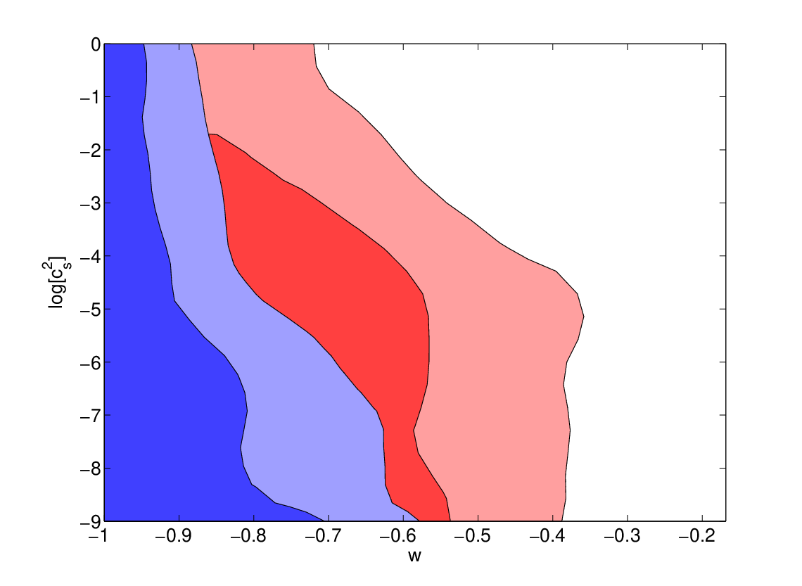


In Figure 4 we plot the and confidence levels expected from Planck and EPIC with and without considering the lensing signal. As we can see, when lensing is considered, is strongly constrained for larger values of . Adding complementary information on such that yields from EPIC at c.l.
On the other hand, the constraints obtained on will probe modified gravity scenarios. In particular, in the case of models, an upper limit of from Planck ( from EPIC) will bound the Compton wavelength to (Planck) and (EPIC). Models that are consistent with solar system test can be significantly ruled out by EPIC. For Chameleons models the bound will be similar with (Planck) and (EPIC).
The accuracy reachable by Planck and EPIC will therefore open the possibility of testing non standard modification to gravity at cosmological length scales ([24]). It is interesting to quantify the impact of a wrong assumption in the lensing potential on the constraints derivable from those experiments and the corresponding ability of recovering the correct solution.


In Figures 5 and 6 we can see the -D likelihood contour plots which show the degeneracies between the lensing parameter and the remaining cosmological parameters. As we can see, a degeneracy appears between and the matter density and the spectral index while a milder degeneracy is also present with the baryon density and the optical depth . A larger value of will make larger values of and and smaller values of and compatible with the CMB data respect to the case with .
Including an uncertainty on will therefore relax the bound on these parameters, especially on and . It is however interesting to quantify the error one could make if not including a marginalization over when analyzing future datasets.
We have therefore changed the fiducial model to for Planck ( for EPIC) and re-analyzed the mock datasets either with the wrong assumption of , either letting to vary,


As we can see from Figures 7 and 8, not accounting for an higher amplitude of the lensing potential could lead to misleading constraints on the baryon density, the cold dark matter density the spectral index and the optical depth. In particular, if we don’t marginalize over we obtain the constraints , , , for Planck and , , and for EPIC to be compared with the fiducial values of , , , . When a marginalization over is included we recover the correct fiducial input parameters.
V Conclusions
In this paper we have investigated the ability of future measurements of CMB temperature and polarization angular spectra to identify a non-standard weak lensing signal. We have found that the amplitude of the weak lensing potential will be measured with a accuracy from Planck ( from EPIC) at confidence level This will let to test the dark energy sound speed parameter for values of the equation of state different from . If, for example, the dark energy of state will be constrained at at c.l. then a value of could be discriminated at more than standard deviations from from an EPIC-like experiment.
Moreover, we have found that both Planck and EPIC could place new constraints on modified gravity models. Translating the bounds on in the case of models on the Compton wavelength we have found that Planck will place a bound of while EPIC will reach . For Chameleons models the bound will be similar with (Planck) and (EPIC). This will present at least a two order of magnitude improvement on the constraint from current CMB data [19]. Finally one should remember that constraints on can be placed by considering higher order correlations and extracting the lensing deflection field from the CMB maps. Several methods have been proposed as the quadratic estimator method (see [39]) and the iterative method by Hirata & Seljak ([40]). Estimating the noise in the case of a quadratic estimator, we have found that a error on could be reached by EPIC of about the same order of the constraint presented here obtained from measurements of the angular power spectra. Since experimental systematics and foregrounds may strongly affect future CMB measurements but affect the angular spectra and the quadratic estimator in a different way the two methods are complementary and will both provide valuable information to the dark energy component.
Acknowledgment
Research work of EC at UC Irvine was supported by NSF CAREER AST-0605427.
AM thanks the University of California Irvine for hospitality.
AS acknowledges financial support from the Berkeley Center for Cosmological Physics. This research
has been supported by ASI contract I/016/07/0 ”COFIS”.
References
- [1] G. Hinshaw et al. [WMAP Collaboration], arXiv:0803.0732 [astro-ph]; E. Komatsu et al., arXiv:0803.0547 [astro-ph].
- [2] J. L. Sievers et al., Astrophys. J. 660 (2007) 976 [arXiv:astro-ph/0509203].
- [3] C. L. Reichardt et al., arXiv:0801.1491 [astro-ph].
- [4] W. C. Jones et al., arXiv:astro-ph/0507494; F. Piacentini et al., arXiv:astro-ph/0507507; arXiv:astro-ph/0507514.
- [5] [Planck Collaboration], arXiv:astro-ph/0604069.
- [6] J. E. Ruhl et al. [The SPT Collaboration], Proc. SPIE Int. Soc. Opt. Eng. 5498, 11 (2004) [arXiv:astro-ph/0411122].
- [7] B. P. Crill et al., arXiv:0807.1548 [astro-ph].
- [8] P. Oxley et al., Proc. SPIE Int. Soc. Opt. Eng. 5543 (2004) 320 [arXiv:astro-ph/0501111].
- [9] J. Bock et al., arXiv:0805.4207 [astro-ph]; J. Bock et al. [EPIC Collaboration and EPIC Collaboration and EPIC Collaboration and ], arXiv:0906.1188 [astro-ph.CO].
- [10] U. Seljak and M. Zaldarriaga, Astrophys. J. 469 (1996) 437 [arXiv:astro-ph/9603033].
- [11] A. Lewis, A. Challinor and A. Lasenby, Astrophys. J. 538 (2000) 473 [arXiv:astro-ph/9911177].
- [12] U. Seljak, N. Sugiyama, M. J. . White and M. Zaldarriaga, Phys. Rev. D 68 (2003) 083507 [arXiv:astro-ph/0306052].
- [13] C. M. Hirata, Phys. Rev. D 78 (2008) 023001 [arXiv:0803.0808 [astro-ph]]; arXiv:0904.2220 [astro-ph.CO].
- [14] G. Efstathiou and J. R. Bond, Mon. Not. Roy. Astron. Soc. 304 (1999) 75 [arXiv:astro-ph/9807103]; R. Bean and A. Melchiorri, Phys. Rev. D 65 (2002) 041302 [arXiv:astro-ph/0110472].
- [15] M. Kowalski et al. [Supernova Cosmology Project Collaboration], Astrophys. J. 686 (2008) 749 [arXiv:0804.4142 [astro-ph]].
- [16] A. Silvestri and M. Trodden, arXiv:0904.0024 [astro-ph.CO].
- [17] R. R. Caldwell and M. Kamionkowski, arXiv:0903.0866 [astro-ph.CO].
- [18] R. K. Sachs and A. M. Wolfe, Astrophys. J. 147 (1967) 73 [Gen. Rel. Grav. 39 (2007) 1929].
- [19] Y. S. Song, H. Peiris and W. Hu, Phys. Rev. D 76 (2007) 063517 [arXiv:0706.2399 [astro-ph]].
- [20] R. Caldwell, A. Cooray and A. Melchiorri, Phys. Rev. D 76, 023507 (2007) [arXiv:astro-ph/0703375]; S. F. Daniel, R. R. Caldwell, A. Cooray and A. Melchiorri, Phys. Rev. D 77 (2008) 103513 [arXiv:0802.1068 [astro-ph]]; S. F. Daniel, R. R. Caldwell, A. Cooray, P. Serra and A. Melchiorri, arXiv:0901.0919 [astro-ph.CO].
- [21] W. Hu, Phys. Rev. D 65 (2002) 023003, eprint astro-ph/0108090.
- [22] M. Kaplinghat, New Astronomy Review, 47, 893, 2003,eprint astro-ph/0307538.
- [23] V. Acquaviva, C. Baccigalupi, 2005, eprint astro-ph/0507644.
- [24] P. Serra, A. Cooray, S. F. Daniel, R. Caldwell and A. Melchiorri, arXiv:0901.0917 [astro-ph.CO].
- [25] M. Kaplinghat et al., Phys. Rev. Lett., 91, 241301, eprint astro-ph/0303344.
- [26] M. Zaldarriaga and U. Seljak, Phys. Rev. D 58 (1998) 023003 [arXiv:astro-ph/9803150]; A. Lewis and A. Challinor, Phys. Rept. 429 (2006) 1 [arXiv:astro-ph/0601594].
- [27] R. Bean and O. Dore, Phys. Rev. D 69 (2004) 083503 [arXiv:astro-ph/0307100].
- [28] A. Lewis and S. Bridle, Phys. Rev. D 66, 103511 (2002) (Available from http://cosmologist.info.)
- [29] [Planck Collaboration], arXiv:astro-ph/0604069.
- [30] D. Baumann et al., arXiv:astro-ph/0811.3919.
- [31] C. P. Ma and E. Bertschinger, Astrophys. J. 455, 7 (1995).
- [32] A. Lewis, Phys. Rev. D 71 (2005) 083008 [arXiv:astro-ph/0502469].
- [33] A. Lewis and A. Challinor, Phys. Rept. 429, 1 (2006).
- [34] G. B. Zhao, L. Pogosian, A. Silvestri and J. Zylberberg, arXiv:0905.1326 [astro-ph.CO].
- [35] W. Hu and I. Sawicki, Phys. Rev. D 76, 064004 (2007) [arXiv:0705.1158 [astro-ph]].
- [36] E. Calabrese, A. Slosar, A. Melchiorri, G. F. Smoot and O. Zahn, Phys. Rev. D 77, 123531 (2008) [arXiv:0803.2309 [astro-ph]].
- [37] K. M. Smith, W. Hu and M. Kaplinghat, Phys. Rev. D 74 (2006) 123002 [arXiv:astro-ph/0607315]; C. Li, T. L. Smith and A. Cooray, Phys. Rev. D 75 (2007) 083501 [arXiv:astro-ph/0607494].
- [38] K. M. Smith, W. Hu and M. Kaplinghat, Phys. Rev. D 70 (2004) 043002 [arXiv:astro-ph/0402442].
- [39] T. Okamoto and W. Hu, Phys. Rev. D 67 (2003) 083002 [arXiv:astro-ph/0301031]; T. Okamoto and W. Hu, Phys. Rev. D 66 (2002) 063008 [arXiv:astro-ph/0206155]; A. Cooray and M. Kesden, New Astron. 8 (2003) 231 [arXiv:astro-ph/0204068]; M. H. Kesden, A. Cooray and M. Kamionkowski, Phys. Rev. D 67 (2003) 123507 [arXiv:astro-ph/0302536].
- [40] C. M. Hirata and U. Seljak, Phys. Rev. D 68 (2003) 083002 [arXiv:astro-ph/0306354].