Pointlike probes of superstring-theoretic superfluids

Liquid Helium, at temperatures below $\sim 2.17{}^{\circ}K$, is the paradigmatic example of a superfluid: a liquid with a broken global symmetry. Since its Helium atom constituents are strongly interacting it is difficult to obtain good theoretical control over the properties of the superfluid beyond the hydrodynamic approximation. This is exactly what the gauge-string duality provides: recent works [1, 2, 3, 4, 5, 6] offer theoretically tractable examples of a strongly coupled superfluid, holographically dual to superconducting black holes in five-dimensional anti-de Sitter space (AdS₅) via the gauge-string duality [7, 8, 9].

In this work we will use a holographic model of a superfluid to study its response to a heavy, pointlike probe. Such an arrangement is similar to an experimental setup where a heavy ion is dragged through superfluid helium [10]. Due to the low viscosity of the superfluid the ion moves without friction until it reaches the critical velocity for quasi-particle creation upon which it slows down. In superfluid helium, the quasi-particle excitations are rotons or vortices, depending on the details of the experimental setup. We will show that in the holographic superfluids we study, there is also a critical velocity which can be determined from the bulk geometry but now the excitations associated with the onset of drag can be thought of as massless. We also study the stochastic force acting on the moving probe and extract from it the transverse and longitudinal mean momentum transfer.¹¹ 1 The formulas for the mean momentum transfer have been obtained independently in [11] in a different context, and a significant simplification of the expression for $\kappa_{L}$ was carried out using techniques borrowed from that work.

Holographic superfluids are different from liquid helium, being based on strongly coupled gauge theories. Moreover, the infrared dynamics of the superfluids we study is characterized by emergent conformal symmetry. The critical velocity that we compute from the low-temperature thermodynamics is the one that the emergent conformal group leaves invariant. It defines an index of refraction of the holographic superfluid. Thus we encounter a surprising confluence of ideas, weaving together superfluidity, emergent symmetry, black hole physics, string dynamics, and refractive signal propagation.

The gauge-string duality allows one to map a theory of gravity in an asymptotically five dimensional AdS space to a strongly coupled, large $N$, $SU(N)$ conformal field theory. Our starting point is the five dimensional bulk action $S={1\over 2\kappa_{5}^{2}}\int d^{5}x\sqrt{-g}\,{\cal L}$ with

From here on, we will set $\kappa_{5}^{2}=1/2$. In [5] it was shown that (1) can be constructed from a truncation of IIB supergravity on a Sasaki-Einstein manifold. (For a related example in M-theory, see [12, 13].) In this truncation, one finds that $\Sigma(\eta)=\sinh^{2}\eta$, $V(\eta)=-{3\over L^{2}}\cosh^{2}{\eta\over 2}(5-\cosh\eta)$, $q=\sqrt{3}/L$ and the real scalars $\eta$ and $\theta$ describe a complex scalar whose target space is the Poincaré disk. This complex scalar is charged under the $U(1)$ gauge field $A_{\mu}$ (where $F=dA$), so non-zero $\eta$ breaks the gauge symmetry. If a solution to the classical equations of motion of (1) is found, then it can be lifted to a solution of type IIB supergravity. As explained in [1, 2] the breaking of the $U(1)$ gauge-symmetry in the bulk corresponds to a formation of a condensate in the boundary theory.

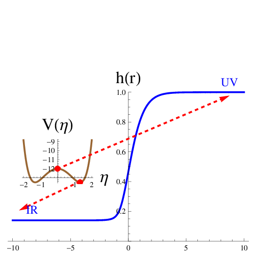
We are interested in the bulk solution which corresponds to a zero temperature configuration where the charged scalar has no non-condensed component. In [14] it was suggested that the zero-temperature limit of black hole solutions of theories similar to (1) would be a domain wall with anti-de Sitter space on both sides: If we parameterize the line element, gauge field, and scalar field as $ds_{M}^{2}=e^{2A(r)}\left(-h(r)dt^{2}+d\vec{x}^{2}\right)+dr^{2}/h(r)$, $A_{\mu}dx^{\mu}=\Phi(r)dt$, $\eta=\eta(r)$, $\theta=0$ then the blackening function $h$ has positive slope everywhere, is approximately $1$ in the ultraviolet (UV) at large positive $r$ and asymptotes to a constant, which we denote $v_{\rm IR}^{2}$, in the infrared (IR) where $r$ is very negative. The warp factor $A(r)$ also has positive slope everywhere and interpolates between two different linear functions of $r$, namely $r/L_{\rm IR}$ in the IR and $r/L$ in the UV. Similarly, the scalar $\eta(r)$ rolls down from a local maximum of the potential $V$ in the ultraviolet to a local minimum in the infrared. Note that $L_{\rm IR}$ and $\eta_{\rm IR}$ are related through $V(\eta_{\rm IR})=-12/L_{\rm IR}^{2}$. We will interpret this domain wall solution, in the dual gauge theory, as the ground state for a finite density of $U(1)$ charge, in which all the charge is carried by a superfluid condensate.

In the case of the IIB Lagrangian discussed above, $\eta_{\rm IR}=\cosh^{-1}2$ and $\eta_{\rm UV}=0$. An explicit domain wall solution for this theory was constructed in [6], where it was found that $v_{\rm IR}\approx 0.373$. This domain wall is a typical example of a zero temperature configuration with conformal invariance in the infrared as well as the ultraviolet. The result of [6] has been reproduced in figure 1.

With the bulk description of a zero temperature superfluid in hand, we examine a heavy pointlike particle moving through the superfluid at constant velocity. On the gravity side this is described by a trailing string, similar to the treatments of [15, 16]. One end of the string is located at the asymptotically AdS₅ boundary and specifies the location of the probe particle in the boundary theory. The other end of the string trails off into the deep IR. The momentum flowing down the string is equal in magnitude to the drag force acting on the boundary theory particle. Thus, to find the drag force one needs to look for an appropriate string configuration and compute the momentum flowing down the string.

We will work with a string action of the form

Here $g_{\mu\nu}$ is the five-dimensional Einstein frame metric and $(\tau,\sigma)$ are worldsheet coordinates. In the particular case of the IIB action considered in [5] one finds that $Q=\cosh{\eta\over 2}$. The procedure of extracting the drag force from the action is straightforward and here we merely quote the result:

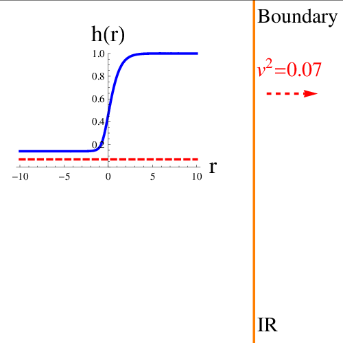
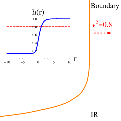
where $A_{*}=A(r_{*})$, $Q_{*}=Q(\eta(r_{*}))$, and so forth, and $r_{*}$ is determined implicitly by the equation $h(r_{*})=v^{2}$. The result (3) (which was basically already understood in [17]) provides some interesting intuition about what warped geometry means: the string frame warp factor on the spatial dimensions $x^{1}$, $x^{2}$, and $x^{3}$ is $e^{2A}Q$, and, up to velocity-independent constants, this string frame warp factor evaluated at $r=r_{*}$ (when $r_{*}$ exists) is the coefficient of kinetic friction for a heavy pointlike probe. The surprising feature of (3) is the appearance of the step function $\Theta$ which vanishes when its argument is negative: Once the velocity of the probe is smaller than $v_{\rm IR}$ then $h_{*}=v^{2}$ has no solution, and the drag force vanishes. This is depicted in figure 2.

By Taylor expanding the drag force, the asymptotic behaviors of $F_{\rm drag}$ as $v$ approaches $1$ from below or $v_{\rm IR}$ from above can be written in terms of the infrared or ultraviolet parameters of the theory,

where $\langle T_{00}\rangle$ is the energy density of the zero temperature configuration in the boundary theory, $\Delta_{\Phi}$ is the dimension of the $U(1)$ current in the infrared defined so that a conserved current has dimension 3, and $b_{h}$ is an extra parameter which characterizes the deviation of $h$ from a constant value in the IR. For the type IIB theory of [5], $\Delta_{\Phi}=5$. The details of the derivation of (3) and (4) can be found in appendix A.

The onset of the drag force in the holographic setup we’ve just described seems to be associated to a phenomenon analogous to roton emission and to Cherenkov radiation—the latter providing a slightly closer analogy, as we now explain. Low-energy photons in a refractive medium comprise a free conformal field theory with a reduced speed of propagation relative to the speed of light in vacuum. When an electrically charged particle travels through the medium faster than the speed of light, nearly free photons are emitted in a process called Cherenkov radiation. What probably happens in our setup is that an operator which couples to the pointlike probe mediates strongly interacting “radiation” into the medium, and this radiation propagates at a velocity $v_{\rm IR}$.²² 2 We thank D. Son for discussions on this point. Although this line of thought is plausible, it surprises us that the scaling $F_{\rm drag}\sim(v-v_{\rm IR})^{a}$ for $v$ slightly larger than $v_{\rm IR}$ is characterized by an exponent $a=(\Delta_{\Phi}-4)^{-1}$: The spectral measure of the two-point function of the operator that the probe couples to is the analog of phase space for photons emitted through the Cherenkov process. Naive phase space measure arguments applied to the case of weakly coupled quasi-particle emission suggest instead a scaling exponent $a\sim\Delta$, where $\Delta$ is the dimension of the operator responsible for the quasi-particle emission. An extension of these phase space arguments to strongly coupled theories, à la [18], still gives an $a\sim\Delta$ scaling where $\Delta$ would now be the dimension of the “quasi-unparticles.” Perhaps a better understanding of how ultraviolet cutoffs affect the strongly coupled radiation rate would resolve the quandary of the scaling of $a$; or perhaps there is an operator mediating the radiation whose anomalous dimension in the infrared is inversely proportional to $\Delta_{\Phi}$. This issue certainly warrants further attention.

In [19] it was shown that a relativistic gas of particles in the grand canonical ensemble with dispersion relation $\omega=kc_{q}$ leads to a relation of the form $c_{q}^{2}=sT/(sT+\mu\rho)$ where $s$ is the entropy density, $T$ is the temperature, $\mu$ is the chemical potential, and $\rho$ is the charge density of the quasi-particles. We now show, using arguments entirely on the gravity side, that a similar relation holds in the low-temperature limit for solutions of (1):

where $\rho_{n}$ is the density of $U(1)$ charge in the normal state, defined as in [20] by the thermodynamic relation $dP=s\,dT+\rho_{n}\,d\mu-{\rho_{s}\over 2\mu}d\xi^{2}$, where $\xi_{m}=\partial_{m}\varphi$ and $\varphi$ is the Goldstone boson of the broken $U(1)$ symmetry. In our derivation, we will not require the assumption that there are low-energy quasi-particles that propagate with speed $v_{\rm IR}$.

To prove (5) we use the formalism developed in [20]. So far we considered the zero temperature solution of the theory. If the temperature is finite then the solution will be a black hole, by which we mean that the infrared limit of the theory is characterized in the bulk by a black hole horizon at $r=r_{0}$ where $h(r_{0})=0$. The transition from a black hole solution to a domain wall solution occurs by the blackening function $h$ developing a “double shelf” structure. That is, the horizon is pushed to the deep IR, before which $h$ is characterized by a region where it is approximately constant at a value approaching $v_{\rm IR}^{2}$. The double shelf structure was first discussed in [21].

In these positive but low temperature solutions, we consider vector perturbations of the stationary metric of the form $A_{x^{1}}=a(r)$ and $g_{tx^{1}}=e^{2A(r)}g(r)$, and solve the linearized equations of motion for $g$ and $a$. The explicit form for the equation of motion for $g$ can be written as a total derivative by making use of the equations of motion for the background solution. After integrating it once it takes the form $e^{4A}g^{\prime}+e^{2A}a\Phi^{\prime}=Q_{2}$ where $Q_{2}$ is an integration constant. By expanding the fields $a$ and $g$ near the boundary and using the relativistic two-fluid model for superfluids, introduced in [22] and elaborated upon in [4, 23, 20], one can show that $Q_{2}=sTu_{x^{1}}+(u_{x^{1}}-v_{x^{1}})\mu\rho_{n}$. Where $\vec{u}$ and $\vec{v}$ are the velocity of the normal component and the superfluid velocity respectively. This leads to $Q_{2}=sTu_{x^{1}}+(u_{x^{1}}-v_{x^{1}})\mu\rho_{n}$. Making use of Lorentz invariance, a similar analysis can be carried out for the equation of motion for $a$. One finds $he^{2A}(a\phi^{\prime}-a^{\prime}\phi)=hQ_{2}-gQ_{1}+Q_{3}$ with $Q_{3}=(v_{x}-u_{x})\mu\rho_{\rm n}$. To obtain (5) we can evaluate the equation of motion for $a$ on the “infrared shelf” described earlier, and then take the zero temperature limit. The finer details of this analysis are left to appendix B.

Considering (5) together with the computation of [19] and the expression for the drag force for $v$ near $v_{\rm IR}$, it is tempting to speculate that the low temperature thermal excitations are massless particles. However, one should keep in mind that our system is strongly coupled, so it’s more likely that the critical velocity is associated with a strongly coupled “soup” of excitations whose collective behavior is in some ways similar to that of massless particles, but cannot be fully described in terms of quasi-particles.

Having determined the drag force acting on the probe particle and related the threshold velocity $v_{\rm IR}$ at which it becomes non-zero to thermodynamic quantities, we proceed to compute the stochastic forces on the probe. In a Langevin formalism with white noise, one expresses the total force acting on the probe as $d\vec{p}/dt\equiv\vec{F}_{\rm tot}=\vec{F}_{\rm drag}+\vec{F}_{L}(t)+\vec{F}_{T}(t)$, where $\vec{F}_{L}(t)$ is the stochastic force in the same direction as the motion of the probe particle while $\vec{F}_{T}(t)$ is orthogonal to it. The expectation values of $\vec{F}_{L}$ and $\vec{F}_{T}$ vanish, while $\langle F_{L}^{i}(t_{1})F_{L}^{j}(t_{2})\rangle=\kappa_{L}\hat{p}^{i}\hat{p}^{j}\delta(t_{1}-t_{2})$ and $\langle F_{T}^{i}(t_{1})F_{T}^{j}(t_{2})\rangle=\kappa_{T}(\delta^{ij}-\hat{p}^{i}\hat{p}^{j})\delta(t_{1}-t_{2})$, where $\hat{p}^{i}$ is the unit vector in the direction of the momentum $\vec{p}$.

In [24, 25, 26] it was shown explicitly that the stochastic force $\vec{F}_{L}+\vec{F}_{T}$ owes to the existence of a horizon on the string worldsheet: the endpoint of the string on the boundary is causally accessible to only that part of the string worldsheet with $r>r_{*}$, where $r_{*}$ is determined as before from $h_{*}=v^{2}$. (If $v<v_{\rm IR}$, then there is no worldsheet horizon. We will focus on the case $v_{\rm IR}<v<1$ from now on.) The metric on the string worldsheet above the horizon can be written in diagonal form $ds_{WS}^{2}=\gamma_{ab}d\sigma^{a}d\sigma^{b}=-e^{2A}(h-v^{2})d\tau^{2}+\left({1\over h}+{e^{2A}h\xi^{\prime 2}\over h-v^{2}}\right)dr^{2}$, where the worldsheet coordinates $(\tau,r)$ are specified by the indices $a,b$. Note that $\tau=t$ only on the boundary. The worldsheet Hawking temperature is given by

Following arguments similar to the ones leading to (4), one finds

provided $Q$ approaches a constant in the UV and IR. When $\Delta_{\phi}=5$ then $T_{WS}$ is linear in $v-v_{\rm IR}$ for $v$ close to $v_{\rm IR}$.

To study the stochastic forces further, one should consider perturbations of the string around the trailing string solution which lead to the drag force result (3). Computations of this sort where carried out in [25, 26, 27, 28] and can be extended to general holographic backgrounds of the form we’ve discussed. The technique for carrying out this extension is to use the method of matched asymptotic expansions for approximate expressions for the fluctuations at small frequency and in the deep infrared. The result is

The details of this computation are left to appendix C. We note that the form of $\kappa_{T}$ is interestingly similar to the Einstein relation $\kappa^{\rm Einstein}_{L}=-{2F_{\rm drag}T/v}$, which can be derived by demanding that stochastic evolution based on the total drag force $\vec{F}_{\rm tot}$ equilibrates to a thermal distribution of temperature $T$, see for example [29]. But the differences between $\kappa_{T}$ and $\kappa^{\rm Einstein}_{L}$ are significant: besides constraining $\kappa_{T}$ rather than $\kappa_{L}$, the involvement of $T_{WS}$ in the expression for $\kappa_{T}$ makes it hard for us to see what the late-time equilibrium distribution of momenta would be when the probe mass is made finite.

We thank C. Herzog, A. Nellore and D. Son for useful discussions. This work was supported in part by the Department of Energy under Grant No. DE-FG02-91ER40671 and by the NSF under award number PHY-0652782.

References

- [1] S. S. Gubser, “Breaking an Abelian gauge symmetry near a black hole horizon,” Phys. Rev. D78 (2008) 065034, 0801.2977.
- [2] S. A. Hartnoll, C. P. Herzog, and G. T. Horowitz, “Building a Holographic Superconductor,” Phys. Rev. Lett. 101 (2008) 031601, 0803.3295.
- [3] P. Basu, A. Mukherjee, and H.-H. Shieh, “Supercurrent: Vector Hair for an AdS Black Hole,” 0809.4494.
- [4] C. P. Herzog, P. K. Kovtun, and D. T. Son, “Holographic model of superfluidity,” 0809.4870.
- [5] S. S. Gubser, C. P. Herzog, S. S. Pufu, and T. Tesileanu, “Superconductors from Superstrings,” 0907.3510.
- [6] S. S. Gubser, S. S. Pufu, and F. D. Rocha, “Quantum critical superconductors in string theory and M- theory,” 0908.0011.
- [7] J. M. Maldacena, “The large N limit of superconformal field theories and supergravity,” Adv. Theor. Math. Phys. 2 (1998) 231–252, hep-th/9711200.
- [8] S. S. Gubser, I. R. Klebanov, and A. M. Polyakov, “Gauge theory correlators from non-critical string theory,” Phys. Lett. B428 (1998) 105–114, hep-th/9802109.
- [9] E. Witten, “Anti-de Sitter space and holography,” Adv. Theor. Math. Phys. 2 (1998) 253–291, hep-th/9802150.
- [10] D. R. Allum, P. V. E. McClintock, A. Phillips, and R. M. Bowley, “The Breakdown of Superfluidity in Liquid 4He: An Experimental Test of Landau’s Theory,” Phil. Trans. R. Soc. 284 (1977) 179–224.
- [11] C. Hoyos-Badajoz, “Drag and jet quenching of heavy quarks in a strongly coupled N=2* plasma,” 0907.5036.
- [12] J. P. Gauntlett, S. Kim, O. Varela, and D. Waldram, “Consistent supersymmetric Kaluza–Klein truncations with massive modes,” JHEP 04 (2009) 102, 0901.0676.
- [13] J. P. Gauntlett, J. Sonner, and T. Wiseman, “Holographic superconductivity in M-Theory,” 0907.3796.
- [14] S. S. Gubser and F. D. Rocha, “The gravity dual to a quantum critical point with spontaneous symmetry breaking,” Phys. Rev. Lett. 102 (2009) 061601, 0807.1737.
- [15] C. P. Herzog, A. Karch, P. Kovtun, C. Kozcaz, and L. G. Yaffe, “Energy loss of a heavy quark moving through N = 4 supersymmetric Yang-Mills plasma,” JHEP 07 (2006) 013, hep-th/0605158.
- [16] S. S. Gubser, “Drag force in AdS/CFT,” Phys. Rev. D74 (2006) 126005, hep-th/0605182.
- [17] C. P. Herzog, “Energy loss of heavy quarks from asymptotically AdS geometries,” JHEP 09 (2006) 032, hep-th/0605191.
- [18] H. Georgi, “Unparticle Physics,” Phys. Rev. Lett. 98 (2007) 221601, hep-ph/0703260.
- [19] B. Carter and D. Langlois, “The Equation of state for cool relativistic two constituent superfluid dynamics,” Phys. Rev. D51 (1995) 5855–5864, hep-th/9507058.
- [20] C. P. Herzog and A. Yarom, “Sound modes in holographic superfluids,” 0906.4810.
- [21] S. S. Gubser and A. Nellore, “Low-temperature behavior of the Abelian Higgs model in anti-de Sitter space,” JHEP 04 (2009) 008, 0810.4554.
- [22] D. T. Son, “Hydrodynamics of relativisic systems with broken continuous symmetries,” Int. J. Mod. Phys. A16S1C (2001) 1284–1286, hep-ph/0011246.
- [23] A. Yarom, “Fourth sound of holographic superfluids,” 0903.1353.
- [24] J. Casalderrey-Solana and D. Teaney, “Heavy quark diffusion in strongly coupled N = 4 Yang Mills,” hep-ph/0605199.
- [25] S. S. Gubser, “Momentum fluctuations of heavy quarks in the gauge-string duality,” Nucl. Phys. B790 (2008) 175–199, hep-th/0612143.
- [26] J. Casalderrey-Solana and D. Teaney, “Transverse Momentum Broadening of a Fast Quark in a N=4 Yang Mills Plasma,” hep-th/0701123.
- [27] G. C. Giecold, E. Iancu, and A. H. Mueller, “Stochastic trailing string and Langevin dynamics from AdS/CFT,” 0903.1840.
- [28] D. T. Son and D. Teaney, “Thermal Noise and Stochastic Strings in AdS/CFT,” JHEP 07 (2009) 021, 0901.2338.
- [29] G. D. Moore and D. Teaney, “How much do heavy quarks thermalize in a heavy ion collision?,” Phys. Rev. C71 (2005) 064904, hep-ph/0412346.
- [30] U. Gursoy, E. Kiritsis, G. Michalogiorgakis, and F. Nitti, “Thermal Transport and Drag Force in Improved Holographic QCD,” 0906.1890.
- [31] S. S. Gubser, “Time warps,” 0812.5107.