Segmentation for radar images based on active contour

Weather radar data quality control is extremely important for meteorological and hydrological applications. For weather radars, scatterers in the atmosphere are not only meteorological particles like cloud, rain drops, snowflakes, and hails, but also non-meteorological particles such as chaff, insects, and birds. For radar meteorologists it is a major issue and challenge to design numerical scheme which can automatically and subjectively distinguish meteorological echoes from non-meteorological echoes. Non-meteorological echoes can contaminate radar reflectivity and Doppler velocity measurements, and subsequently cause errors and uncertainty on radar data applications in quantitative precipitation estimation, as well as in assimilation in numerical model for weather prediction. Automatic detection of tornado or mesocyclone vortex among meteorological echoes is certainly another big challenge and has great potential in improving severe weather forecast and saving human life.

For different echoes, their graphic properties such as pattern, intensity and texture, are different. See, for example, fig. 1. Such differences enable us to design new active contour model to automatically extract the most distinguishing graphic properties from echoes, and to segment them easily from other noises. Our methods shall also be very useful in automatic detection of tornadic supercell, as well as in storm classifications and tracking in the future study.

Active contour is the procedure that we deform a given curve so that a given functional of the curve will achieve its local minimal value. This method is wildly used recently in computer vision in seeking the edges or contours of given images. See, for example, Mumford and Shah [4], Kass, Witkin and Terzopoulos [3], Caselles, Kimmel and Sapiro [1], and Chan and Vese [2].

Let $u_{0}(x,y):\Omega\to R$ be the gray level function of a given image. If $u_{0}$ is smooth, then the edge of the image are those points $(x,y)$ where $|\nabla u_{0}|$ is relatively large.

The geometric contour and snake models aim to detect edge automatically based on the size of $|\nabla u_{0}|$. Let $C(s):[0,L]\to\mathbb{R}^{2}$ be a closed curve, where $s$ is its arc length parameter. One can introduce an edge-detector function $g:\Omega\to R_{+}$ so that $g(z)\to 0$ as $z\to\infty$. A typical example of such function is given by

$$g(z)=\frac{1}{1+z^{2}}.$$

We define the energy functional of $C$ by

(2.1)

$$I_{1}(C):=\int_{0}^{L}g(\nabla u_{0}(C(s)))ds,$$

then to find the edge of image $u_{0}$ can be reduced to seek the local minimal for $I_{1}$ (the geometric active contour model [1]):

(2.2)

$$I_{1}(edge)=inf_{C}I_{1}(C).$$

The snake model [3] is to introduce, for a parameterized curve $C(p):[0,1]\to\mathbb{R}^{2}$, the following energy functional :

(2.3)

$$I_{2}(C)=\alpha\int_{0}^{1}|C^{\prime}(p)|^{2}dp+\beta\int_{0}^{1}|C^{\prime\prime}(p)|dp-\lambda\int_{0}^{1}|\nabla u_{0}(C(p))|^{2}dp,$$

where $\alpha,\beta,\lambda$ are all positive parameters. The first two terms represent the internal energy of the image, which usually are used to smooth the curve; The third term represents the external energy, serving as the indicator for edge. The edge of the image then can be found by minimizing $I_{2}$:

(2.4)

$$I_{2}(edge)=\inf_{C}I_{2}(C).$$

To automatically detect the edge via an iteration scheme, one introduces a family of curves $C(p,t):[0,1]\times[0,\infty)\to\mathbb{R}^{2}$ and the deformation path. For example, for active contour model (2.2) the curve evolution (gradient flow equation) is given by

(2.5)

$$C_{t}=(kg-\nabla g\cdot\mathbf{N})\mathbf{N},$$

where $k$ is the curvature function and $\mathbf{N}$ is the inner unit normal vector of curve $C(p,t).$

Numerically, such iteration can be realized via the powerful level set method of Osher and Sethian [5]. Embed $C(p,t)$ as a nodal line of a smooth function $\Phi(x,y,t)$: $C=\{(x,y,t)\ :\ \Phi(x,y,t)=0\}$. From $\partial_{t}\Phi(C,t)=0$, we are led to evolve $\Phi$ by

(2.6)

$$\left\{\,\vbox{\halign{$\displaystyle{#}$\hfil&\quad$\displaystyle{{}#}$\hfil\cr\mathstrut\crcr\kern-15.0pt\cr&\frac{\partial\Phi}{\partial t}=g(|\nabla u_{0}|)div(\frac{\nabla\Phi}{|\nabla\Phi|})|\nabla\Phi|+<\nabla g,\nabla\Phi>\\&\Phi(x,y,0)=\Phi_{0}(x,y),\crcr\mathstrut\crcr\kern-15.0pt\cr}}\,\right.$$

where $\Phi_{0}(x,y)$ is the initial level set function. In practice, one can choose $\Phi_{0}(x,y)$ to be a signed distance function to a given initial curve $C(p,0)$. Fig. 2 (b), fig. 3 (b), and fig. 4 (b) show the result for image processing based on such scheme.

If the given image $u_{0}(x,y)$ is not smooth, the edge of the image is not well defined based on the derivative of the gray level function. The human being’s perspective for the edge of a non smooth image basically is to identify the boundary of different groups. To identify such boundary, one can use Chan-Vese energy [2]:

	$\displaystyle I_{3}(C,c_{1},c_{2}):$	$\displaystyle=\int_{inside(C)}|u_{0}-c_{1}|^{2}dxdy+\int_{outside(C)}|u_{0}-c_{2}|^{2}dxdy$
(2.7)			$\displaystyle+\mu\cdot\mbox{(}length(C))+\nu\cdot\mbox{(}Area(inside(C))),$

where $c_{1}$, $c_{2}$ are constants to be adjusted in iteration, $\mu$ and $\nu$ are fixed parameters. The last two terms are smoothing terms. The edge is again sought by minimizing $I_{3}(C,c_{1},c_{2})$:

(2.8)

$$I_{3}(edge,c_{1,*},c_{2,*})=\inf_{C,c_{1},c_{2}}I_{3}(C,c_{1},c_{2}).$$

Again, numerically level set method can be used for such deformation. Introduce the Heaviside function and its derivative

$$H(z)=\left\{\,\vbox{\halign{$\displaystyle{#}$\hfil&\quad$\displaystyle{{}#}$\hfil\cr\mathstrut\crcr\kern-15.0pt\cr&1,\ \ \ \mbox{if}\ \ z\geq 0\\&0,\ \ \ \mbox{if}\ \ z\geq 0,\crcr\mathstrut\crcr\kern-15.0pt\cr}}\,\right.\ \ \ \ \ \ \delta(z)=\frac{d}{dz}H(z).$$

Embedding $C(p,t)$ as a nodal line of a smooth function $\Phi(x,y,t)$: $C=\{(x,y,t)\ :\ \Phi(x,y,t)=0\}$, we can re-write the energy functional $I_{3}(C,c_{1},c_{2})$ as

	$\displaystyle J_{3}(\Phi,c_{1},c_{2}):$	$\displaystyle=\int_{\Omega}|u_{0}-c_{1}|^{2}H(\Phi(x,y))dxdy+\int_{\Omega}|u_{0}-c_{2}|^{2}(1-H(\Phi(x,y)))dxdy$
(2.9)			$\displaystyle+\mu\int_{\Omega}\delta(\Phi(x,y))|\nabla\Phi(x,y)|dxdy+\nu\int_{\Omega}H(\Phi(x,y))dxdy.$

For fixed $\Phi$, minimizing $J_{3}(\Phi,c_{1},c_{2})$ with respect to $c_{i}$ yields

$$\left\{\,\vbox{\halign{$\displaystyle{#}$\hfil&\quad$\displaystyle{{}#}$\hfil\cr\mathstrut\crcr\kern-15.0pt\cr&c_{1}(\Phi)=\mbox{average}(u_{0})\ \mbox{in}\ \{\Phi<0\}\\&c_{2}(\Phi)=\mbox{average}(u_{0})\ \mbox{in}\ \{\Phi\geq 0\}.\crcr\mathstrut\crcr\kern-15.0pt\cr}}\,\right.$$

Once $c_{1}$ and $c_{2}$ are fixed, we minimize $J_{3}$ via deforming $\Phi$ along the gradient direction:

(2.10)

$$\left\{\,\vbox{\halign{$\displaystyle{#}$\hfil&\quad$\displaystyle{{}#}$\hfil\cr\mathstrut\crcr\kern-15.0pt\cr&\frac{\partial\Phi}{\partial t}=\delta(\Phi)\big\{\mu\cdot div(\frac{\nabla\Phi}{|\nabla\Phi|})-\nu-(u_{0}-c_{1}(\Phi))^{2}+(u_{0}-c_{2}(\Phi))^{2}\big\}\ \ \ \mbox{in}\ \ \ (0,\infty)\times\Omega,\\&\Phi(x,y,0)=\Phi_{0}(x,y)\ \ \ \ \ \mbox{in}\ \ \ \Omega,\\&\frac{\delta(\Phi)}{|\nabla\Phi|}\frac{\partial\Phi}{\partial n}=0\ \ \ \ \ \ \ \mbox{on }\ \ \ \partial\Omega\crcr\mathstrut\crcr\kern-15.0pt\cr}}\,\right.$$

where $\Phi_{0}(x,y)$ is a signed distance function to a given initial curve $C(p,0)$. Fig. 2 (c), fig. 3 (c), and fig. 4 (c) show the result for image processing based on such scheme.

As being pointed out in [2], The Chan-Vese model is originated in the Mumform-Shah model [4]:

	$\displaystyle F^{MS}(u,C)=\mu\cdot length(C)$	$\displaystyle+\lambda\int_{\Omega}|u_{0}(x,y)-u(x,y)|^{2}dxdy$
		$\displaystyle+\int_{\Omega\setminus C}|\nabla u(x,y)|^{2}dxdy,$

where $u_{0}:\overline{\Omega}\to\mathbb{R}$ is the given image, $K\subset\Omega$ is the curve that we will deform. The sharp boundary of $u_{0}$, where $|\nabla u_{0}|$ is large or discontinuous can be detected via minimizing $F^{MS}(u,C)$. Roughly speaking, if we replace $u$ by a constant function in the above, we can see the prototype model similar to that of Chan-Vese. These models are all viewed as minimal partition problems.

We observe that radar noises usually have relatively low intensity to severe storms, and radar signals for storm are usually uniform in certain region. To segment the severe storm from usual radar noises, we introduce the following modified Chan-Vese functional:

	$\displaystyle I_{4}(C,c):$	$\displaystyle=\int_{inside(C)}|u_{0}-\alpha\cdot M|^{2}dxdy+\int_{outside(C)}|u_{0}-c|^{2}dxdy$
(3.1)			$\displaystyle+\mu\cdot\mbox{(}length(C))+\nu\cdot\mbox{(}Area(inside(C))),$

where $M=\max_{x\in\Omega}u_{0}(x)$, $c$ is a constant to be adjusted in iteration, $\alpha$, $\mu$ and $\nu$ are fixed parameters. In practice, parameter $\alpha$ can be determined by comparing the maximal intensity near radar and the maximal intensity of storm.

Embedding $C(p,t)$ as a nodal line of a smooth function $\Phi(x,y,t)$: $C=\{(x,y,t)\ :\ \Phi(x,y,t)=0\}$, we can re-write the energy functional $I_{4}(C,c)$ as

	$\displaystyle J_{4}(\Phi,c):$	$\displaystyle=\int_{\Omega}|u_{0}-\alpha\cdot M|^{2}H(\Phi(x,y))dxdy+\int_{\Omega}|u_{0}-c|^{2}(1-H(\Phi(x,y)))dxdy$
(3.2)			$\displaystyle+\mu\int_{\Omega}\delta(\Phi(x,y))|\nabla\Phi(x,y)|dxdy+\nu\int_{\Omega}H(\Phi(x,y))dxdy.$

For fixed $\Phi$, minimizing $J_{4}(\Phi,c)$ with respect to $c$ yields

$$c(\Phi)=\mbox{average}(u_{0})\ \mbox{in}\ \{\Phi\geq 0\}.$$

To derive the first variation of the functional, we consider slightly regularized version of functions $H_{\epsilon}$ and $H^{\prime}_{\epsilon}=\delta_{\epsilon}$ such that $H_{\epsilon}\in C^{(}\overline{\Omega})$, $H_{\epsilon}\to H$ and $\delta_{\epsilon}\to\delta$, and the modified functional:

	$\displaystyle J_{4,\epsilon}(\Phi,c):$	$\displaystyle=\int_{\Omega}|u_{0}-\alpha\cdot M|^{2}H_{\epsilon}(\Phi(x,y))dxdy+\int_{\Omega}|u_{0}-c(\Phi)|^{2}(1-H_{\epsilon}(\Phi(x,y)))dxdy$
(3.3)			$\displaystyle+\mu\int_{\Omega}\delta_{\epsilon}(\Phi(x,y))|\nabla\Phi(x,y)|dxdy+\nu\int_{\Omega}H_{\epsilon}(\Phi(x,y))dxdy.$

Its first variation is

	$\displaystyle<\delta J_{4,\epsilon},\psi>$	$\displaystyle=\int_{\Omega}(u_{0}-\alpha\cdot M)^{2}\delta_{\epsilon}(\Phi(x,y))\psi dxdy-\int_{\Omega}(u_{0}-c(\Phi))^{2}\delta_{\epsilon}(\Phi(x,y))\psi dxdy$
		$\displaystyle+\mu\int_{\Omega}\delta_{\epsilon}(\Phi(x,y))\frac{\nabla\Phi}{|\nabla\Phi(x,y)|}\nabla\psi dxdy+\nu\int_{\Omega}\delta_{\epsilon}(\Phi(x,y))\psi dxdy.$

Thus we can minimize $J_{4,\epsilon}$ via deforming $\Phi$ along its gradient direction:

(3.4)

$$\left\{\,\vbox{\halign{$\displaystyle{#}$\hfil&\quad$\displaystyle{{}#}$\hfil\cr\mathstrut\crcr\kern-15.0pt\cr&\frac{\partial\Phi}{\partial t}=\delta_{\epsilon}(\Phi)\big\{\mu\cdot div(\frac{\nabla\Phi}{|\nabla\Phi|})-\nu-(u_{0}-\alpha\cdot M)^{2}+(u_{0}-c(\Phi))^{2}\big\}\ \ \ \ \ \mbox{in}\ \ (0,\infty)\times\Omega,\\&\Phi(x,y,0)=\Phi_{0}(x,y)\ \ \ \ \ \ \ \mbox{in}\ \ \ \Omega,\\&\frac{\delta_{\epsilon}(\Phi)}{|\nabla\Phi|}\frac{\partial\Phi}{\partial n}=0\ \ \ \ \ \ \ \mbox{on}\ \ \ \partial\Omega.\crcr\mathstrut\crcr\kern-15.0pt\cr}}\,\right.$$

An image of reflectivity factor field of tornadic supercells, observed by a S-band weather radar near Oklahoma City, Oklahoma, is presented in Fig.1(a). The violent tornadoes generated from the weather system ripped through Oklahoma and Kansas and killed 48 people while demolishing houses and business. It had caused at least $\$500$ M in property damage (http://www.nssl.noaa.gov/headlines/outbreak.shtml).

We first use geodesic active contour model (2.6) for the image. It results in catching all boundaries, including radar noises (fig. 2 (b)). We then apply standard Chan-Vese model (2.10) with $\mu=5$, $\nu=0$ (fig. 2(c)). Still it keeps almost all boundaries from radar noises. We finally apply our model (3.4) with $\alpha=0.7$ in fig. 2 (d). The result shows that almost all radar noises are successfully skipped.

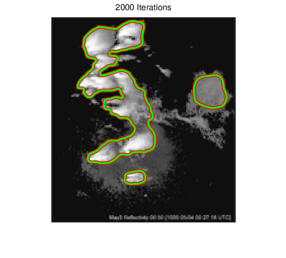
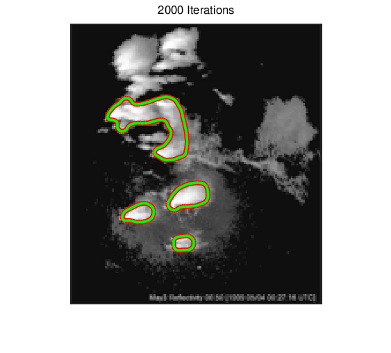
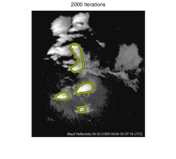
Fig. 3 (a) usually is a challenge radar image for processing. The radar noises are embedded in storm image (in fact, radar is underneath the cloud). Geodesic active contour is very sensitive to the initial curve. It usually contracts curve. Fig. 3 (b) is a failure via geodesic active contour. Fig. 3 (c) is the result using Chan-Vese model (choose $\mu=5$, $\nu=0$); Fig. 3 (d) is based on our model (3.4) (with $\alpha=0.4$). There is no big difference between fig. 3 (c) and fig. 3 (d).

Fig. 4 (a) is another radar image with radar noise separated from storm. Chan-Vese can not remove radar noise completely. Our model with suitable parameter ( $\alpha=.6$) works fine.

Finally, we compare the results using Chan-Vese model and our model with different parameters.

First we consider Chan-Vese model with different parameters:

(4.1)

$$\left\{\,\vbox{\halign{$\displaystyle{#}$\hfil&\quad$\displaystyle{{}#}$\hfil\cr\mathstrut\crcr\kern-15.0pt\cr&\frac{\partial\Phi}{\partial t}=\delta(\Phi)\big\{\mu\cdot div(\frac{\nabla\Phi}{|\nabla\Phi|})-\nu-\lambda(u_{0}-c_{1}(\Phi))^{2}+(u_{0}-c_{2}(\Phi))^{2}\big\}\\&\Phi(x,y,0)=\phi_{0}(x,y),\crcr\mathstrut\crcr\kern-15.0pt\cr}}\,\right.$$

where $\lambda$ is a positive parameter. The results using Chan-Vese model with different $\lambda$ are presented in fig. 5.

Next we compare the results using our model with different $\alpha$ in fig. 6. It can be seen that for $\alpha$ in certain range, our results are relatively stable. Therefore, for different $\alpha$, if we let

$$c_{\alpha}^{out}(\Phi)=\mbox{average}(u_{0})\ \mbox{in}\ \{\Phi<0\},$$

we can develop a program which can automatically determine which $\alpha$ we shall choose based on the changing of $c_{\alpha}^{out}(\Phi)$ as $\alpha$ changes.

We compare various models and their applications to the segmentation of radar images. We propose our new model. Our method is more efficient in outlining more severe storm images, and skipping the usual radar noises.

References

- [1] Caselles, V.; Kimmel, R.; Sapiro, G., Geodesic active contours, Int. Journal of Computer Vision 22 (1997), no. 11, 61-79.
- [2] T. Chan and L. Vese, Active contours without edges, IEEE Transactions on Image Processing, Vol. 2, 2001, 266-277.
- [3] Kass, M.; Witkin, A.; Terzopoulos, D., Snakes: active contour models, Int. Journal of Computer Vision 1 (1987), 321-331.
- [4] D. Mumford; J. Shah, Optimal approximations by piecewise smooth functions and associated variational problems. Comm. Pure Appl. Math. 42 (1989), no. 5, 577–685.
- [5] S. Osher and J. Sethian, Fronts propagating with curvature-dependent speed: algorithms based on Hamilton-Jacobi formulations. J. Comput. Phys. 79 (1988), no. 1, 12–49.