The cranking formula and the spurious behaviour of the mass parameters

The mass (or vibrational) parameters are given by the Inglis formula [1], [3]:

Where $\left|O\right\rangle,\left|M\right\rangle$ are respectively the ground state and the excited states of the nucleus. The quantities $E_{M},E_{O}$ are the associated eigenenergies. In the independent-particle model, whenever the state of the nucleus is assumed to be a Slater determinant (built on single-particle states of the nucleons), the ground state$\left|O\right\rangle$ will be of course the one where all the particles occupy the lowest states. The excited states $\left|M\right\rangle$ will be approached by the one particle-hole configurations. In that case, Eq. (2) becomes (see appendix A ):

$\lambda$ denotes the Fermi level. The above expression can be simplified further if the following simple property is used:
$\left(\epsilon_{k}-\epsilon_{l}\right)\left\langle k\right|\partial$ $/\partial\beta_{j}\left|l\right\rangle=\left\langle k\right|\left[H_{sp},\partial/\partial\beta_{j}\right]\left|l\right\rangle=-\left\langle k\right|\partial H_{sp}/\partial\beta_{j}\left|l\right\rangle$ for $k\neq l$
so that Eq. (3) becomes

where $H_{sp}$ is the single-particle hamiltonian. The single particle states are given by the Schrodinger equation of the independent-particle model.

It must be noted that in Eq. (4) the denominator $\epsilon_{l}-\epsilon_{k}$ vanishes in the case where the Fermi level coincides with two or more degenerate levels. This is the major drawback of the formula. It is possible to overcome this difficulty by taking into account the pairing correlations. This can be achieved through the BCS approximation by the following replacements in Eq. (2):
  i) the ground state $\left|O\right\rangle$ by the BCS state $\left|BCS\right\rangle.$
  ii) the excited states $\left|M\right\rangle$ by the two quasiparticle excitations states $\left|\mu,\nu\right\rangle$ (here we consider only the even-even nuclei). This led Belyaev [7] to two types of non-vanishing matrix elements (see also the demonstration given in the appendix B):

The later is due to the changing of the occupations probabilities with the deformation, i.e. with $u_{\nu}$ and $\upsilon_{\nu}$:
  iii) the energy $E_{O\text{ }}$ by $E_{BCS}$ and $E_{M}$ by the energy of the two quasiparticles, i.e., by $E_{\nu}+E_{\mu}+E_{BCS}$. The quasiparticle energy being $E_{\nu}=\sqrt{\left(\epsilon_{\nu}-\lambda\right)^{2}+\Delta^{2}}$ and the BCS state is defined from the ”true” vacuum $\left|0\right\rangle$ by: $\left|BCS\right\rangle=\Pi_{k}\left(u_{k}+\upsilon_{k}a_{k}^{+}a_{-k}^{+}\right)\left|0\right\rangle$.
The ”Belyaev formulation” for the mass parameters (formula (53) of the appendix B) is then:

Beside this formula, there is an other more convenient formulation due to Bes [8] modified slightly by the authors of Ref. [1]. In the latter, the above two types of matrix elements have been cast under a more explicit form (see again the demonstrations in appendices C and D),

The final formula of the mass parameters takes now the form (cf. formula (55) of the appendix D):

where

The two quantities of the r.h.s of Eq. (11) are in the adopted order, the so-called ”non-diagonal” and the ”diagonal” parts of the mass parameters. The derivatives are contained in the above diagonal term $R_{i}^{\nu}$. When the derivatives $\partial\lambda/\partial\beta_{i}$, $\partial\Delta/\partial\beta_{i}$ cancel the diagonal term reduce simply to the diagonal matrix element $-\left\langle\nu\right|\partial H_{sp}/\partial\beta_{i}\left|\nu\right\rangle$. In order to facilitate the comparison with other papers, we recall that the cranking formula is usually cast under a slightly different form:

where the quantity $P_{ij}$ enclose all (and only) the derivatives [1] because the product of matrix element of $R_{i}^{\nu}R_{j}^{\nu}$ is ”displaced” to the first term of the r.h.s. of Eq. (13).

In this work the numerical tests are based on a microscopic hamiltonian (represented by $H_{sp\text{ }}$in the previous formulae). The latter is defined starting from a deformed Woods-Saxon potential. In order to obtain a realistic model, a spin-orbit and a Coulomb (protons case) terms are also taken into account in the hamiltonian.
Since in the hamiltonian the kinetic energy operator does not depend on the deformation and since the deformed average potential is the most important term compared to the spin-orbit and coulomb interactions, the derivative of the single-particle hamiltonian (appearing in the above cranking formula) will be approximated by the one of the average potential as in Ref.[1]:

$V$ denotes the deformed Wood-Saxon potential. In our work, the deformation of the nuclear surface and hence the one of the mean field $V$ is of the quadrupole type and is given by the well known Bohr parameters $(\beta,\gamma)$. These quantities are connected to the elongation and the axial asymmetry of the nucleus. In this special case, our notation reduces here to these two deformations parameters:

The solution of the eigenvalues problem is obtained as follows:
  (i) The eigenfunctions $\left|\nu\right\rangle$ of this hamiltonian are expanded onto the basis’ functions of the three dimensional anisotropic harmonic oscillator. The representative matrix of this hamiltonian is then effectively built in this basis.
  (ii) This matrix is then diagonalized by using a large basis ($\sim 16-20$ major shells of the oscillator basis).
One obtains in this way, the single-particle energies spectrum $\left\{\epsilon_{\nu}\right\}$ and the set of the components of associated eigenfunctions $\left\{\left|\nu\right\rangle\right\}$ on the oscillator basis. All the details of our microscopic model and the corresponding FORTRAN program have been given in Ref. [9].
Knowing the single-particle spectrum, the next step is to find the gap parameter $\Delta$ and the Fermi level $\lambda$ by solving the standard BCS equations. Technical details of these calculations can be found from Ref [10]. As soon as $\Delta$ and $\lambda$ are known, it becomes easy to deduce the BCS amplitudes $\upsilon_{\nu}$, $u_{\nu}$ associated with the energy level $\epsilon_{\nu}$. Thus, at this stage, all the quantities such as $\epsilon_{\nu},\left|\nu\right\rangle,\Delta,\lambda,u_{\nu},\upsilon_{\mu}$ which are necessary in Eq. (11) are known.

Due to the fact that the single-particle hamiltonian $H_{sp\text{ }}$ depends explicitly on the deformation, its eigenenergies and its eigenfunctions will be also explicitly deformation dependent. To keep in mind that the deformation dependence comes only from the Schrodinger equation, it is useful to highlight this explicit dependence:

Although being explicit, the above notation is somewhat cumbersome, therefore, for brevity the dependence on the deformation of the above quantities is usually omitted.
Starting from the single-particle spectrum the gap parameters $\Delta$ and the Fermi level $\lambda$ are solved from the BCS equations (17) and (18) as soon as the single-particle spectrum $\left\{\epsilon_{\nu}\right\}$ is known.

Of course, the deformation dependence of the eigenenergies $\epsilon_{\nu}(\beta)$ involves the ones of $\Delta$ and $\lambda$. However, this dependence is not obtained ”straightforwardly” from the single particle model itself, that is, from the Shrodinger equation (16), but from the BCS equations (17) and (18). From this point of view, these two quantities (i.e. $\Delta$ and $\lambda$) must not be linked to the deformation as the eigenenergies and eigenfunctions of $H_{sp}$ do.
Nevertheless, usually they are considered ”explicitly” deformation dependent through the expression of their derivatives obtained by the so-called lowest-order expansion [12], [1]:

with

In the following the expression ” the derivatives” which will be used many times in the text means simply the both derivatives given by Eq. (19) and (20).

In the present section we will try to prove that the modified or ”corrected” cranking formula for the mass parameters is consistent with ”reasonable” results. In this respect, we have first looked for a ”critical” case where there is no BCS solution apart from the trivial solution ($\Delta=0$) and applied then the both formulae. Such situation is obtained generally for a magic neutron or proton number. Here, we use the nuclei ${}_{54}^{136}Xe_{82}$ for which we have plotted in fig. 1-bottom the neutrons’ contribution ($N=82=magic$) to the mass parameters vs the quadrupole deformation $\beta$ in the two versions of the formula.
In these calculations the deformation parameter of the axial asymmetry is fixed to the value $\gamma=0{{}^{\circ}}$ (prolate shape).

The mention ”with” between parentheses signifies that the calculations are performed with the formula (11) including $\partial\lambda/\partial\beta_{i}$ and $\partial\Delta/\partial\beta_{i}$, and by ”without” the same ones done with the formula Eq. (37) without these terms. From this example, it is clear that whenever the gap parameter $\Delta$ becomes small (here $\Delta\lesssim 0.2$ $MEV$) the two formula give very different results for the mass parameters. The major difference is reached for $\beta\sim 0.1$ (for which $\Delta\approx 0.004$) where we obtain values about $6.000000$ $MEV\hbar^{-1}$and $25MEV\hbar^{-1}$for the two versions of the formula of the mass parameter $D_{\beta\beta}$. This singular behaviour (of course within the version including the derivatives) has obviously nothing to do with reasonable physical values for the mass parameters. However, both formula give close, though non-identical, results as soon as $\Delta>0.2$ $MEV$. Thus, this simple numerical test confirms that it is the derivatives which appear in the formula (11) that are responsible of the divergence character of the mass parameters for the case where the valid BCS solution breaks down.
More precisely, we have checked that it is the common denominator in Eq. (19) and (20) which causes the problem. Indeed, in this denominator the quantities $a$ and $b$ defined by (21) vanish simultaneously. On this point, we give in the following table further details concerning the numerical values of $a$, $b$, $c_{\beta}$, $d_{\beta}$ which intervene in the quotients of the derivatives in Eq. (19), and Eq. (20).

Of course, it is to be noted that numerically $\Delta$ does not vanish rigorously for the trivial solution. This is due to the occupations probabilities which are numerically not exactly equal to $0$ or $1$. As mentioned before, the large values of the derivatives are due to the denominator $a^{2}+b^{2}$ which is very small (For explanations see section IV). As already noted, this constitutes the main defect of the formula including the derivatives.On the oher hand, we have also verified that there is no crossing levels near the Fermi level for this case ($\beta=0.1$). Thus the derivatives can diverges without any problem of the so-called crossing levels, as it is often claimed [12].

For a valid BCS solution (i.e. for $\Delta\gg G$, or approximately $\Delta\succsim 0.80$ in our examples) the problem of the divergence disappears. Indeed, from fig 1-bottom as soon as $\beta$ exceeds $0.3$ the gap parameter reaches its normal value and the divergence is no more present, the both formulae with and without derivatives give close results.
Unlike the closed shell, the mid-shell regions (neutrons or protons) are characterized by a very regular behaviour of the pairing $\Delta$ and hence of the mass parameters. This is the case in fig 1-top for the neutron number $N=70$ of the nuclei ${}_{54}^{136}Xe_{70}$. However, as in the preceding example, the both formulae (with and without derivatives) do not give the same results). This is entirely due to the derivatives contained in the expression of $R_{i}^{\nu}$ which is defined from Eq. (12). Indeed, the quantity, $R_{i}^{\nu}$ is the contribution of three terms which are summarized with their most important corresponding coefficient in the table (2).

The energy levels $\epsilon_{\nu}$ are labeled by $\nu$ according to an increasing order as already précised and the associated eigenfunctions are noted by $\left|\nu\right\rangle$. In this particular case, we have took $N=82$ neutrons. There is thus $41$ pairs of particles in time-conjugate states. For this reason the Fermi level is close to the $41^{th}$level, i.e., the last filled level. This explains why the most important levels are labeled with indices $\nu$ which are close to $41$.From this table it is clear that the third contribution is small near the Fermi level, $\partial\Delta/\partial\beta_{i}$ being also relatively small for such a value of the pairing gap ($\Delta=0.90$ $MeV$). On the other hand, the contribution $\partial\lambda/\partial\beta_{i}$ which does not depend on the level $\nu$ is by no means so small ($\sim 7.66MeV$) compared to the matrix element. This result contradicts some works in which the derivatives are neglected, claiming that the derivatives are small in the case of a valid BCS state. Further checkings have shown that it is $\partial\Delta/\partial\beta_{i}$ which is responsible of the singularity ($\Delta\approx 0$) whereas it is $\partial\lambda/\partial\beta_{i}$ which modifies the results for valid BCS solutions. Thus, in all the cases the derivatives modify the results. In fact, in terms of physical arguments, we can say that the derivative $\partial\lambda/\partial\beta_{i}$ perturbs or ”masks” the shell effects of the diagonal matrix element (see the next subsection) and this consitutes an additional physical argument in favour of the removal of the derivatives.

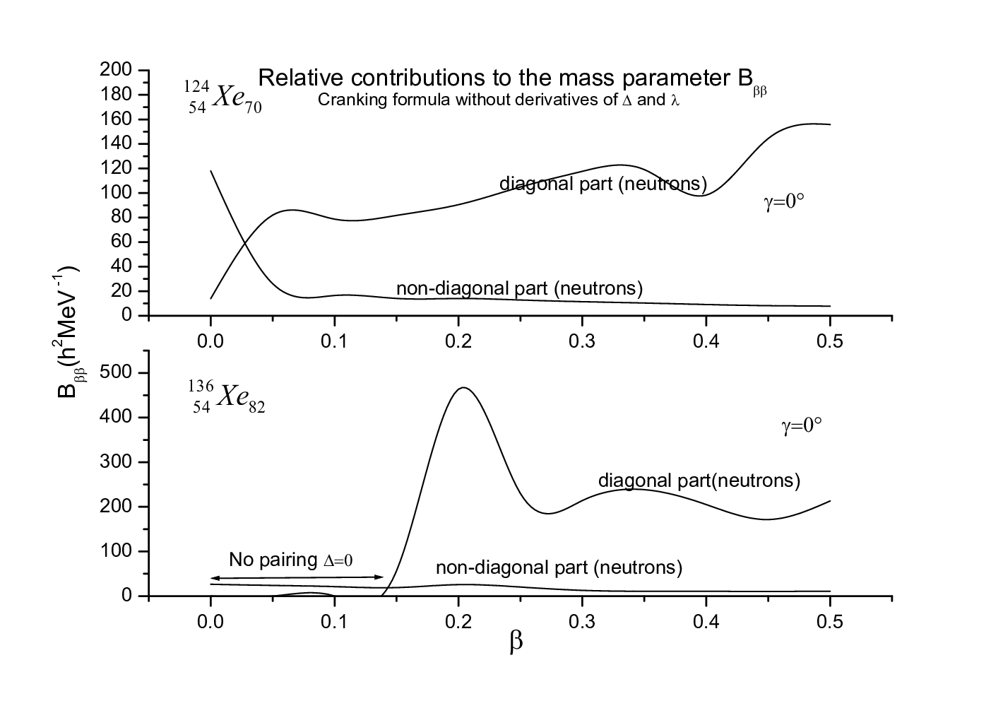
At this stage, the effects of the ”perturbations” involved by the derivatives are known. Therefore, from now, we will concentrate only on the formula of the cranking without derivatives. It is interesting to compare the magnitude of the contributions of the diagonal and non-diagonal parts given by Eq. (37). These two contributions are plotted in fig. 2 for a magic number of neutrons $N=82$ (bottom) and for a mid-shell neutron number $N=70$ (top). In the both cases, the diagonal contribution is dominant (about 10 times larger) if we except the region of the spherical shape ($\beta=0$) for $N=70$ which seems to be very particular.

Apart from the noted special spherical case, the explanation of these results can be easily understood. Indeed, first, the diagonal matrix elements are always by far more important than the other because in the integrand the derivative of the potential are multiplied by a squared wave function,

whereas for the non-diagonal matrix elements, i.e., for

the two radial wave functions are not always in phase, their product $\varphi_{\nu}^{\ast}(\overrightarrow{r},\beta,\gamma)\varphi_{\mu}(\overrightarrow{r},\beta,\gamma)$ has not a definite sign, the contributions to the integral will have tendency to cancel each other, or at least to lead to a small values.
It is clair that the more important coefficients $c_{\nu\mu}$ (diagonal and non diagonal) are those which are the closest to the Fermi level. Indeed, these coefficients are which given by (see Eq. (40)), are maximums when the quasiparticle energy $E_{\nu}=\sqrt{\left(\epsilon_{\nu}-\lambda\right)^{2}+\Delta^{2}}$ reaches its minimal value, i.e. for $\epsilon_{\nu}\approx\epsilon_{\mu}\approx\lambda$. The few important non-diagonal coefficients are generally multiplied by weak matrix elements. Indeed, for closed levels ($\nu\approx\mu,$ $\nu\neq\mu$), the radial wave functions are often in ”opposite” phase (like two ”consecutives” wave functions of the one dimensional infinite square well) so that the contribution to the integral will be necessarily very small. This explains why the diagonal part is dominant.
Before closing this paragraph, we would like to add an important remark concerning the shell effects. The latter are of course due to quantum mechanics. They involve sudden variations in the mass parameters with the number of particles. They appear when a few states contribute essentially to the mass parameters. In fact, for the mass parameters, we have a very limited number of diagonal matrix elements which contribute essentially to the mass parameters opposed to an admixture of a large number of small non-diagonal matrix elements. Consequently, it is clear that the shell effects will be contained in the diagonal part (of course without the derivatives).

We have found numerically that when there is not BCS solution the diagonal term (without derivatives) is practically equal to zero ($\sim 10^{-6}MEV$) so that the mass parameters reduce only to the non-diagonal part of the formula. In this case the mass parameters are very small. Because the values and the fluctuations of the mass parameters are mostly due to the diagonal contribution, our numerical study will concern exclusively this term. In the following, once more, we will concentrate obviously on the version of the formula without derivatives. The ”simple” diagonal part can be cast under the following form:

with,

As mentioned before, only few (about two up to five at all) energy levels contribute really to the final value of the mass parameters. Indeed, this function is peaked at $\lambda$ and due to the power of the denominator of Eq. (44) decreases very rapidly so that only few levels give important coefficients. For a valid BCS solution, a relative weak value of $\Delta$ gives significant coefficient $c_{\nu\nu}$.For example, we give in fig. 3 (bottom and top) the coefficients $c_{\nu\nu}$ (black stars) and the square of the matrix elements $\left\langle\nu\right|\partial V/\partial\beta_{i}\left|\nu\right\rangle^{2}$ (black squares) for the neutron contributions of the same two isotopes as before and the same deformation. First of course, we especially can check that these coefficients are important near the Fermi level ($41^{th}$ and $35^{th}$level). We have thus computed the four major neutron contributions of the energy levels and we have found $97\%$ and $82\%$ respectively for $N=82$ and $N=70$ cases. These contributions are not only due to the strongest values of the coefficients $c_{\nu\nu}$ but also to the ”corresponding” matrix elements (see Eq. (43)).We also can see very clearly the shell structure of the squared matrix elements which is the same for these two cases (because the deformation and hence the spectrum are the same in the both cases).

An other remark is that the maxima of the matrix elements are situated at the levels N${{}^{\circ}}15,25,41,65$ which correspond to the nucleon numbers $30,50,82,130$ which are magic or nearly magic, but these numbers are obtained for a weak deformed shape of the nucleus, whereas in the binding energy they match the spherical shape. Moreover these maxima are immediately preceded or followed by small values. Thus the shell structure of the matrix elements appears less regular than the one of the energy levels. As we can see, the shell structure is ”contained” not only in the level density but also in the matrix elements. Thus the mass parameters are characterized by a complex ”dual” shell structure.
At last, as a special case, we must point out the very strong values of the coefficients (i.e., the stars) in Fig 3-bottom involving very large the mass parameters at $\beta=0.2$. This very exceptional situation arises in the so called one crossing levels (see Ref.([11]) and ([12])) near the Fermi energy. This will be analyzed in the next subsection.

In Fig. 4, we have plotted the energy levels for different values of the deformation parameter $\beta$ ($\gamma$ being fixed to $0$). The BCS Fermi level is indicated by a star. This level is situated in the middle of a gap constituted by the last filled and the first unfilled levels. As $\beta$ increases, these two levels approach little by little each other. From the first $\left(\beta=0\right)$ and up to the fourth deformation $\left(\beta=0.2\right)$, the Fermi level lies always in the middle of a gap corresponding to the neutrons magic number $N=82$.

In these locations, the level density is so small with respect to the pairing strength so that it (i.e., the level density) is not able to insure a valid (non-trivial) BCS solution. In these four cases we have thus $\Delta\approx 0.0044$ $MEV$ and hence no valid BCS solution. Therefore, due to the weakness of $\Delta$, the diagonal term of (37) does not contribute at all to the mass parameters. In these situations, the mass parameters are very small ( $\sim 25\hbar^{2}$ $MEV^{-1}$in our case). However, for the deformation $\beta=0.2$, the two levels become very close to the Fermi level. It occurs in the immediate vicinity of the Fermi level a crossing levels. This happens inside a gap and gives rise to two very strong coefficients. Moreover, the corresponding values of the squared matrix elements are also important, giving practically all the contribution to the mass parameters. This phenomenon is characteristic of a phase transition (compare with 1-bottom). The remaining cases ($\beta$ beyond $0.25$) can be considered as ”normal cases”. They correspond to values about $c_{\nu\nu}\approx 0.1-0.2$.

We have focused our discussion around the mass parameter $D_{\beta\beta}$, but similar studies will lead to analog general conclusions (seen above) for the two other mass parameters $D_{\gamma\gamma}$ and $D_{\beta\gamma}$. However, we will make further useful remarks. For the quadrupole deformation $(\beta,\gamma)$, we write the detailed form for the three mass parameters (naturally, once more without the derivatives):

with $c_{\nu\mu}$ given by Eq. (40).
It is easy to compare these three quantities. First it is to be noted that they have the same coefficient so that the only difference will come from the matrix elements. The latter have not a definite sign in such a way that the third mass parameters will be the result of the sum of positive as well as negative terms. It will be thus necessary smaller than the two first mass parameters for which we have only positive contributions. Moreover, it is found numerically that $D_{\beta\beta}$ is generally larger than $D_{\gamma\gamma}.$ This can also be easily explained by the fact that the single-particle potential is generally more sensitive to the $\beta$ degree of freedom than the $\gamma$’s one, especially for the region the Barium isotopes. In other words for the quadrupole deformations and a Woods-Saxon potential we have,

Although the present work is devoted exclusively to the mass parameters, we would like to add an important remark concerning the moments of inertia. Indeed, these quantities can also be evaluated with the help of the cranking approximation including pairing correlations.(49):

Because the latter looks like to the one of the mass parameter (of course without the derivatives), it is tempting to conclude that the behaviour of these two quantities will in principle be the same. However, it is well known that unlike the mass parameters, the behaviour of the moments of inertia is always found as a smooth function of particle-number. It depends mainly on the deformation of the nucleus. This means that contrarily to the mass parameters, there are no shell effects in the moments of inertia. From our previous study, it is easy to interpret this difference.

First, this is due partly to the lower power of the denominator of Eq. (49) but the main reason is that there is no diagonal contribution ($\nu=\mu$) to this sum because the ”coefficient” vanishes when $\nu=\mu$. Remembering that the shells effects come almost exclusively from the diagonal part of the total contribution, we can conclude here that they will be necessary quasi absent in the moments of inertia.

References

• [1] M. Brack, J. Damgaard, A. S. Jensen, H. C. Pauli, V. M. Strutinsky and C. Y. Wong, Rev Mod. Phys. 44 (1972) 320
• [2] L. Prochniak, K. Zajac, K. Pomorski, S. G. Rohozinski, J. Srebrny, Nucl. Phys. A648, 181 (1999)
• [3] D. R. Inglis, Phys. Rev. 96 (1954) 1059, 97 (1955) 701
• [4] M. Baranger, M. Vénéroni, Ann. Phys. (NY) 114, 123 (1978).
• [5] M.J. Giannoni, P. Quentin, Phys. Rev. C21, 2060 (1980).
• [6] M.J. Giannoni, P. Quentin, Phys. Rev. C21, 2076 (1980).
• [7] S. T. Belyaev, Mat. Fys. Medd. Dan. Vid. Sehk. 31 (1959) N∘11
• [8] D. Bes, Mat. Fys. Medd. Dan. Vid. Selsk. 33 (1961) no. 2
• [9] B. Mohammed-Azizi, and D.E. Medjadi, Computer physics Comm. 156(2004) 241-282.
• [10] B. Mohammed-Azizi, and D.E. Medjadi, J. Phys. G : Nucl. Part. Phys. 35 (2008) 035101
• [11] J. J. Griffin, Nucl. Phys. A170 (1971) 395
• [12] T Ledergerber, H. C. Pauli, Nucl. Phys. A207 (1973) 1–32
• [13] P.-G. Reinhard, Nucl. Phys. A281 (1977) 221–239
• [14] D. N. Poenaru, R. A. Gherghescu, W. Greiner, Rom. Journ. Phys., Vol. 50, Nos. 1–2, P. 187–197, Bucharest, 2005
• [15] V. Schneider, J. Maruhn, and W. Greiner, Z. Phys. A 323 (1986) 111
• [16] Shan-Gui Zhou, Chunkai Zheng, and Jimin Hu, Phys. Rev. C63 (2001) 047305
• [17] J. Libert and P. Quentin, Z. Phys. A 306 (1982) 315