The 2009 World Average of
Abstract
Measurements of , the coupling strength of the Strong Interaction between quarks and gluons, are summarised and an updated value of the world average of is derived. Building up on previous reviews, special emphasis is laid on the most recent determinations of . These are obtained from -decays, from global fits of electroweak precision data and from measurements of the proton structure function , which are based on perturbative QCD calculations up to ; from hadronic event shapes and jet production in annihilation, based on QCD; from jet production in deep inelastic scattering and from decays, based on QCD; and from heavy quarkonia based on unquenched QCD lattice calculations. Applying pragmatic methods to deal with possibly underestimated errors and/or unknown correlations, the world average value of results in α_s(M_Z^0)= 0.1184 ±0.0007 . The measured values of , covering energy scales from GeV to 209 GeV, exactly follow the energy dependence predicted by QCD and therefore significantly test the concept af Asymptotic Freedom.
pacs
12.38.Qkexperimental tests of QCD1 Introduction
Quantum Chromodynamics (QCD) is the gauge field theory of the Strong Interaction [1]. QCD describes the interaction of quarks through the exchange of massless vector gauge bosons, the gluons, using concepts as known from Quantum Electrodynamics, QED. QCD, however, is more complex than QED because gluons themselves, other than photons in QED, carry the quantum-“ charge” of the Strong Interaction, such that gluons interact with each other.
As a consequence of the gluon self-coupling, QCD implies that the coupling strength , the analogue to the fine structure constant in QED, becomes large at large distances or - equivalently - at low momentum transfers 11 1 “Large” distances correspond to 1 fm, “low” momentum transfers to 1 GeV/c.. Therefore QCD provides a qualitative reason for the observation that quarks do not appear as free particles, but only exist as bound states of quarks, forming hadrons like protons, neutrons and pions. Hadrons appear to be neutral w.r.t. the strong quantum charge. The quark statistics of all known hadrons, their production cross sections and decay times imply that there are three different states of the strong charge.
In loose analogy to the behaviour of optical colours, the strong charge and the corresponding new quantum number is called “colour charge”. Quarks carry one out of three different colour charges, while hadrons are colourless bound states of 3 quarks or 3 antiquarks (“baryons”), or of a quark and an anti-quark (“mesons”). Gluons, in contrast to photons which do not carry (electrical) charge by themselves, have two colour charges.
QCD does not predict the actual of , however it definitely predicts the functional form of the of . While an increasingly large coupling at small energy scales leads to the “confinement” of quarks and gluons inside hadrons, the coupling becomes small at high-energy or short-distance reactions; quarks and gluons are said to be “asymptotically free”, i.e. 0 for momentum transfers .
The of , at a given energy or momentum transfer scale22 2 Here and in the following, the speed of light and Planck’s constant are set to unity, , such that energies, momenta and masses are given in units of GeV. , must be obtained from experiment. Determining at a specific energy scale is therefore a fundamental measurement, to be compared with measurements of the electromagnetic coupling , of the elementary electric charge, or of the gravitational constant. Testing QCD, however, requires the measurement of over ranges of energy scales: one measurement fixes the free parameter, while the others test the specific QCD prediction of confinement and of asymptotic freedom.
In this review the current status of measurements of is summarised. Theoretical basics of QCD and of the predicted energy dependence of are given in Section 2. Actual measurements of are presented in Section 3. A global summary of these results and a determination of the world average value of are presented in Section 4. Section 5 concludes and gives an outlook to future requirements and developments.
2 Theoretical basics
The concepts of Quantum Chromodynamics are presented in a variety of text books and articles, as e.g. [2, 3, 4, 5, 6, 7], such that in the following, only a brief summary of the basics of perturbative QCD and the running coupling parameter will be given.
2.1 Energy dependence of
With the value of known at a specific energy scale , its energy dependence is given by the renormalisation group equation
| (1) |
The perturbative expansion of the function is calculated to complete 4-loop approximation [8]:
| (2) | |||||
where
| (3) |
and is the number of active quark flavours at the energy scale . The numerical constants in equation 3 are functions of the group constants and , for theories exhibiting symmetry. For QCD and , and .
A solution of equation 1 in 1-loop approximation, i.e. neglecting and higher order terms, is
| (4) |
Apart from giving a relation between the values of at two different energy scales, at which is assumed to be known, and being another scale for which is being predicted, equation 4 also demonstrates the property of asymptotic freedom: if becomes large and is positive, i.e. if , will asymptotically decrease to zero for .
Likewise, equation 4 indicates that grows to large values and diverges to infinity at small : for instance, with and for typical values of , exceeds unity for . Clearly, this is the region where perturbative expansions in are not meaningful anymore. Therefore energy scales below the order of 1 GeV are regarded as the nonperturbative region where confinement sets in, and where equations 1 and 4 cannot be applied.
Including and higher order terms, similar but more complicated relations for , as a function of and of as in equation 4, emerge. They can be solved numerically, such that for a given value of , choosing a suitable reference scale like the mass of the boson, , can be accurately determined at any energy scale .
With
a dimensional parameter is introduced such that equation 4 transforms into
| (5) |
Hence, the parameter is technically identical to the energy scale where diverges to infinity. To give a numerical example, GeV for = 0.12 and = 5.
In complete 4-loop approximation and using the -parametrisation, the running coupling is given [9] by
| (6) | |||||
where . The first line of equation 6 includes the 1- and the 2-loop coefficients, the second line is the 3-loop and the third and the fourth lines denote the 4-loop correction, respectively.
The functional form of , in 4-loop approximation and for 4 different values of , is diplayed in figure 1. The slope and dependence on the actual value of is especially pronounced at small , while at large both the energy dependence and the dependence on becomes increasingly feeble.

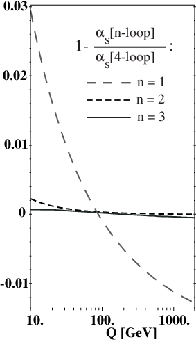
The relative size of higher order loop corrections and the degree of convergence of the perturbative expansion of is demonstrated in figure 2, where the fractional difference in the energy dependence of , , for = 1, 2 and 3, is presented. The values of were chosen such that in each order, i.e., MeV (1-loop), MeV (2-loop), and MeV (3- and 4-loop). Only the 1-loop approximation shows sizeable differences of up to several per cent, in the energy and parameter range chosen, while the 2- and 3-loop approximations already reproduce the energy dependence of the 4-loop prediction quite accurately.
The parametrisation of the running coupling with instead of has become a common standard, see e.g. [6]. It will also be adopted here.
2.2 Quark threshold matching
Physical observables , when expressed as a function of , must be continuous when crossing a quark threshold where changes by one unit. This determines that actually depends on the number of active quark flavours. will therefore be labelled to indicate these peculiarities. Also the slope of the energy dependence and, in approximations higher than 2-loop, the value of change at the quark thresholds:
Construction of theoretical predictions which consistently match at a quark flavour threshold leads to matching conditions for the values of above and below that threshold [10]. In leading and in next-to-leading order, the matching condition is . In higher orders, however, nontrivial matching conditions apply [9, 10, 11]. Formally these are, if the energy evolution of is performed in order (or loops), of order ().
The matching scale can be chosen in terms of the (running) mass , or of the constant, so-called pole mass . For both cases, the relevant matching conditions are given in [9]. These expressions have a particluarly simple form for the choice33 3 The results of reference [9] are also valid for other relations between and or , as e.g. . For 3-loop matching, differences due to the freedom of this choice are negligible. or . In this review, the latter choice will be used to perform 3-loop matching at the heavy quark pole masses, in which case the matching condition reads, with and :
| (7) |
where and [9].
The fractional difference of the 4-loop prediction for the running , using equation 6 with = 213 MeV and 3-loop matching at the charm- and bottom-quark pole masses, GeV and GeV, and the 4-loop prediction without applying matching and with = 5 throughout are illustrated in figure 3. Small discontinuities at the quark thresholds can be seen, such that by about 2 per mille at the bottom- and about 1 per cent at the charm-quark threshold. The corresponding values of are MeV and MeV. In addition to the discontinuities, the matched calculation shows a steeper rise towards smaller energies because of the larger values of and . Note that the step function of is not an effect which can be measured; the steps are artifacts of the truncated perturbation theory and the requirement that predictions for observables at energy scales around the matching point must be consistent and independent of the two possible choices of (neighbouring) values of .

2.3 Perturbative predictions of physical quantities
In perturbative QCD, physical quantities are usually given by a power series in , like
| (8) | |||||
where are the order coefficients of the perturbation series and denotes the lowest-order value of . is the leading order (LO) coefficient, is called the next-to-leading order (NLO), is the next-to-next-to-leading order (NNLO) and the N3LO coefficient.
QCD calculations in NLO perturbation theory are available for many observables in high energy particle reactions like hadronic event shapes, jet production rates, scaling violations of structure functions. Calculations including the complete NNLO are available for some totally inclusive quantities, like the total hadronic cross section in , moments and sum rules of structure functions in deep inelastic scattering processes, the hadronic decay widths of the boson and of the lepton. More recently, NNLO predictions were provided for exclusive quantities like hadronic event shape distributions and differential jet production rates in annihilation [12], and N3LO predictions for the hadronic width of the boson and the lepton [13] became available.
A further approach to calculating higher order corrections is based on the resummation of logarithms which arise from soft and collinear singularities in gluon emission [14]. Application of resummation techniques and appropriate matching with fixed-order calculations are further detailed e.g. in [7].
2.4 Renormalisation
In quantum field theories like QCD and QED, physical quantities can be expressed by a perturbation series in powers of the coupling parameter or , respectively. If these couplings are sufficiently small, i.e. if , the series may converge sufficiently quickly such that it provides a realistic prediction of even if only a limited number of perturbative orders will be known.
In QCD, examples of such quantities are cross sections, decay rates, jet production rates or hadronic event shapes. Consider being dimensionless and depending on and on a single energy scale . When calculating as a perturbation series of a pointlike field theory in , ultraviolet divergencies occur. These divergencies are removed by the “renormalisation” of a small set of physical parameters. Fixing these parameters at a given scale and absorbing this way the ultraviolet divergencies, introduces a second but artificial momentum or energy scale . As a consequence of this procedure, and become functions of the renormalisation scale . Since is dimensionless, we assume that it only depends on the ratio and on the renormalized coupling :
Because the choice of is arbitrary, however, the actual value of the experimental observable cannot depend on , so that
| (9) |
where the derivative is multiplied with in order to keep the expression dimensionless. Equation 9 implies that any explicite dependence of on must be cancelled by an appropriate -dependence of to all orders. It would therefore be natural to identify the renormalisation scale with the physical energy scale of the process, , eliminating the uncomfortable presence of a second and unspecified scale. In this case, transforms to the “running coupling constant” , and the energy dependence of enters only through the energy dependence of .
The principal independence of a physical observable from the choice of the renormalisation scale was expressed in equation 9. Replacing by , using equation 1, and inserting the perturbative expansion of (equation 8) into equation 9 results, for processes with constant , in
| (10) | |||||
Solving this relation requires that the coefficients of vanish for each order . With an appropriate choice of integration limits one thus obtains
| (11) | |||||
as a solution of equation 10.
Invariance of the complete perturbation series against the choice of the renormalisation scale therefore implies that the coefficients , except and , explicitly depend on . In infinite order, the renormalisation scale dependence of and of the coefficients cancel; in any finite (truncated) order, however, the cancellation is not perfect, such that all realistic perturbative QCD predictions include an explicit dependence on the choice of the renormalisation scale.
The scale dependence is most pronounced in leading order QCD because does not explicitly depend on and thus, there is no cancellation of the (logarithmic) scale dependence of at all. Only in next-to-leading and higher orders, the scale dependence of the coefficients , for , partly cancels that of . In general, the degree of cancellation improves with the inclusion of higher orders in the perturbation series of .
Renormalisation scale dependence is often used to test and specify uncertainties of theoretical calculations for physical observables. In most studies, the central value of is determined or taken for equalling the typical energy of the underlying scattering reaction, like e.g. in annihilation. Changes of the result when varying this definition of within “reasonable ranges” are taken as systematic higher order uncertainties.
There are several proposals of how to optimise or fix the renormalisation scale, see e.g. [15, 16, 17, 18] Unfortunately, there is no common agreement of how to optimise the choice of scales or how to define the size of the corresponding uncertainties. This unfortunate situation should be kept in mind when comparing and summarising results from different analyses.
In next-to-leading order, variation of the renormalisation scale is sufficient to assess and include theoretical uncertainties due to the chosen renormalisation scheme and the limited (truncated) perturbation series. In NNLO and higher, howerer, the renormalisation scale and the renormalisation scheme should be varied for a complete assessment. While it has become customary to include renormalisation scale variations when applying theoretical predictions, changes of the renormalisation scheme are rarely explored. Instead, the so-called “modified minimal subtraction scheme” () [19] is commonly used in most analyses, which is also the standard choice in this review.
2.5 Nonperturbative methods
At large distances or low momentum transfers, becomes large and application of perturbation theory becomes inappropriate. Nonperturbative methods have therefore been developed to describe strong interaction processes at low energy scales of typically GeV2, such as the fragmentation of quarks and gluons into hadrons (“hadronisation”) and the masses and mass splittings of mesons.
Hadronisation models are used in Monte Carlo approaches to describe the transition of quarks and gluons into hadrons. They are based on QCD-inspired mechanisms like the “string fragmentation” [20, 21] or “cluster fragmentation” [22], and are usually implemeted, together with perturbative QCD shower and/or (N)LO QCD generators, in models describing complete hadronic final states in high energy particle collisions. Those models contain a number of free parameters which must be adjusted in order to reproduce experimental data well. They are indispensable tools not only for detailed QCD studies of high energy collision reactions, but are also important to assess the resolution and acceptance of large particle detector systems.
Power corrections are an analytic approach to approximate nonperturbative hadronisation effects by means of perturbative methods, introducing a universal, non- perturbative parameter
to parametrise the unknown behaviour of below a certain infrared matching scale [23]. Power corrections are regarded as an alternative approach to describe hadronisation effects on event shape distributions, instead of using phenomenological hadronisation models.
Lattice Gauge Theory is one of the most developed nonperturbative methods (see e.g. [24]) and is used to calculate, for instance, hadron masses, mass splittings and QCD matrix elements. In Lattice QCD, field operators are applied on a discrete, 4-dimensional Euclidean space-time of hypercubes with side length . Finite size lattice and spacing effects are studied by using increasing lattice sizes and decreasing lattice spacing , hoping to eventually approach the continuum limit. With ever increasing computing power and refined Monte Carlo methods, these calculations significantly matured over time and recently provided predictions of the proton (and other hadron) masses to better than 2% [25], and determinations of from quarkonia mass splittings with a precision of better than 1 % [26].
3 Measurements of
Since almost 30 years, determinations of continue to be at the forefront of experimental studies and tests of QCD. Increasing precision of QCD predictions and methods, improved understanding and parametrisation of non- perturbative effects, increased data quality and statistics and the availabilty of data over large ranges of energy and from a large variety of processes have led to an ever increasing precision and depth of these studies. The timely development of determinations was documented and summarised in a number of summary articles, see e.g. [27, 7, 6, 28], on which this review is intended to build up. Since about the year 2000, the precision of determinations and the multitude of results from various processes and ranges of energies provided experimental proof [7, 28] of the concept of asymptotic freedom.
In this review, special emphasis is laid on an update of the review from 2006 [28], concentrating on the most recent results which are mostly based on further improved theoretical predictions and/or experimental precision:
- •
perturbative QCD predictions in complete N3LO for the hadronic widths of the boson and the lepton are now available, improving further the completeness of the perturbative series and providing increased control of remaining theoretical uncertainties;
- •
improved lattice QCD simulations with vacuum polarisation from u, d and s quarks, updating previous determinations of and quoting overall uncertainties of less than 1%;
- •
an improved extraction of from radiative decays of the (1s);
- •
a combined analysis of non-singlet structure functions from deep inelastic scattering data, based on QCD predictions complete to N3LO;
- •
a combined analysis of inclusive jet cross section measurements in neutral current deep inelastic scattering at high ;
- •
determinations of from hadronic event shapes and jet rates in annihilation final states, an important and (experimentally) very precise environment, based on the new and long awaited QCD predictions in complete NNLO QCD.
These recent results are superior to and thus replace a large number of determinations published before 2006 and summarised in [28]. While those previous measurements still remain valid, only the new results listed above are presented and summarised below.
3.1 from -lepton decays
Determination of from lepton decays is one of the most actively studied fields to measure this basic quantity. The small effective energy scale, GeV, small nonperturbative contributions to experimental measurements of a total inclusive observable, the normalised hadronic branching fraction of lepton decays,
invariant mass distributions (spectral functions) of hadronic final states of -decays, and the “shrinking error” effect of the QCD energy evolution of towards higher energies 44 4 According to equations 1 and 2, in leading order, . Therefore, since decreases by about a factor of 3 when running from to , the relative error of also decreases by about a factor of 3. provide the means for one of the most precise determinations of . Theoretically, is predicted to be [29]
| (12) |
Here, [30] and [31] are electroweak corrections, [6], and are perturbative and nonperturbative QCD corrections. Most recently, was calculated to complete N3LO perturbative order, [13]; it is of similar structure as the one for the hadronic branching fraction of the boson. Based on the operator product expansion (OPE) [32], the nonperturbative corrections are estimated to be small [29], . A comprehensive review of the physics of hadronic decays was given in [33].
Recently, several authors have revisited the determination of from decays [13, 34, 35, 36, 37, 38]. These studies are based on data from LEP [39] and - partly- from BABAR [40]. They differ, however, in the detailed treatment and usage of the perturbative QCD expansion of . In particular, the usage of either fixed order (FOPT) or contour improved perturbative expansion (CIPT), and differences in the treatment and inclusion of nonperturbative corrections, leads to systematic differences in the central values of , ranging from 0.316 to 0.344, as summarised in figure 4. Results based on FOPT turn out to be systematically lower than those using CIPT - a trend being known for quite some time, and being actively disputed in the literature, but not finally being solved.

The results shown in figure 4, within their assigned total uncertainties, are partly incompatible with each other. This is especially true if considering that they are based on the same data sets. The main reason for these discrepancies is the usage of either the FOPT or the CIPT pertubative expansions. Note that only the result of Baikov et al. [13] averages between these two expansions, and assigns an overall error which includes the difference between these two.
In view of these differences and for the sake of including the apparent span between different perturbative expansions in the overall error, the range shown as shaded band in figure 4 and the corresponding central value is taken as the final result from -decays, leading to
Running this value to the rest mass of 91.2 Ge,V using the 4-loop solution of the -function (equation 6) with 3-loop matching at the heavy quark pole masses GeV and GeV, results in
This value will be included in determining the world average of as described in section 4.
3.2 from heavy quarkonia
Heavy Quarkonia, i.e. meson states consisting of a heavy (charm- or bottom-) quark and antiquark, are a classical testing ground for QCD, see e.g. [41]. Masses, mass splittings between various states, and decay rates are observables which can be measured quite accurately, and which can be predicted by QCD based on both perturbation theory and on lattice calculations.
3.2.1 from radiative decays
Bound states of a bottom quark and antiquark are potentially very sensitive to the value of because the hadronic decay proceeds via three gluons, hadrons. The lowest order QCD term (i.e. in equation 8) for the hadronic decay width already contains to the power. The situation is more complicated, however, due to relativistic corrections and to the unknown wave function of the at the origin.
The wave function and relativistic corrections largely cancel out in ratios of decay widths like
which therefore are the classical observables for precise determinations of .
In [42], recent CLEO data [43] are used to determine from radiative decays of the (1S). The theoretical predictions include QCD up to NLO. They are based on recent estimates of colour octet operators and avoid any model dependences. The value obtained from this study is
It is compatible with previous results from similar studies, see e.g. [7, 28] and references quoted therein. It will be included in the calculation of the new world average of .
3.2.2 from lattice QCD
Determinations of based on lattice QCD calculations have become increasingly inclusive and precise in the past, including light quarks (u,d and s) in the vacuum polarisation and incorporating finer lattice spacing.
In a recent study by the HPQCD collaboration [26], the QCD parameters - the bare coupling constant and the bare quark masses - are tuned to reproduce the measured ’ - meson mass difference. The u, d and s quark masses are adjusted to give correct values of various light meson masses. With these parameters set, there are no other free physical parameters, and the simulation is used to provide accurate QCD predictions. Nonperturbative values of several short-distance quantities are computed and compared to respective perturbative calculations which are given in NNLO perturbation theory. From a fit to 22 short distance quantities, the value of
is finally obtained. The total error incudes finite lattice spacing, finite lattice volume, perturbative and extrapolation uncertainties. This result will be an important ingredient of the new world average determined in section 4.
3.3 from deep inlastic scattering
Measurements of scaling violations in deep inelastic lepton-nucleon scattering belong to the earliest methods used to determine . The first significant determinations of , being based on perturbative QCD prediction in NLO, date back to 1979 [44].
Today, a large number of results is available from data in the energy () range of a few to several thousand GeV2, using electron-, muon- and neutrino-beams on various fixed target materials, as well as electron-proton or positron-proton colliding beams at HERA. In addition to scaling violations of structure functions, is also determined from moments of structure functions, from QCD sum rules and — similar as in annihilation — from hadronic jet production and event shapes. Improved QCD predictions as well as new experimental studies provided new results from a combined study of world data on structure functions, and from jet production at HERA.
3.3.1 from world data on non-singlet structure functions
Physical processes in lepton-nucleon and in hadron-hadron collisions depend on quark- and gluon-densities in the nucleon. Assuming factorisation between short-distance, hard scattering processes which can be calculated using QCD perturbation theory, and low-energy or long-range processes which are not accessible by perturbative methods, such cross sections are parametrised by a set of structure functions (= 1,2,3).
The energy dependence of structure functions is given by perturbative QCD. A study [45] of the available world data on deep inelastic lepton-proton and lepton-deuteron scattering provided a determination of the valence quark parton densities and of in wide ranges of the Bjorken scaling variable and . In the non-singlet case, where heavy flavour effects are negligibly small, the analysis is extended to 4-loop level, i.e. to QCD in N3LO perturbative expansion.
The determination of to this level results in
where the total error includes a theoretical uncertainty of which is taken from the difference between the N3LO and the NNLO result. This value will be included in the determination of the world average of .
As it appears, fits of in determinations of parton density functions from purely deep inelastic scattering processes result in somewhat smaller values than those which also include hadron collider data, see e.g. [46] obtaining . They also are systematically smaller than the world average value of , see below.
3.3.2 from jet production in deep inelastic scattering processes
Measruements of from jet production in deep inelastic lepton- nucleon scattering at the HERA collider have been and continue to be an active field of research. Inclusive as well as differential jet production rates were studied in the energy range of up to 15000 GeV2, based on similar jet definitions and algorithms as used in annihilation.
In a recent summary and combination [47] of precision measurements at HERA, values of where determined from fits of NLO QCD predictions to data of inclusive jet cross sections in neutral current deep inelastic scattering at high [48, 49]. The overall combined result,
has a reduced theoretical uncertainty of (added in quadrature to the experimental error of ) compared to previous combinations, due to carefully selected ranges of data in ranges where theoretical uncertainties are minimal [47]. This combined result will be included in the determination of the world average of .
3.4 from hadronic event shapes and jet production in annihilation
Observables parametrizing hadronic event shapes and jet production rates are the classical inputs for studies in annihilation. The measurements summarised in previous reviews [7, 50, 51, 28] were based on QCD predictions in NLO, which partly included summation of next-to-leading logarithms (NLLA) to all orders. As one of the most notable and long awaited theoretical improvements, complete NNLO predictions became available recently [12], which are also matched with leading and next-to-leading logarithms resummed to all orders [52] (NNLO + NLLA).
The advancement in theoretical descriptions was instantly used to determine from data of previous annihilation experiments, from the PETRA and the LEP colliders which operated from 1979 to 1986 and from 1989 to 2000, respectively. The usage of data of past experiments demonstrates the need to preserve data as well as reconstruction-, simulation- and analysis-software for a time-span significantly exceeding the usual -year period of post-data taking analysis.
A re-analysis [53] of the ALEPH data from LEP, in the c.m. energy range from 90 to 206 GeV, based on six event shape and jet production observables, results in
The total error contains an experimental uncertainty of 0.0013 and a theoretical uncertainty, mainly from hadronisation and from renormalisation scale dependences, of 0.0037. This result is obtained using NNLO+NLLA QCD predictions; in NNLO alone, the central value is slightly higher (0.1240) and the total error is sligthly smaller (0.0032). NNLA terms, although they should provide a more complete perturbation series, tend to introduce somewhat larger scale uncertainties [53].
Similar results are available from a re-analysis of data from the JADE experiment at PETRA [54], from six event shape and jet observables at six c.m. energies in the c.m. energy range from 14 to 46 GeV:
The total error contains an experimental uncertainty of 0.0020 and a theoretical uncertainty of 0.0046. Also this result is obtained using QCD predictions in NNLO+NLLA; the value for NNLO alone is .
Both the NNLO+NLLA results from ALEPH and from JADE data are retained for the determination of the new world average value of in this review. Because they are based on data at different c.m. energy ranges and from two independent experiments, they add valuable and independent information not only on the world average, but also on the experimental verification of the running of . These two results of are included in figure 5; the respective values of , obtained at different values of c.m. energies, are displayed in figure 6.
Recently, the event shape observable thrust [55] was also studied from LEP data using methods of effective field theory [56]. Starting from a factorisation theorem in soft-collinear effective theory, the thrust distribution is calculated including resummation of the next-to-next-to-next-to-leading logarithms (N3LL). The result of this analysis is , whereby the error includes a theoretical uncertainty of . Although this is formally one of the smallest errors quoted on measurements of , this result is not explicitly included in the world average calculated below. The reason for this decision is two-fold: First, the LEP thrust data are already included in the re-analysis of ALEPH data described above. Second, this analysis based on effective field theory, although being a highly interesting, alternative approach to studies based on standard perturbation theory, is not yet in a state of comparable reliability because it is based on one event shape observable only, and therefore misses an important verification of potential systematic uncertainties.
3.5 from electroweak precision data
The determination of from totally inclusive observables, like the hadronic width of the lepton discussed above, or the total hadronic decay width of the boson, are of utmost importance because they lack many sources of systematic uncertainties, experimental as well as theoretical, which differential distributions like event shapes or jet rates suffer from. In this sense, the ratio of the hadronic to the leptonic partial decay width, , is a “gold plated” observable.
Since 1994, the QCD correction to is known in NNLO QCD [57]. The measured value from LEP, [58], results in , where the error is experimental. An additional theoretical uncertainty was estimated [7] as .
As already mentioned, the full N3LO prediction of , i.e. in perturbative expansion, is now available [13]. The negative term results in an increase of by 0.0005, such that the actual result from the measured value of is: Defining the remaining theoretical uncertainty as the difference between the NNLO and the N3LO result, the theory error would not visibly contribute any more, given the current size of the experimental error on of .
A more precise value of can be obtained from general fits to all existing electro-weak precision data, using data from the LEP and the SLC colliders as well as measurements of the top-quark mass and limits on the Higgs boson mass from Tevatron and LEP. Such global fits result in values of with reduced experimental errors. These values, however, were consistently smaller than (but still compatible with) the ones obtained from alone, see e.g. [58].
A recent revision of the global fit to electroweak precision data [59], based on a new generic fitting package [60], on the up-to-date QCD corrections in N3LO, on proper inclusion of the current limits from direct Higgs-searches at LEP and at the Tevatron and on other improved details, results in
where the first error is experimental and the second is theoretical, estimated by the difference of the results in NNLO and in N3LO QCD.
| Process | Q [GeV] | excl. mean | std. dev. | ||
|---|---|---|---|---|---|
| -decays | 1.78 | 0.9 | |||
| DIS [] | 2 - 15 | – | 1.7 | ||
| DIS [e-p jets] | 6 - 100 | – | 0.4 | ||
| states | 7.5 | 0.2 | |||
| decays | 9.46 | 0.1 | |||
| [jets & shps] | 14 - 44 | – | 0.2 | ||
| [ew] | 91.2 | 0.3 | |||
| [jets & shps] | 91 - 208 | – | 1.0 |
4 The 2009 world average of
The new results discussed in the previous section are summarised in table 1 and in figure 5. Since all of them are based on improved theoretical predictions and methods, and/or on improved data quality and statistics, they supersede and replace their respective precursor results which were summarised in a previous review [28]. While those previous results continue to be valid measurements, they are not discussed in this review again, and they will not be included in the determination of a combined world average values of , according to the following reasons:
- 1.
from each class of measurements, only the most advanced and complete analyses shall be included in the new world average;
- 2.
older measurements being complemented or superseded by the most recent results listed above, as e.g. results from sum rules, from singlet structure functions of deep inelastic scattering, and from jet production and b-quark production at hadron colliders, are not included because their relatively large overall uncertainties, in general, will not give them a sizable weight but will complicate the definition of the overall error of the combined value of ;
- 3.
restricting the new world average to the most recent and most complete (i.e. precise) results allows to examine the consistency between the newest and the previous generations of measurements and reviews.
4.1 Numerical procedure
The average of a set of different, uncorrelated measurements of a particular quantity with individual errors or uncertainties, is commonly defined using the method of (see e.g. [6]: For being independent and statistically distributed measures with a common expectation value but with different variances , the weighted average is defined by
| (13) |
and the variance of is minimised by choosing
| (14) |
The quality of the average is defined by the variable,
| (15) |
which is, for uncorrelated data, expected to be equal to the number of degrees of freedom, :
The results summarised in table 1, however, are not independent of each other. They are, in the most general sense, correlated to an unknown degree. While the statistical errors of the data and the experimental systematic uncertainties contained in the errors are independent and uncorrelated, the theoretical uncertainties are very likely to be (partly) correlated between different results, because they are all based on applying the same underlying theory, i.e. QCD, and similar methods to obtain estimates of theoretical uncertainties are being used.
For some observables, like e.g. the hadronic widths of the boson and the lepton, the theoretical predictions and hence, their uncertainties, are known to be correlated by almost 100%. For other cases, like the results based on lattice QCD and those based on QCD perturbation theory, it can be assumed that their theoretical uncertainties are not correlated at all. In addition to the inherent lack of knowledge of theoretical correlations, estimates of theoretical uncertainties, in general, are performed in widely different ways, using different methods and different ranges of parameters.
The presence of correlated errors, if using the equations given above, is usually signalled by . Values of , in most practical cases, are a sign of possibly underestimated errors. In this review, both these cases are pragmatically handled in the following way:
In the presence of correlated errors, described by a covariance matrix , the optimal procedure to determine the average is to minimise the function
which leads to
and
The choice of and for retains the uncorrelated case given above. In the presence of correlations, however, the resulting will be less than . In order to allow for an unknown degree of a correlation , the method proposed in [61] will be applied by choosing and adjusting such that .
For cases where the uncorrelated error determimation results in , and in the absence of knowledge which of the errors are possibly underestimated, all individual errors are scaled up by a common factor such that the resulting value of , using the definition for uncorrelated errors, will equal unity.
Note that both for values of or , increases, compared to the uncorrelated ( and ) case.

4.2 Determination of the world average
The eight different determinations of summarised and discussed in the previous section are listed in table 1 and are graphically displayed in figure 5. Applying equations 13, 14 and 15 to this set of measurements, assuming that the errors are not correlated, results in an average value of with .
The fact that signals a possible correlation between all or subsets of the eight input results. Assuming an overall correletion factor and demanding that requires , inflating the overall error from 0.00063 to 0.00089.
In fact, there are two pairs of results which are known to be largely correlated:
- •
the two results from event shapes based on the data from JADE and from ALEPH use the same theoretical predictions and similar hadronisation models to correct these predictions for the transitions of quarks and gluons to hadrons. While the experimental errors are uncorrelated, the theoretical uncertainties may be assumed to be correlated to 100%. The latter accounts for about 2/3 to 3/4 of the total errors. An appropriate choice of correlation factor between the two may then be .
- •
the QCD predictions for the hadronic widths of the -lepton and the boson are essentially identical, so the respective results on are correlated, too. The values and total errors of from decays must therefore be correlated to a large extend, too. In this case, however, the error of one measurement is almost entirely determined by the experimental error (-decays), while the other, from -decays, is mostly theoretical. A suitable choice of the correlation factor between both these results may thus be .
Inserting these two pairs of correlations into the error matrix , the of the averaging procedure results in 6.8/7, and the overall error on the (unchanged) central value of changes from 0.00063 to 0.00067. Therefore the new world average value of is defined to be
For seven out of the eight measurements of , the average value of 0.1184 is within one standard deviation of their assigned errors. One of the measurements, from structure functions [45], deviates from the mean value by more than one standard deviation, see figure 5.
The mean value of is potentially dominated by the result with the smallest overall assigned uncertainty, which is the one based on lattice QCD [26]. In order to verify this degree of dominance on the average result and its error, and to test the compatibility of each of the measurements with the others, exclusive averages, leaving out one of the 8 measurements at a time, are calculated. These are presented in the column of table 1, together with the corresponding number of standard deviations 55 5 The number of standard deviations is defined as the square-root of the value of . between the exclusive mean and the respective single measurement.
As can be seen, the values of exclusive means vary only between a minimum of 0.11818 and a maximum 0.11876. Note that in the case of these exclusive means and according to the ”rules” of calculating their overall errors, in four out of the eight cases small error scaling factors of had to be applied, while in the other cases, overall correlation factors of about 0.1, and in one case of 0.7, had to be applied to assure . Most notably, the average value changes to when omitting the result from lattice QCD.
5 Summary and Discussion
In this review, new results and measurements of are summarised, and the world average value of , as previously given in [7, 28, 6], is updated. Based on eight recent measurements, which partly use new and improved N3LO, NNLO and lattice QCD predictions, the new average value is
which corresponds to
This result is consistent with the one obtained in the previuos review three years ago [28], which was . The previous and the actual world average have been obtained from a non-overlapping set of single results; their agreement therefore demonstrates a large degree of compatibility between the old and the new, largely improved set of measurements.
The individual mesurements, as listed in table 1 and displayed in figure 5, show a very satisfactory agreement with each other and with the overall average: only one out of eight measurements exceeds a deviation from the average by more than one standard deviation, and the largest deviation between any two out of the eight results, namely the ones from decays and from structure functions, amounts to 2 standard deviations 66 6 assuming their assigned total errors to be fully uncorrelated..
There remains, however, an apparent and long-standing systematic difference: results from structure functions prefer smaller values of than most of the others, i.e. those from annihilations, from decays, but also those from jet production in deep inelastic scattering. This issue apparently remains to be true, although almost all of the new results are based on significantly improved QCD predictions, up to N3LO for structure functions, and hadronic widths, and NNLO for event shapes.
The reliability of “measurements” of based on “experiments” on the lattice have gradually improved over the years, too. Including vaccum polarisation of three light quark flavours and extended means to understand and correct for finite lattice spacing and volume effects, the overall error of these results significally decreased over time, while the value of gradually approached the world average. Lattice results today quote the smallest overall error on ; it is, however, ensuring to see and note that the world average lattice results is only marginally different, while the small size of the total uncertainty on the world average is, naturally, largely influenced by the lattice result.

In order to demonstrate the agreement of measurements with the specific energy dependence of predicted by QCD, in figure 6 the recent measurements of are shown as a function of the energy scale . For those results which are based on several determinations at different values of energy scales , the individual values of are displayed. For the value from structure functions such a breakup is not possible; instead, the corresponding result derived for a typical energy scale of GeV is displayed.
The measurements significantly prove the validity of the concept of asymptotic freedom; they are in perfect agreement with the QCD prediction of the running coupling. This is further corroborated by figure 7, where a selected sample of the measurements is plotted, now as a function of , in order to demonstrate the data reproducing the specific logarithmic shape of the running as predicted by QCD, signalling that indeed for .

What are the future prospects of measurements of ? With the given degree of data and theory precision, further improvements will be difficult and may take quite some time. Experimentally, a linear collider, especially if run in the “Giga-Z” mode, has the potential to decrease the dominating experimental error of from the measurement of , down and below its theoretical uncertainty which currently is assumed to be, in N3LO, .
While it is unlikely that QCD perturbation theory will improve to yet one order higher than the existing N3LO or NNLO predictions, improvements are likely, and actually are very neccessary, for QCD predictions of jet production in deep inelastic scattering and in hadron collisions, where calculations currently are limited to NLO. The precision of QCD tests, but also the sensitivity for observing new physics signals at the LHC, will largely depend on a further advancement of QCD predictions for hadron collisions.
Future improvement of theoretical predictions and models require the conservation of data and of reconstruction and simulation code of current and past experiments; especially in the case of deep inelastic scattering data, re-application of improved predictions and models carry a large potential for future advancements in this field.
Last but not least, further developments of non- perturbative methods are mandatory to bridge the gap between quarks and gluons and their final states, hadrons. They may in fact shed more light into the systematic differences between some classes of measurements as discussed above.
References
- (1)
H. Fritzsch, M. Gell-Mann and H. Leutwyler
Phys. Lett. B47, (1973) 365;
D.J. Gross, F. Wilczek, Phys. Rev. Lett. 30 (1973) 1343; Phys. Rev. D8 (1973) 3633;
H.D. Politzer, Phys. Rev. Lett. 30 (1973) 1346. - (2) R.K. Ellis, W.J. Stirling and B.R. Webber, QCD and Collider Physics, Cambridge University Press, 1996.
- (3) J.C. Collins, Renormalization, Cambridge University Press, 1984.
- (4) F.J. Yndurain, The Theory of Quark and Gluon Interactions, Springer-Verlag, 1999.
- (5) G. Dissertori, I.G. Knowles, M. Schmelling, High energy experiments and theory, Oxford, UK: Clarendon (2003) 538 p, (International series of monographs on physics. 115).
- (6) PDG, C. Amsler et al., Phys. Lett. B667 (2008).
- (7) S. Bethke, J. Phys. G26, (2000) R27; hep-ex/0004021.
- (8)
T. van Ritbergen, J.A.M. Vermaseren, S.A. Larin, Phys. Lett.
B400 (1997) 379.
M. Czakon, Nucl.Phys. B710 (2005) 485; hep-ph/0411261. - (9) K.G. Chetyrkin, B.A. Kniehl and M. Steinhauser, Phys. Rev. Lett. 79 (1997) 2184.
- (10) W. Bernreuther and W. Wetzel, Nucl. Phys. B197 (1982) 128.
- (11) S.A. Larin, T. van Ritbergen and J.A.M. Vermaseren, Nucl. Phys. B438 (1995) 278.
- (12)
A. Gehrmann-de Ridder et al., JHEP 0712 (2007) 094;
arXiv:0711.4711 [hep-ph].
S. Weinzierl, Phys. Rev. Lett. 101 (2008) 162001; arXiv:0807.3241 [hep-ph]. - (13) P.A. Baikov, K.G. Chetyrkin, J.H. Kühn, Phys. Rev. Lett. 101 (2008) 012002, arXiv:0801.1821 [hep-ph].
- (14) S. Catani, L. Trentadue, G. Turnock, B.R. Webber, Nucl. Phys. B407 (1993) 3.
- (15) P.M. Stevenson, Phys. Rev. D23 (1981) 2916.
- (16) G. Grunberg, Phys. Rev. D29 (1984) 2315.
- (17) S.J. Brodsky, G.P. Lepage and P.B. Mackenzie, Phys. Rev. D28 (1983) 228.
- (18) S. Bethke, Z. Phys C43 (1989) 331.
- (19) W.A. Bardeen et al., Phys. Rev. D18 (1978) 3998.
- (20) T. Sjostrand, Comput. Phys. Commun. 27 (1982) 243.
- (21) T. Sjostrand, S. Mrenna and P Skands, Comput.Phys.Commun. 178 (2008) 852; arXiv:0710.3820 [hep-ph].
- (22)
G. Marchesini and B.R. Webber, Nucl.Phys. B238 (1984) 1;
G. Corcella et al., JHEP 0101 (2001) 010, hep-ph/0011363. - (23)
Yu.L. Dokshitzer, B.R. Webber, Phys. Lett. B352 (1995) 451;
Yu.L. Dokshitzer, G. Marchesini, B.R. Webber, Nucl.Phys. B469 (1996) 93;
Yu.L. Dokshitzer, B.R. Webber, Phys. Lett. B404 (1997) 321;
S. Catani, B.R. Webber, Phys. Lett. B427(1998) 377;
Yu.L. Dokshitzer, A. Lucenti, G. Marchesini, G.P. Salam, Nucl.Phys. B511 (1998) 296; JHEP 05 (1998) 003. - (24) P. Weisz, Nucl.Phys. B (Proc. Suppl.) 47 (1996) 71; hep-lat/9511017.
- (25) S. Durr et al., Science 322 (2008) 1224; arxiv:0906.3599 [hep-lat].
- (26) C.T.H. Davies et al., HPQCD Collab., Phys.Rev. D78 (2008) 114507; arXiv:0807.1687 [hep-lat].
- (27) G. Altarelli, Ann.Rev.Nucl.Part.Sci. 39 (1989) 357.
- (28) S. Bethke, Prog.Part.Nucl.Phys. 58 (2007) 351; hep-ex/0606035.
- (29) E. Braaten, S. Narison and A. Pich, Nucl. Phys. B373 (1992) 581.
- (30) W. Marciano and A. Sirlin, Phys. Rev. Lett. 61 (1988) 1815.
- (31) E. Braaten and C.S. Li, Phys. Rev. D42 (1990) 3888.
- (32) M.A. Shifman, L.A. Vainshtein, V.I. Zakharov, Nucl. Phys. B147 (1979) 385.
- (33) M. Davier, A. Höcker, Z. Zhang, Rev.Mod.Phys. 78 (2006) 1043; hep-ph/0507078.
- (34) M. Beneke and M. Jamin, Martin Beneke, JHEP 0809 (2008) 044; arXiv:0806.3156 [hep-ph].
- (35) M. Davier et al., Eur.Phys.J. C56 (2008) 305; arXiv:0803.0979 [hep-ph].
- (36) K. Maltman, T. Yavin, Phys.Rev. D78 (2008) 094020; arXiv:0807.0650 [hep-ph].
- (37) S. Menke, arXiv:0904.1796 [hep-ph].
- (38) S. Narison, Phys.Lett. B673 (2009) 30; arXiv:0901.3823 [hep-ph]
- (39)
K. Ackerstaff et al., OPAL Collab., Eur. Phys. J. C7
(1999) 571; hep-ex/9808019.
S. Schael et al., ALEPH Collab., Phys.Rept. 421 (2005) 191; arXiv:hep-ex/0506072v1. - (40) B. Aubert et al., BABAR Collab., Phys.Rev.Lett.100 (2008);arXiv:0707.2981 [hep-ex].
- (41) N. Brambilla et al., CERN-2005-005, hep-ph/0412158.
- (42) N. Brambilla et al., Phys. Rev D75 (2007) 074014; hep-ph/0702079.
- (43) D, Besson et al., CLEO Collab., Phys. Rev. 74 (2006) 012003; hep-ex/0512061.
- (44) A. Gonzales-Arroyo, C. Lopez and F.J. Yndurain, Nucl. Phys. B153 (1979) 161.
- (45) J. Blümlein, H. Böttcher and A. Guffanti, Nucl. Phys. B 774 (2007) 182; hep-ph/0607200.
- (46) A.D. Martin et al., Phys. Lett. B652 (2007) 292; arXiv:0706.0459 [hep-ph], arXiv:0905.3531 [hep-ph].
- (47) C. Glasman, J.Phys.Conf.Ser. 110 (2008) 022013, arXiv:0709.4426.
- (48) S. Chekanov et al., ZEUS Collab., Phys.Lett. B649 (2007) 12; hep-ex/0701039.
- (49)
A. Aktas et al., H1 Collab., Phys.Lett. B653 (2007) 134;
arXiv:0706.3722 [hep-ex].
F.D. Aaron et al., H1 Collab., arXiv:0904.3870 [hep-ex]. - (50) O. Biebel, Phys. Rept. 340 (2001) 165.
- (51) S. Kluth, Rept. Prog. Phys. 69 (2006) 1771; hep-ex/0603011.
- (52) T. Gehrmann, G. Luisoni, H. Stenzel, Phys.Lett. B664 (2008) 265; arXiv:0803.0695.
- (53)
G. Dissertori et al., JHEP 0802 (2008) 040;
arXiv:0712.0327 [hep-ph].
G. Dissertori et al., arXiv:0906.3436 [hep-ph]. - (54) S. Bethke et al., arXiv:0810.1389 [hep-ex].
- (55)
S. Brandt et al., Phys. Lett. 12 (1964) 57;
E. Farhi, Phys. Rev. Lett. 39 (1977) 1587. - (56) T. Becher and M.D. Scheartz, JHEP 0807 (2008) 034; arXiv:0803.0342 [hep-ph].
- (57)
S.A.Larin, T. van Ritbergen, J.A.M. Vermaseren, Phys. Lett. B320 (1994) 159;
K.G. Chetyrkin, O.V. Tarasov, Phys. Lett. B327 (1994) 114. - (58) The LEP Collaborations ALEPH, DELPHI, L3 and OPAL; hep-ex/0509008.
- (59) H. Flächer et al., Eur.Phys.J. C60 (2009) 543; arXiv:0811.0009 [hep-ph]
- (60) http://cern.ch/Gfitter.
- (61) M. Schmelling, Phys. Scripta 51 (1995) 676.