跳到论文正文
W Papers独立论文阅读器 arXiv:0908.1071 论文正文 计算阅读时间 · 0%
引用这篇论文根据当前论文元数据生成,正式投稿前建议核对。


License: arXiv.org perpetual non-exclusive license
arXiv:0908.1071v1 [cs.IT] 07 Aug 2009

Optimal Joint Target Detection and Parameter Estimation By MIMO Radar

Ali Tajer Note: Electrical Engineering Department, Columbia University, New York, NY 10027 (email: {tajer, guido, wangx}@ee.columbia.edu).    Guido H. Jajamovich11footnotemark: 1    Xiaodong Wang11footnotemark: 1    George V. Moustakides Note: Electrical Engineering Department, University of Patras, 26500 Rion, Greece (email: moustaki@ece.upatras.gr).
Abstract

We consider multiple-input multiple-output (MIMO) radar systems with widely-spaced antennas. Such antenna configuration facilitates capturing the inherent diversity gain due to independent signal dispersion by the target scatterers. We consider a new MIMO radar framework for detecting a target that lies in an unknown location. This is in contrast with conventional MIMO radars which break the space into small cells and aim at detecting the presence of a target in a specified cell. We treat this problem through offering a novel composite hypothesis testing framework for target detection when (i) one or more parameters of the target are unknown and we are interested in estimating them, and (ii) only a finite number of observations are available. The test offered optimizes a metric which accounts for both detection and estimation accuracies. In this paper as the parameter of interest we focus on the vector of time-delays that the waveforms undergo from being emitted by the transmit antennas until being observed by the receive antennas. The analytical and empirical results establish that for the proposed joint target detection and time-delay estimation framework, MIMO radars exhibit significant gains over phased-array radars for extended targets which consist of multiple independent scatterers. For point targets modeled as single scatterers, however, the detection/estimation accuracies of MIMO and phased-array radars for this specific setup (joint target detection and time-delay estimation) are comparable.

1 Introduction

Inspired by the diversity gains yielded by multiple-input multiple-output (MIMO) communication systems for alleviating wireless fading impediments, the concept of MIMO radar systems has been first introduced in [1] and further developed in [2, 3, 4, 5, 6, 7, 8]. The underlying idea of MIMO radar for offering diversity gains is to illuminate uncorrelated waveforms at the target such that their corresponding reflections remain uncorrelated and hence offer independent observations of the target. It has been demonstrated that such diversities in observing the target bring about performance improvement by enhancing the accuracy in detecting the target and estimating its associated parameters, e.g., range, speed, and direction.

MIMO radar systems can be exploited for capturing radar cross section (RCS) diversity via deploying widely-separated antennas [4], or for establishing more degrees of freedom by configuring co-located antennas [9]. While the former configuration improves detection and estimation qualities and supports high resolution target localization [5], the latter one enhances the power of probing in the vicinity of target location [6, 7, 10].

In this paper we consider a widely-spaced antenna configuration and treat two problems. First, we analyze the problem of target detection when some radar parameters are unknown and needed to be estimated. We offer a framework for joint target detection and parameter estimation (with optimality properties provided in Section 3) when the receive antennas can acquire only a finite number of observations. While the proposed framework can be exploited for detecting the target in conjunction with estimating any parameter of interest, we consider the problem of detecting a target that lies in an unknown location. In our formulation, the uncertainty about the target location is accounted for through the time-delays that the transmitted waveforms undergo before reaching the receive antennas. We formulate this problem as a composite hypothesis test which is shown to be solved optimally via the widely-known generalized likelihood ratio test (GLRT). Note that the existing optimality results of the GLRT hold only asymptotically for an infinite number of observations under certain assumptions [11, Sec. 5.6].

As the second problem, we analyze the diversity gain of the proposed detector, which is defined as the decay rate of the mis-detection probability with the increasing signal-to-noise ratio (𝖲𝖭𝖱{\sf SNR}) for a fixed false-alarm probability [4]. We analytically quantify the diversity gain as a function of the number of transmit and receive antennas. This notion of diversity gain for MIMO radars has been first examined for MIMO radars in [3] and [4] for the MIMO radar model introduced in [3], which considers detecting the presence of a target at a given location. It is noteworthy that another notion of diversity gain defined as the detector’s divergence in high 𝖲𝖭𝖱{\sf SNR} regimes has also been analyzed in [3].

We treat the two aforementioned problems for two target models: point targets which are modeled as single scatterers [4, 5]; and extended targets, which are comprised of many isotropic and independent scatterers. The summary of the contributions and results of this work is as follows.

We propose an optimality measure which is shaped by target detection performance, parameter estimation accuracy and false-alarm probability. The corresponding optimal composite hypothesis test that satisfies some optimality criteria is introduced and deployed for detecting a target in an unknown location. Next, for an Nt×NrN_{t}\times N_{r} MIMO radar system we characterize the maximum likelihood (ML) estimate of the time-delay vector which consists of Nt​NrN_{t}N_{r} components corresponding to different pairs of transmit-receive antennas. The optimal detector corresponding to such ML estimate is also derived. This detector differs from the existing ones in the literature in the sense that it aims at detecting a target in an unknown location, whereas the existing MIMO radar detectors break the space into small cells and detect the presence of the target in a specific cell. Finally, we demonstrate that for the proposed detector, in an Nt×NrN_{t}\times N_{r} MIMO radar system with widely-spaced antennas and with an upper-limit constraint on the false-alarm probability, the mis-detection probability decays as 𝖲𝖭𝖱−Nt​Nr{\sf SNR}^{-N_{t}N_{r}} for extended targets and decays as 𝖲𝖭𝖱−1{\sf SNR}^{-1} for point targets. Such mis-detection probability in phased-array radars for both extended and point targets is shown to decay as 𝖲𝖭𝖱−1{\sf SNR}^{-1}. The same observations for extended targets and phased-array radars have also been made in [3] and [4], albeit for a different MIMO radar model and different detectors.

The remainder of the paper is organized as follows. Section 2 provides the MIMO radar system model. The statement of the composite detection problem and the definition of optimality are provided in Section 3. We formulate and analyze the joint estimation and detection problem for MIMO radars for extended and point targets in Sections 4 and 5, respectively, and for phased-array radars in Section 6. The analysis on the diversity gain are presented in Section 7. Simulation results are illustrated in Section 8 and Section 9 provides the concluding remarks.

2 MIMO Radar

We consider a MIMO radar system comprising of NtN_{t} and NrN_{r} transmit and receive antennas, respectively, and adopt the classical Swerling case I model [12] extended for multiple-antenna systems [3, 4]. According to this model, a target consists of one or more small scatterers exhibiting random, independent and isotropic scintillation.

We define PP as the number of the target’s scatterers and denote the locations of these scatterers in the Cartesian coordination by XpX_{p} for p=1,…,Pp=1,\dots,P. Also, we denote the reflectivity factor of the pt​hp^{th} scatterer by ζp\zeta_{p} and assume that {ζp}p=1P\{\zeta_{p}\}_{p=1}^{P} are identically and independently distributed as zero-mean complex random variables with variance 1P\frac{1}{P}. The target and reflectivity factors are assumed to remain constant during a finite number of observations denoted by KK and change to independent states afterwards.

X t 1 X t m X t N t X r 1 X r n X r N r X p Target d ′ d ′′ = d p m , n + d ′ d ′′ Refer to caption

Figure 1: A MIMO radar system.

Motivated by capturing the inherent diversity provided by independent scatterers, the antennas are spaced widely enough (such that they satisfy the conditions in [3, Sec. II.A]) to ensure that the received antennas capture uncorrelated reflections from the target. As illustrated in Fig. 1, we assume that the transmit antennas are located at XmtX^{t}_{m}, for m=1,…,Ntm=1,\dots,N_{t}, and the receive antennas are located at XnrX^{r}_{n}, for n=1,…,Nrn=1,\dots,N_{r}. The transmit antennas emit NtN_{t} narrowband waveforms of duration T{T} with baseband equivalent models given by ENt​sm​(t)\sqrt{\frac{E}{N_{t}}}s_{m}(t) for m=1,…,Ntm=1,\dots,N_{t}, where EE is the total transmitted energy and ∫T|sm​(t)|2​𝑑t=1\int_{{T}}|s_{m}(t)|^{2}dt=1. In contrast to the conventional phased-array radars which deploy waveforms that are identical upto a scaling factor [13], in MIMO radar systems these waveforms are designed such that they facilitate acquiring independent observations of each scatterer and often are assumed to be orthonormal [4], i.e.,

∀m,n,∫Tsm​(t)​sn∗​(t)​𝑑t=δ⁡(m−n),\displaystyle\forall m,n,\quad\int_{T}s_{m}(t)s^{*}_{n}(t)\;dt=\delta(m-n), (1)

where ∗ denotes complex conjugate and δ⁡(⋅)\delta(\cdot) is the Dirac’s delta function. As depicted in Fig. 1, the waveform illuminated by the mt​hm^{th} transmit antenna to the pt​hp^{th} scatterer and received by the nt​hn^{th} receive antenna passes through an end-to-end distance which we denote by dm,npd^{p}_{m,n} and undergoes a time-delay which we denote by τm,np=△dm,np/c\tau^{p}_{m,n}\stackrel{{\scriptstyle\scriptscriptstyle\triangle}}{{=}}d^{p}_{m,n}/c, where cc is the speed of light. By defining β\beta as the path-loss exponent and superimposing the effects of all scatterers, the base-band equivalent of the signal received by the nt​hn^{th} receive antenna due to the waveform sm​(t)s_{m}(t) (transmitted by the mt​hm^{th} transmit antenna) is given by

rm,n​(t)=ENt​∑p=1Pζp​(1dm,np)β​sm​(t−τm,np)​e−j​2​π​fc​τm,np+zm,n​(t).r_{m,n}(t)=\sqrt{\frac{E}{N_{t}}}\sum_{p=1}^{P}\zeta_{p}\Big(\frac{1}{d^{p}_{m,n}}\Big)^{\beta}s_{m}(t-\tau_{m,n}^{p})\;e^{-j2\pi f_{c}\tau^{p}_{m,n}}+z_{m,n}(t). (2)

Note that this model differs from those of [3] and [4] in the sense that we have added the attenuation effects of path-losses by including the terms (1dm,np)β=(τm,np​c)−β\Big(\frac{1}{d^{p}_{m,n}}\Big)^{\beta}=\Big(\tau^{p}_{m,n}\;c\Big)^{-\beta}. The exponential term exp⁡(−j​2​π​fc​τm,np)\exp(-j2\pi f_{c}\tau^{p}_{m,n}) in (2) represents the effect of propagation phase shift, where fcf_{c} is the carrier frequency, and zm,n​(t)∼𝒞​𝒩​(0,1Nt)z_{m,n}(t)\sim\mathcal{CN}(0,\frac{1}{N_{t}}), denotes the additive white Gaussian noise.

We define X0X_{0} as the location of the gravity center of the target and denote its associated time-delays and distances by {τm,n}\{\tau_{m,n}\} and {dm,n}\{d_{m,n}\}, respectively. We assume that the distances {dm,n}\{d_{m,n}\} are considerably larger than the dimensions of the object such that we can replace the distances and the time-delays associated with the scatterer XpX_{p} with those corresponding to the gravity center of the target X0X_{0}, i.e., dm,np=dm,nd^{p}_{m,n}=d_{m,n} and τm,np=τm,n,∀p\tau^{p}_{m,n}=\tau_{m,n},\forall p. Therefore

sm(t−τm,np)=sm(t−τm,n),form=1,…,Nt,n=1,…,Nr,andp=1,…,P.s_{m}(t-\tau^{p}_{m,n})=s_{m}(t-\tau_{m,n}),\quad\mbox{for}\;\;m=1,\dots,N_{t},\;\;n=1,\dots,N_{r},\;\;\mbox{and}\;\;p=1,\dots,P. (3)

Using (2)-(3), the received signal at the nt​hn^{th} antenna, which is a superposition of all emitted waveforms, is given by

rn​(t)\displaystyle r_{n}(t) =\displaystyle= ENt​∑m=1Nt∑p=1P(1dm,n)β​ζp​sm​(t−τm,n)​e−j​2​π​fc​τm,np+zn​(t)\displaystyle\sqrt{\frac{E}{N_{t}}}\;\sum_{m=1}^{N_{t}}\sum_{p=1}^{P}\Big(\frac{1}{d_{m,n}}\Big)^{\beta}\;\zeta_{p}s_{m}(t-\tau_{m,n})\;e^{-j2\pi f_{c}\tau^{p}_{m,n}}+z_{n}(t) (4)
=\displaystyle= ENt​∑m=1Ntc−βτm,nβ​sm​(t−τm,n)​∑p=1Pζp​e−j​2​π​fc​τm,np⏟=△hm,n+zn​(t),\displaystyle\sqrt{\frac{E}{N_{t}}}\;\sum_{m=1}^{N_{t}}\frac{c^{-\beta}}{\tau^{\beta}_{m,n}}\;s_{m}(t-\tau_{m,n})\underset{\stackrel{{\scriptstyle\scriptscriptstyle\triangle}}{{=}}\;h_{m,n}}{\underbrace{\sum_{p=1}^{P}\;\zeta_{p}\;e^{-j2\pi f_{c}\tau^{p}_{m,n}}}}+z_{n}(t),

where zn​(t)=△∑m=1Ntzm,n​(t)∼𝒞​𝒩​(0,1)z_{n}(t)\stackrel{{\scriptstyle\scriptscriptstyle\triangle}}{{=}}\sum_{m=1}^{N_{t}}z_{m,n}(t)\sim\mathcal{CN}(0,1). Furthermore, we assume that the waveforms are narrowband. Based on the narrow-band assumption we get [4]

∀τ,sm​(t)=ej​2​π​fc​τ​sm​(t−τ),for​m=1,…,Nt,and​n=1,…,Nr,\forall\tau,\quad s_{m}(t)=e^{j2\pi f_{c}\tau}\;s_{m}(t-\tau),\;\;\mbox{for}\;\;m=1,\dots,N_{t},\;\;\mbox{and}\;\;n=1,\dots,N_{r}, (5)

which in conjunction with the orthonormality assumption (1) implies that

∀τm,k,τn,k,∫Tsm​(t−τm,k)​sn∗​(t−τn,k)​𝑑t=δ⁡(m−n).\displaystyle\forall\;\tau_{m,k},\tau_{n,k},\;\;\;\int_{T}s_{m}(t-\tau_{m,k})s^{*}_{n}(t-\tau_{n,k})\;dt=\delta(m-n). (6)

We also define the time-delay vector 𝝉=△[τ1,1,…,τNt,Nr]\boldsymbol{\tau}\stackrel{{\scriptstyle\scriptscriptstyle\triangle}}{{=}}[\tau_{1,1},\dots,\tau_{N_{t},N_{r}}]. Based on the model given in (2) and noting that the noise-terms {zn​(t)}\{z_{n}(t)\} are unit-variance, the transmission signal-to-noise ratio, denoted by 𝖲𝖭𝖱{\sf SNR}, is given by 𝖲𝖭𝖱=ET{\sf SNR}=\frac{E}{T}.

3 Problem Statement

We assume that the receive antennas sample the received signal at the rate of 1Ts\frac{1}{T_{s}} samples per second. By defining rn​[k]=△rn​(k​Ts)r_{n}[k]\stackrel{{\scriptstyle\scriptscriptstyle\triangle}}{{=}}r_{n}(kT_{s}), zn​[k]=△zn​(k​Ts)z_{n}[k]\stackrel{{\scriptstyle\scriptscriptstyle\triangle}}{{=}}z_{n}(kT_{s}) and sm​[k;τ]=△sm​(k​Ts−τ)s_{m}[k;\tau]\stackrel{{\scriptstyle\scriptscriptstyle\triangle}}{{=}}s_{m}(kT_{s}-\tau), the discrete-time baseband equivalent of the received signal when a target is present is given by

rn​[k]=ENt​c−β​∑m=1Nt1τm,nβ​hm,n​sm​[k;τm,n]+zn​[k],fork=1,…,K.r_{n}[k]=\sqrt{\frac{E}{N_{t}}}\;c^{-\beta}\;\sum_{m=1}^{N_{t}}\frac{1}{\tau^{\beta}_{m,n}}\;h_{m,n}s_{m}[k;\tau_{m,n}]+z_{n}[k],\;\quad\mbox{for}\quad k=1,\dots,K. (7)

We also assume that the sampling rate is high enough to ensure that the discrete-time signals sm​[k;τm,n]s_{m}[k;\tau_{m,n}] remain orthogonal for arbitrary delays τm,l,τn,l\tau_{m,l},\tau_{n,l}, i.e., ∑ksm​[k;τm,l]​sn∗​[k;τn,l]=1Ts​δ​(m−n)\sum_{k}s_{m}[k;\tau_{m,l}]s_{n}^{*}[k;\tau_{n,l}]=\frac{1}{T_{s}}\delta(m-n). Let us define 𝒓⁡[k]=△[r1​[k],…,rNr​[k]]T{\boldsymbol{r}}[k]\stackrel{{\scriptstyle\scriptscriptstyle\triangle}}{{=}}[r_{1}[k],\dots,r_{N_{r}}[k]]^{T} for k=1,…,Kk=1,\dots,K and 𝑹=△[𝒓​[1]T,…,𝒓​[K]T]T{\boldsymbol{R}}\stackrel{{\scriptstyle\scriptscriptstyle\triangle}}{{=}}[{\boldsymbol{r}}[1]^{T},\dots,{\boldsymbol{r}}[K]^{T}]^{T}.

The target detection framework that we propose is different from the conventional target detection with MIMO radars. In conventional MIMO radars, e.g., [3] and references therein, the space is broken into small cells and the radar detects the presence of the target in a given cell. In such radar models, the location to be probed is given, which means that the corresponding time-delay vector 𝝉\boldsymbol{\tau} is also given. Therefore, the detection problem can be cast as testing whether a target exists at a given set of time-delays (c.f. [3]). In contrast, our objective is to detect the presence of a target that lies in an unknown location and thereof has unknown corresponding time-delays. For this purpose we treat the time-delay vector 𝝉\boldsymbol{\tau} as the unknown parameter to be estimated and based on that we formulate the target detection problem. In other words we exploit 𝝉\boldsymbol{\tau} as an intermediate variable which we estimate for being able to carry out target detection. Therefore, in our framework the main objective of estimating the time-delays is to facilitate performing detection. As a minor application, such time-delays can also be exploited for estimating the location of the target. Such target localization, however, is not optimal and for achieving optimal target localization one needs to treat the target location as the unknown parameter of the interest and deploy the same framework for carrying out joint target detection and target localization (instead of time-delay estimation).

Let f0​(𝑹)f_{0}({\boldsymbol{R}}) denote the probability density function (pdf) of the received signal when a target is not present. When a target is present, the pdf of the received signal depends on an unknown parameter 𝒙{\boldsymbol{x}} (in this paper 𝒙{\boldsymbol{x}} is the vector of time-delays) and is denoted by f1​(𝑹|𝒙)f_{1}({\boldsymbol{R}}\;|\;{\boldsymbol{x}}). Therefore, by defining the estimate of 𝒙{\boldsymbol{x}} by 𝒙^\hat{\boldsymbol{x}}, the detection part of the problem can be cast as

{ℋ0:𝑹∼f0(𝑹),ℋ1:𝑹∼f1(𝑹|𝒙^).\displaystyle\left\{\begin{array}[]{l}\mathcal{H}_{0}:\quad\quad{\boldsymbol{R}}\sim f_{0}({\boldsymbol{R}}),\\ \mathcal{H}_{1}:\quad\quad{\boldsymbol{R}}\sim f_{1}({\boldsymbol{R}}\;|\;\hat{\boldsymbol{x}}).\end{array}\right.

Our objective is to jointly characterize the estimator 𝒙^\hat{\boldsymbol{x}} and find the test for deciding between the hypotheses ℋ0{\cal H}_{0} and ℋ1{\cal H}_{1}. For this purpose we define and optimize a measure which combines estimation and detection accuracies. The underlying idea for performing such optimization is to deploy the notions of randomized tests and randomized estimators. For any given observation vector 𝑹∈ℂ|𝑹|{\boldsymbol{R}}\in\mathbb{C}^{|{\boldsymbol{R}}|} we assign complementary probability terms δ0​(𝑹)\delta_{0}({\boldsymbol{R}}) and δ1​(𝑹)=1−δ0​(𝑹)\delta_{1}({\boldsymbol{R}})=1-\delta_{0}({\boldsymbol{R}}) to the hypotheses ℋ0\mathcal{H}_{0} and ℋ1\mathcal{H}_{1}, respectively. In a randomized test, δi​(𝑹)\delta_{i}({\boldsymbol{R}}) for i=0,1i=0,1 is the probability that hypothesis ℋi\mathcal{H}_{i} is selected. Clearly deterministic tests are special cases of randomized tests where {δi​(𝑹)}\{\delta_{i}({\boldsymbol{R}})\} take only the values 00 or 11. Whenever the decision is in favor of ℋ1\mathcal{H}_{1}, we also have to estimate the unknown parameter 𝒙{\boldsymbol{x}}. In deterministic approaches, the estimate of 𝒙{\boldsymbol{x}} is a deterministic function of the observed data. On the contrary, randomized estimators, instead of generating a deterministic value 𝒙^\hat{\boldsymbol{x}}, generate a random variable 𝒙^\hat{\boldsymbol{x}} according to a distribution which is a function of the observed data. Deterministic estimators can be classified as a special case of randomized estimators.

We strive to identify the decision rules δ0​(𝑹)\delta_{0}({\boldsymbol{R}}) and δ1​(𝑹)\delta_{1}({\boldsymbol{R}}) such that the error in estimating 𝒙{\boldsymbol{x}}, conditioned on the hypothesis ℋ1\mathcal{H}_{1} being true, is minimized. This minimization is also subject to an upper bound constraint on the false alarm probability Pr⁡(ℋ1|ℋ0){\rm Pr}(\mathcal{H}_{1}\;|\;\mathcal{H}_{0}). When the hypothesis ℋ1\mathcal{H}_{1} is true, there exist two types of errors in estimating 𝒙{\boldsymbol{x}}. First, the test result can be correctly in favor of ℋ1\mathcal{H}_{1}, but 𝒙{\boldsymbol{x}} is estimated erroneously, where we denote the cost function associated with such estimation error by C⁡(𝒙^,𝒙)C(\hat{\boldsymbol{x}},{\boldsymbol{x}}). Secondly, the test output might be wrongly in favor of ℋ0\mathcal{H}_{0}, which leads to mis-estimating 𝒙{\boldsymbol{x}} and results in an error cost which we denote by C0​(𝒙)C_{0}({\boldsymbol{x}}). Note that the cost function C⁡(𝒙^,𝒙)C(\hat{\boldsymbol{x}},{\boldsymbol{x}}) can be selected arbitrarily. In this paper we consider the mean-square error (MSE) cost given by C⁡(𝒙^,𝒙)=‖𝒙^−𝒙‖2C(\hat{\boldsymbol{x}},{\boldsymbol{x}})=\|\hat{\boldsymbol{x}}-{\boldsymbol{x}}\|^{2} and C0​(𝒙)=‖𝒙‖2C_{0}({\boldsymbol{x}})=\|{\boldsymbol{x}}\|^{2}.

Subject to a maximum tolerable level of false-alarm probability Pf​aP_{fa}, the estimation strategy which minimizes the average cost over all possible randomized estimators is given by

𝒫⁡(𝑹)={min{δi​(𝑹)}𝔼𝑹,𝒙,𝒙^​[C⁡(𝒙^,𝒙)|ℋ1]+𝔼𝑹,𝒙​[C0​(𝒙)|ℋ1]s.t.Pr⁡(ℋ1|ℋ0)≤Pf​a.\mathcal{P}({\boldsymbol{R}})=\left\{\begin{array}[]{ll}\min_{\{\delta_{i}({\boldsymbol{R}})\}}&\mathbb{E}_{{\boldsymbol{R}},{\boldsymbol{x}},\hat{\boldsymbol{x}}}\left[C(\hat{{\boldsymbol{x}}},{\boldsymbol{x}})\;|\;\mathcal{H}_{1}\right]+\mathbb{E}_{{\boldsymbol{R}},{\boldsymbol{x}}}\left[C_{0}({\boldsymbol{x}})\;|\;\mathcal{H}_{1}\right]\\ \mbox{s.t.}&{\rm Pr}\left(\mathcal{H}_{1}\;|\;\mathcal{H}_{0}\right)\leq P_{fa}.\end{array}\right. (10)

The optimal hypothesis test (formalized by {δi​(𝑹)}\{\delta_{i}({\boldsymbol{R}})\}) and the optimal estimation strategy yielded by solving the problem 𝒫⁡(𝑹){\cal P}({\boldsymbol{R}}) for the choices of C⁡(𝒙^,𝒙)=‖𝒙^−𝒙‖2C(\hat{\boldsymbol{x}},{\boldsymbol{x}})=\|\hat{\boldsymbol{x}}-{\boldsymbol{x}}\|^{2} and C0​(𝒙)=‖𝒙‖2C_{0}({\boldsymbol{x}})=\|{\boldsymbol{x}}\|^{2} are described in the following theorem.

Theorem 1 (Moustakides [14])

For a finite cardinality vector 𝐑∈ℂ|𝐑|{\boldsymbol{R}}\in\mathbb{C}^{|{\boldsymbol{R}}|} and an unknown vector parameter 𝐱∈𝒜{\boldsymbol{x}}\in{\cal A}, solving 𝒫⁡(𝐑){\cal P}({\boldsymbol{R}}) provides the optimal estimation strategy 𝐱^\hat{\boldsymbol{x}} and the subsequent optimal detection rule for deciding between ℋ0{\cal H}_{0} and ℋ1{\cal H}_{1} are given by

𝒙^=arg⁡max𝒙∈𝒜⁡π⁡(𝒙)​f1​(𝑹|𝒙), and f1​(𝑹|𝒙^)f0​(𝑹)​≷ℋ0ℋ1​λ,\hat{{\boldsymbol{x}}}=\arg\max_{{\boldsymbol{x}}\in{\cal A}}\pi({\boldsymbol{x}})f_{1}({\boldsymbol{R}}\;|\;{\boldsymbol{x}}),\quad\textrm{ and }\quad\quad\frac{f_{1}({\boldsymbol{R}}\;|\;\hat{{\boldsymbol{x}}})}{f_{0}({\boldsymbol{R}})}\underset{\mathcal{H}_{0}}{\overset{\mathcal{H}_{1}}{\gtrless}}\lambda, (11)

where π⁡(𝐱)\pi({\boldsymbol{x}}) is the prior distribution of 𝐱{\boldsymbol{x}} and the estimation cost functions are C⁡(𝐱^,𝐱)=‖𝐱^−𝐱‖2C(\hat{\boldsymbol{x}},{\boldsymbol{x}})=\|\hat{\boldsymbol{x}}-{\boldsymbol{x}}\|^{2} and C0​(𝐱)=‖𝐱‖2C_{0}({\boldsymbol{x}})=\|{\boldsymbol{x}}\|^{2}.

The above theorem essentially establishes the GLRT as the optimal estimation/detection strategy with properties P1-P4 enumerated in the sequel. Several other asymptotic optimality results are known for the GLRT which are all based on having an infinite number of observation (c.f. [14] and [15, Chapter 22]). 𝒙^\hat{\boldsymbol{x}} given in (11) is the maximum a posteriori (MAP) estimate of 𝒙{\boldsymbol{x}}. As we do not have any prior information about the parameter to be estimated (the vector of time-delays 𝝉\boldsymbol{\tau}), throughout the analysis we assume that π⁡(𝒙)\pi({\boldsymbol{x}}) has a uniform distribution. Hence, the MAP estimate of 𝒙{\boldsymbol{x}} becomes its ML estimate. The estimator and detector provided by Theorem 1 have the following properties.

P1)

The ML estimator 𝒙^\hat{\boldsymbol{x}} minimizes the average minimum-mean square estimation error of 𝒙{\boldsymbol{x}}.

P2)

The false-alarm probability of the target detector is kept below a certain level.

P3)

For the given set of ML estimates 𝒙^\hat{\boldsymbol{x}}, the target detector is Bayesian-optimal, i.e., the Bayes risk is minimized [16, Sec. II.B].

P4)

The test requires only a finite number of samples, i.e., |𝑹|<∞|{\boldsymbol{R}}|<\infty.

In order to apply the theorem above to our joint estimation/detection problem we set the vector of time-delays as the parameter to be estimated, i.e., 𝒙=𝝉{\boldsymbol{x}}=\boldsymbol{\tau}. For deploying the optimal estimator and detector provided in (11) we also need to characterize the domain of 𝒙=𝝉{\boldsymbol{x}}=\boldsymbol{\tau} which in Theorem 1 is denoted by 𝒜{\cal A}. Note that the vector 𝝉\boldsymbol{\tau} cannot be any arbitrary vector in the space ℝ+Nt​Nr\mathbb{R}_{+}^{N_{t}N_{r}}. This is due to the fact that for any given placement of antennas, there exists a correlation between the elements of 𝝉\boldsymbol{\tau} and there are some equations relating these time-delays. For the given antenna placements {Xmt}m=1Nt\{X^{t}_{m}\}_{m=1}^{N_{t}} and {Xnr}n=1Nr\{X^{r}_{n}\}_{n=1}^{N_{r}} let us define 𝒳=△{Xmt,Xnr}{\cal X}\stackrel{{\scriptstyle\scriptscriptstyle\triangle}}{{=}}\{X^{t}_{m},X^{r}_{n}\}. Also for the given antenna placement 𝒳{\cal X} define 𝒜⁡(𝒳)⊆ℝ+Nt​Nr{\cal A}({\cal X})\subseteq\mathbb{R}_{+}^{N_{t}N_{r}} as the set which contains the vectors that can be valid choices for 𝝉\boldsymbol{\tau}.

Precise characterization of 𝒜⁡(𝒳){\cal A}({\cal X}) is crucial for attaining the optimal estimation and detection performance. Any inaccuracy in such characterization degrades the performance and provides only sub-optimal estimators and detectors. In the sequel we provide necessary conditions for a given 𝝉\boldsymbol{\tau} to be a valid time-delay vector. Such necessary conditions describe a set of time-delay vectors which is a superset of 𝒜⁡(𝒳){\cal A}({\cal X}). We also conjecture that these conditions are sufficient which consequently can characterize 𝒜⁡(𝒳){\cal A}({\cal X}) precisely. If these conditions are not sufficient, then the resulting approximation of 𝒜⁡(𝒳){\cal A}({\cal X}) will only provide a sub-optimal solution.

For establishing the necessary conditions let us break down the end-to-end time-delay τm,n\tau_{m,n} as τm,n=tm+tn′\tau_{m,n}=t_{m}+t^{\prime}_{n} where tmt_{m} is the time required for the waveform to travel from the mt​hm^{th} transmit antenna to the target and tn′t^{\prime}_{n} is the time required for the reflected waveform to travel from the target to the nt​hn^{th} receive antenna. If a given 𝝉\boldsymbol{\tau} is a valid time-delay vector then ∀m,i∈{1,…,Nt}\forall m,i\in\{1,\dots,N_{t}\} the three terms tmt_{m}, tit_{i}, and ‖Xmt−Xit‖c\frac{\|X^{t}_{m}-X^{t}_{i}\|}{c} should constitute the lengths of a triangle with its vertices given by the locations of the mt​hm^{th} transmit antenna, the it​hi^{th} transmit antenna, and the target (‖Xmt−Xit‖\|X^{t}_{m}-X^{t}_{i}\| is the distance between the mt​hm^{th} and it​hi^{th} transmit antennas). The triangular inequalities impose that 𝝉\boldsymbol{\tau} is a valid time-delay vector only if

|tm−ti|≤‖Xmt−Xit‖cform,i=1,…,Nt.|t_{m}-t_{i}|\leq\frac{\|X^{t}_{m}-X^{t}_{i}\|}{c}\quad\mbox{for}\quad m,i=1,\dots,N_{t}.

Similarly, by considering the triangles corresponding to the receive antennas we get the necessary conditions

|tn′−tj′|≤‖Xnr−Xjr‖cforn,j=1,…,Nr.|t^{\prime}_{n}-t^{\prime}_{j}|\leq\frac{\|X^{r}_{n}-X^{r}_{j}\|}{c}\quad\mbox{for}\quad n,j=1,\dots,N_{r}.

By recalling that τm,n=tm+tn′\tau_{m,n}=t_{m}+t^{\prime}_{n} ∀m,n,i,j\;\forall\;m,n,i,j, we find that |tm−ti|=|τm,n−τi,n||t_{m}-t_{i}|=|\tau_{m,n}-\tau_{i,n}| and |tn′−tj′|=|τm,n−τm,j||t^{\prime}_{n}-t^{\prime}_{j}|=|\tau_{m,n}-\tau_{m,j}|. Therefore, for the subspace 𝒜⁡(𝒳){\cal A}({\cal X}) we have

𝒜(𝒳)⊆{𝝉:|τm,n−τi,n|≤‖Xmt−Xit‖c,and|τm,n−τm,j|≤‖Xnr−Xjr‖c∀m,i,j,n}.{\cal A}({\cal X})\subseteq\left\{\boldsymbol{\tau}:|\tau_{m,n}-\tau_{i,n}|\leq\frac{\|X^{t}_{m}-X^{t}_{i}\|}{c}\ ,\;\;\mbox{and}\;\;|\tau_{m,n}-\tau_{m,j}|\leq\frac{\|X^{r}_{n}-X^{r}_{j}\|}{c}\;\;\forall\;m,i,j,n\right\}. (12)

We conjecture that any vector 𝝉\boldsymbol{\tau} that satisfies the conditions above is a valid time-delay vector and therefor the subset operator ⊆\subseteq can be replaced by equality. We underline that, however, in the case that these conditions are not sufficient, performing optimization on the above superset of 𝒜⁡(𝒳){\cal A}({\cal X}) will provide only sub-optimal estimators and detectors.

4 Joint Detection and Estimation for Extended Targets

In this section we consider the targets that are extended enough to be modeled as a group of isotropic and independent scatterers, i.e., P≫1P\gg 1 in (2). Our objective is to optimally detect a target, based on the model in (3), and simultaneously estimate the vector of time-delays 𝝉\boldsymbol{\tau}. At the same time we assume that only a finite number of observations are available. According to Theorem 1 this problem can be solved via the GLRT given in (11) for 𝒙=𝝉{\boldsymbol{x}}=\boldsymbol{\tau} and for 𝒜=𝒜⁡(𝒳){\cal A}={\cal A}({\cal X}) given in (12).

We start by deriving the ML estimate of 𝝉\boldsymbol{\tau} and then provide the detection-related analysis. We also develop a technique in Section 8 based on the Newton-Raphson method for localizing the target by using the estimated time-delay vector. Exploiting this simple target localization method is not the optimal strategy and is merely intended to provide some numerical evaluations to show the improvement gained by deploying MIMO radars.

4.1 Time Delay Estimation

The hypothesis given in (3) can be cast as

{ℋ0:rn​[k]=zn​[k],ℋ1:rn​[k]=ENt​c−β​∑m=1Nt1τm,nβ​hm,n​sm​[k;τm,n]+zn​[k].\displaystyle\left\{\begin{array}[]{ll}\mathcal{H}_{0}:&r_{n}[k]=z_{n}[k],\\ \mathcal{H}_{1}:&r_{n}[k]=\sqrt{\frac{E}{N_{t}}}\;c^{-\beta}\sum_{m=1}^{N_{t}}\frac{1}{\tau_{m,n}^{\beta}}\;h_{m,n}\;s_{m}[k;\tau_{m,n}]+z_{n}[k].\end{array}\right.

Define 𝒉=△[h1,1,h1,2,…,hNt,Nr]T{\boldsymbol{h}}\stackrel{{\scriptstyle\scriptscriptstyle\triangle}}{{=}}[h_{1,1},h_{1,2},\dots,h_{N_{t},N_{r}}]^{T}, where hm,nh_{m,n}, as defined in (4), accounts for the effects of the position and reflectiveness of the scatterers corresponding to the mt​hm^{th} transmit and the nt​hn^{th} receive antennas. The antennas are widely separated and the reflectivity factors {ζp}\{\zeta_{p}\} are complex and independently distributed with zero mean and variance 1P\frac{1}{P} with P≫1P\gg 1. Therefore, by using the central limit theorem, {hm,n}\{h_{m,n}\} are i.i.d. and distributed as 𝒞​𝒩​(0,1)\mathcal{CN}(0,1) [3].

Based on the model given in (7), when a target is present, the vector of the received signals 𝑹{\boldsymbol{R}} depends on the time-delays, which we are interested in estimating, as well as on the unknown random vector 𝒉{\boldsymbol{h}}. Therefore, when a target is present, the pdf of 𝑹{\boldsymbol{R}} for any given 𝝉\boldsymbol{\tau} and 𝒉{\boldsymbol{h}} is f1​(𝑹|𝝉,𝒉)f_{1}({\boldsymbol{R}}\;|\;\boldsymbol{\tau},{\boldsymbol{h}}). In order to obtain the ML estimate of 𝝉\boldsymbol{\tau} one approach is to estimate it through solving arg⁡max𝝉∈𝒜⁡(𝒳)​f1​(𝑹|𝝉)\arg\max_{\boldsymbol{\tau}\in{\cal A}({\cal X})}f_{1}({\boldsymbol{R}}\;|\;\boldsymbol{\tau}), which requires recovering f1​(𝑹|𝝉)f_{1}({\boldsymbol{R}}\;|\;\boldsymbol{\tau}) from f1​(𝑹|𝝉,𝒉)f_{1}({\boldsymbol{R}}\;|\;\boldsymbol{\tau},{\boldsymbol{h}}) by averaging over all realizations of 𝒉{\boldsymbol{h}}. Alternatively, we can estimate it jointly with 𝒉{\boldsymbol{h}} when doing so is deemed to be beneficial. The latter approach is more beneficial when an accurate estimate of 𝒉{\boldsymbol{h}} is available, e.g., in the high 𝖲𝖭𝖱{\sf SNR} regimes, while averaging leads to a better performance when the estimate is very inaccurate, e.g., in the low 𝖲𝖭𝖱{\sf SNR} regimes. The ML estimate of 𝝉\boldsymbol{\tau} is provided in the following theorem for both scenarios.

Theorem 2

The ML estimate of 𝛕\boldsymbol{\tau} for extended targets and a given antenna placement 𝒳{\cal X}

  1. 1.

    through MAP estimation of 𝒉{\boldsymbol{h}} is given by

    𝝉^MAP=arg⁡max𝝉∈𝒜⁡(𝒳)​∑m=1Nt∑n=1Nr|∑k=1Krn​[k]​sm∗​[k;τm,n]|21Ts+NtE​(c​τm,n)2​β,\displaystyle\hat{\boldsymbol{\tau}}^{\rm MAP}=\arg\max_{\boldsymbol{\tau}\in{\cal A}({\cal X})}\sum_{m=1}^{N_{t}}\sum_{n=1}^{N_{r}}\frac{\left|\sum_{k=1}^{K}r_{n}[k]\;s_{m}^{*}[k;\tau_{m,n}]\right|^{2}}{\frac{1}{T_{s}}+\frac{N_{t}}{E}(c\tau_{m,n})^{2\beta}},
  2. 2.

    and through averaging over all realizations of 𝒉{\boldsymbol{h}} is given by

    𝝉^ave=arg⁡max𝝉∈𝒜⁡(𝒳)​∑m=1Nt∑n=1Nr{|∑k=1Krn​[k]​sm∗​[k;τm,n]|21Ts+NtE​(c​τm,n)2​β−log⁡(ETs​Nt​(c​τm,n)−2​β+1)},\hat{\boldsymbol{\tau}}^{\rm ave}=\arg\max_{\boldsymbol{\tau}\in{\cal A}({\cal X})}\sum_{m=1}^{N_{t}}\sum_{n=1}^{N_{r}}\left\{\frac{\left|\sum_{k=1}^{K}r_{n}[k]\;s_{m}^{*}[k;\tau_{m,n}]\right|^{2}}{\frac{1}{T_{s}}+\frac{N_{t}}{E}(c\tau_{m,n})^{2\beta}}-\log\left(\frac{E}{T_{s}N_{t}}(c\tau_{m,n})^{-2\beta}+1\right)\right\},

Proof: See Appendix A.   

4.2 Target Detection

Based on the ML estimates of the time-delay vector 𝝉\boldsymbol{\tau} provided in Theorem 2, we proceed to find the corresponding optimum detectors. We show that both estimates give rise to the same optimal detector given in the following lemma.

Lemma 1

The optimal test for extended targets and for the given estimate 𝛕^\hat{\boldsymbol{\tau}} is

∑m=1Nt∑n=1Nr|∑k=1Krn∗​[k]​sm​[k;τ^m,n]|2ETs​Nt+(c​τ^m,n)2​β​≷ℋ0ℋ1​θ.\displaystyle\sum_{m=1}^{N_{t}}\sum_{n=1}^{N_{r}}\frac{\bigg|\sum_{k=1}^{K}r^{*}_{n}[k]\;s_{m}[k;\hat{\tau}_{m,n}]\bigg|^{2}}{\frac{E}{T_{s}N_{t}}+(c\hat{\tau}_{m,n})^{2\beta}}\underset{\mathcal{H}_{0}}{\overset{{\cal H}_{1}}{\gtrless}}\theta. (15)

Proof: Based on the model in (4.1) the likelihood f0​(𝑹)f_{0}({\boldsymbol{R}}) under the null hypothesis is given by

f0​(𝑹)\displaystyle f_{0}({\boldsymbol{R}}) =\displaystyle= (π)−K​Nrexp(−∑k∥𝒓[k]∥2).\displaystyle(\pi)^{-KN_{r}}\exp\left({-\sum_{k}\|{\boldsymbol{r}}[k]\|^{2}}\right). (16)

Finding the estimate 𝝉^MAP\hat{\boldsymbol{\tau}}^{\rm MAP} is carried out by jointly estimating 𝝉\boldsymbol{\tau} and 𝒉{\boldsymbol{h}}. For this estimate of 𝝉\boldsymbol{\tau}, by setting 𝒙=[𝝉,𝒉]{\boldsymbol{x}}=[\boldsymbol{\tau},\;{\boldsymbol{h}}] the optimal detector characterized in (11) is found as

max𝒙∈𝒜⁡π⁡(𝒙)​f1​(𝑹|𝒙)f0​(𝑹)=max𝝉∈𝒜⁡(𝒳),𝒉⁡f1​(𝑹|𝝉,𝒉)​f𝒉​(𝒉)f0​(𝑹)=f1​(𝑹|𝝉^,𝒉^)​f𝒉​(𝒉^)f0​(𝑹)​≷ℋ0ℋ1​λ,\displaystyle\frac{\max_{{\boldsymbol{x}}\in{\cal A}}\pi({\boldsymbol{x}})f_{1}({\boldsymbol{R}}\;|\;{\boldsymbol{x}})}{f_{0}({\boldsymbol{R}})}=\frac{\max_{\boldsymbol{\tau}\in{\cal A}({\cal X}),{\boldsymbol{h}}}f_{1}({\boldsymbol{R}}\;|\;\boldsymbol{\tau},{\boldsymbol{h}})f_{{\boldsymbol{h}}}({\boldsymbol{h}})}{f_{0}({\boldsymbol{R}})}=\frac{f_{1}({\boldsymbol{R}}\;|\;\hat{\boldsymbol{\tau}},\hat{\boldsymbol{h}})f_{{\boldsymbol{h}}}(\hat{\boldsymbol{h}})}{f_{0}({\boldsymbol{R}})}\underset{\mathcal{H}_{0}}{\overset{\mathcal{H}_{1}}{\gtrless}}\lambda,\quad

where 𝝉^\hat{\boldsymbol{\tau}} and 𝒉^\hat{\boldsymbol{h}} are the MAP estimates obtained in Theorem 2. By following the same line of argument as in Appendix A (33)-(42) and recalling the definitions of 𝒂𝝉{\boldsymbol{a}}_{\boldsymbol{\tau}} and 𝑩𝝉{\boldsymbol{B}}_{\boldsymbol{\tau}} given in (35) and (38), respectively, the detector is given by

log⁡(f1​(𝑹|𝝉^,𝒉^)​f𝒉​(𝒉^)f0​(𝑹))\displaystyle\log\left(\frac{f_{1}({\boldsymbol{R}}\;|\;\boldsymbol{\hat{\tau}},\hat{{\boldsymbol{h}}})f_{{\boldsymbol{h}}}(\hat{\boldsymbol{h}})}{f_{0}({\boldsymbol{R}})}\right) =\displaystyle= log⁡((π)−K​Nrexp(−∑k∥𝒓[k]∥2)exp(𝒂𝝉^H𝑩−1𝝉^𝒂𝝉^)(π)−K​Nrexp(−∑k∥𝒓[k]∥2))\displaystyle\log\left(\frac{(\pi)^{-KN_{r}}\exp\left({-\sum_{k}\|{\boldsymbol{r}}[k]\|^{2}}\right)\exp\left({\boldsymbol{a}}_{\hat{\boldsymbol{\tau}}}^{H}{\boldsymbol{B}}^{-1}_{\hat{\boldsymbol{\tau}}}{\boldsymbol{a}}_{\hat{\boldsymbol{\tau}}}\right)}{(\pi)^{-KN_{r}}\exp\left({-\sum_{k}\|{\boldsymbol{r}}[k]\|^{2}}\right)}\right) (17)
=\displaystyle= 𝒂𝝉^H​𝑩𝝉^−1​𝒂𝝉^\displaystyle{\boldsymbol{a}}_{\hat{\boldsymbol{\tau}}}^{H}{\boldsymbol{B}}^{-1}_{\hat{\boldsymbol{\tau}}}{\boldsymbol{a}}_{\hat{\boldsymbol{\tau}}}
=\displaystyle= ∑m=1Nt∑n=1Nr|∑k=1Krn∗​[k]​sm​[k;τ^m,n]|2ETs​Nt+(c​τ^m,n)2​β​≷ℋ0ℋ1​θ,\displaystyle\sum_{m=1}^{N_{t}}\sum_{n=1}^{N_{r}}\frac{\bigg|\sum_{k=1}^{K}r^{*}_{n}[k]\;s_{m}[k;\hat{\tau}_{m,n}]\bigg|^{2}}{\frac{E}{T_{s}N_{t}}+(c\hat{\tau}_{m,n})^{2\beta}}\underset{\mathcal{H}_{0}}{\overset{{\cal H}_{1}}{\gtrless}}\theta, (18)

where θ=△2​NtE​log⁡λ\theta\stackrel{{\scriptstyle\scriptscriptstyle\triangle}}{{=}}\frac{2N_{t}}{E}\log\lambda. We further define bm,n=△∑k=1Krn∗​[k]​sm​[k;τ^m,n]b_{m,n}\stackrel{{\scriptstyle\scriptscriptstyle\triangle}}{{=}}\sum_{k=1}^{K}r^{*}_{n}[k]\;s_{m}[k;\hat{\tau}_{m,n}] and lm,n=△ETs​Nt+(c​τ^m,n)2​βl_{m,n}\stackrel{{\scriptstyle\scriptscriptstyle\triangle}}{{=}}\frac{E}{T_{s}N_{t}}+(c\hat{\tau}_{m,n})^{2\beta}. Therefore, the value of the threshold θ\theta is linked to the probability of false alarm Pf​aP_{fa} as

Pf​a=P⁡{∑m=1Nt∑n=1Nr|bm,n|2lm,n>θ|ℋ0}.\displaystyle P_{fa}=P\left\{\sum_{m=1}^{N_{t}}\sum_{n=1}^{N_{r}}\frac{|b_{m,n}|^{2}}{l_{m,n}}>\theta\;\bigg|\;\mathcal{H}_{0}\right\}.

Note that under ℋ0\mathcal{H}_{0}, bm,nb_{m,n} is distributed as 𝒞𝒩⁡(0,1Ts){\cal{CN}}(0,\frac{1}{T_{s}}) and therefore, |bm,n|2|b_{m,n}|^{2} is exponentially distributed with parameter TsT_{s}. Hence, {|bm,n|2/lm,n|b_{m,n}|^{2}/l_{m,n}} have exponential distributions with distinct parameters Ts⋅lm,n−1T_{s}\cdot l_{m,n}^{-1}. Thus, ∑m∑n|bm,n|2lm,n\sum_{m}\sum_{n}\frac{|b_{m,n}|^{2}}{l_{m,n}} is the sum of Nt​NrN_{t}N_{r} independent exponential random variables with different parameters and its pdf is given by [17]

X=△∑m∑n|bm,n|2lm,n∼[∏m=1Nt∏n=1Nr1Ts⋅lm,n]​∑m=1Nt∑n=1Nrexp⁡(−Ts​lm,n−1​x)∏i≠m∏j≠nTs​(li,j−1−lm,n−1).X\stackrel{{\scriptstyle\scriptscriptstyle\triangle}}{{=}}\sum_{m}\sum_{n}\frac{|b_{m,n}|^{2}}{l_{m,n}}\sim\left[\prod_{m=1}^{N_{t}}\prod_{n=1}^{N_{r}}\frac{1}{T_{s}\cdot l_{m,n}}\right]\sum_{m=1}^{N_{t}}\sum_{n=1}^{N_{r}}\frac{\exp\left(-T_{s}\;l_{m,n}^{-1}\;x\right)}{\prod_{i\neq m}\prod_{j\neq n}T_{s}(l_{i,j}^{-1}-l_{m,n}^{-1})}. (19)

If we denote the cumulative distribution function (CDF) of this random variable by G1​(⋅)G_{1}(\cdot), then θ\theta can be determined as θ=G1−1​(1−Pf​a)\theta=G_{1}^{-1}(1-P_{fa}). By following a similar line of analysis for the case that we deploy the estimate 𝝉^ave\hat{\boldsymbol{\tau}}^{\rm ave}, the same detector is found.   

It is noteworthy that our detection scheme has two major differences with that of [3] provided in [3, Eq. (24)]. First, the detector in [3, Eq. (24)] tests whether a target exists at a known time-delay while we try to detect a target with unknown time-delays. Secondly, the model of [3] embeds the effect of the time-delays only as phase shifts and ignores the path-loss effect. By recalling that the path-losses also depend on the time-delays we have modified the model of [3] to also capture the effects of path-losses.

5 Joint Detection and Estimation for Point Targets

In this section we consider the application of MIMO radars for detecting point targets or exposing single-scatterers. In this case, the target is modeled by one scatterer located at its gravity center X0X_{0}. Note that in (4) by setting P=1P=1 we get hm,n=ζ​e−j​2​π​fc​τm,nh_{m,n}=\zeta\;e^{-j2\pi f_{c}\tau_{m,n}}. Unlike in extended targets, the previous section, the distribution of the reflectivity factor ζ\zeta is not known and thereof it should be treated as an unknown quantity to be estimated along with the time-delays. Therefore, the null and alternative hypotheses are given by

{ℋ0:rn​[k]=zn​[k],ℋ1:rn​[k]=ENt​ζ​∑m=1Ntc−βτm,nβ​sm​[k;τm,n]​e−j​2​π​fc​τm,n+zn​[k].\displaystyle\left\{\begin{array}[]{ll}\mathcal{H}_{0}:&r_{n}[k]=z_{n}[k],\\ \mathcal{H}_{1}:&r_{n}[k]=\sqrt{\frac{E}{N_{t}}}\;\zeta\;\sum_{m=1}^{N_{t}}\frac{c^{-\beta}}{\tau^{\beta}_{m,n}}\;s_{m}[k;\tau_{m,n}]\;e^{-j2\pi f_{c}\tau_{m,n}}+z_{n}[k].\end{array}\right.

As before, we are interested in solving the optimum test given in (11) and we start by determining the ML estimates of the reflectivity ζ\zeta and the time-delay vector 𝝉\boldsymbol{\tau}.

5.1 Time Delay Estimation

Based on the model given in (5) and the fact that the distribution of ζ\zeta is not known a priori, we estimate 𝝉\boldsymbol{\tau} along with ζ\zeta. The pdf of the received vector 𝑹{\boldsymbol{R}} for any given 𝝉\boldsymbol{\tau} and ζ\zeta is f1​(𝑹|𝝉,ζ)f_{1}({\boldsymbol{R}}\;|\;\boldsymbol{\tau},\zeta). By setting 𝒙=[𝝉,ζ]{\boldsymbol{x}}=[\boldsymbol{\tau},\;\zeta] and using the optimal test given in (11) the ML estimate of 𝝉\boldsymbol{\tau} can be found as shown in the following theorem.

Theorem 3

The ML estimate of 𝛕\boldsymbol{\tau} for point targets and antenna placement 𝒳{\cal X} is given by

𝝉^=arg⁡max𝝉∈𝒜⁡(𝒳)⁡|∑m=1Nt∑n=1Nrej​2​π​fc​τm,nτm,nβ​∑k=1Krn​[k]​sm∗​[k;τm,n]|2∑m=1Nt∑n=1Nr1τm,n2​β.\hat{\boldsymbol{\tau}}=\arg\max_{\boldsymbol{\tau}\in{\cal A}({\cal X})}\frac{\left|\sum_{m=1}^{N_{t}}\sum_{n=1}^{N_{r}}\;\frac{e^{j2\pi f_{c}\tau_{m,n}}}{\tau^{\beta}_{m,n}}\;\sum_{k=1}^{K}r_{n}[k]\;s^{*}_{m}[k;\tau_{m,n}]\right|^{2}}{\sum_{m=1}^{N_{t}}\sum_{n=1}^{N_{r}}\;\frac{1}{\tau^{2\beta}_{m,n}}}.

Proof: See Appendix B.   

5.2 Target Detection

Based on the ML estimate of 𝝉\boldsymbol{\tau} provided in Theorem 3 the optimal detector is characterized by the following lemma.

Lemma 2

The optimal test for point targets and for the given estimate 𝛕^\hat{\boldsymbol{\tau}} is

|∑m=1Nt∑n=1Nrej​2​π​fc​τ^m,nτ^m,nβ​∑k=1Krn​[k]​sm∗​[k;τ^m,n]|2​≷ℋ0ℋ1​θ.\displaystyle\left|\sum_{m=1}^{N_{t}}\sum_{n=1}^{N_{r}}\;\frac{e^{j2\pi f_{c}\hat{\tau}_{m,n}}}{\hat{\tau}^{\beta}_{m,n}}\;\sum_{k=1}^{K}r_{n}[k]\;s^{*}_{m}[k;\hat{\tau}_{m,n}]\right|^{2}\underset{\mathcal{H}_{0}}{\overset{{\cal H}_{1}}{\gtrless}}\theta.

Proof: As we are estimating 𝝉\boldsymbol{\tau} jointly with ζ\zeta, by setting 𝒙=[𝝉,ζ]{\boldsymbol{x}}=[\boldsymbol{\tau},\;\zeta] and applying Theorem 1 the optimal detector is given by

max𝒙∈𝒜⁡π⁡(𝒙)​f1​(𝑹|𝒙)f0​(𝑹)=max𝝉∈𝒜⁡(𝒳),ζ⁡f1​(𝑹|𝝉,ζ)f0​(𝑹)=f1​(𝑹|𝝉^,ζ^)f0​(𝑹)​≷ℋ0ℋ1​λ,\displaystyle\frac{\max_{{\boldsymbol{x}}\in{\cal A}}\pi({\boldsymbol{x}})f_{1}({\boldsymbol{R}}\;|\;{\boldsymbol{x}})}{f_{0}({\boldsymbol{R}})}=\frac{\max_{\boldsymbol{\tau}\in{\cal A}({\cal X}),\zeta}f_{1}({\boldsymbol{R}}\;|\;\boldsymbol{\tau},\zeta)}{f_{0}({\boldsymbol{R}})}=\frac{f_{1}({\boldsymbol{R}}\;|\;\hat{\boldsymbol{\tau}},\hat{\zeta})}{f_{0}({\boldsymbol{R}})}\underset{\mathcal{H}_{0}}{\overset{\mathcal{H}_{1}}{\gtrless}}\lambda,\quad

By following the same line of argument as in Section 4.2 and by using the estimates 𝝉^\hat{\boldsymbol{\tau}} and ζ^\hat{\zeta} given in Theorem 3 and (47), respectively, the optimum test for a point target is given by

log⁡(f1​(𝑹|𝝉^,ζ^)f0​(𝑹))\displaystyle\log\left(\frac{f_{1}({\boldsymbol{R}}\;|\;\boldsymbol{\hat{\tau}},\hat{\zeta}\;)}{f_{0}({\boldsymbol{R}})}\right) =\displaystyle= log⁡((π)−K​Nrexp(−∑k∥𝒓[k]∥2)exp(ETs​Nt|ζ^|2∑m=1Nt∑n=1Nrc−2​βτ^m,n2​β)(π)−K​Nrexp(−∑k∥𝒓[k]∥2))\displaystyle\log\left(\frac{(\pi)^{-KN_{r}}\exp\left(-\sum_{k}\|{\boldsymbol{r}}[k]\|^{2}\right)\exp\left(\frac{E}{T_{s}\;N_{t}}|\hat{\zeta}\;|^{2}\;\sum_{m=1}^{N_{t}}\sum_{n=1}^{N_{r}}\;\frac{c^{-2\beta}}{\hat{\tau}^{2\beta}_{m,n}}\right)}{(\pi)^{-KN_{r}}\exp\left(-\sum_{k}\|{\boldsymbol{r}}[k]\|^{2}\right)}\right) (22)
=\displaystyle= Ts​|∑m=1Nt∑n=1Nrc−βτ^m,nβ​ej​2​π​fc​τ^m,n​∑k=1Krn​[k]​sm∗​[k;τ^m,n]|2∑m=1Nt∑n=1Nrc−2​βτ^m,n2​β​≷ℋ0ℋ1​λ.\displaystyle\frac{T_{s}\left|\sum_{m=1}^{N_{t}}\sum_{n=1}^{N_{r}}\;\frac{c^{-\beta}}{\hat{\tau}^{\beta}_{m,n}}\;e^{j2\pi f_{c}\hat{\tau}_{m,n}}\;\sum_{k=1}^{K}r_{n}[k]\;s^{*}_{m}[k;\hat{\tau}_{m,n}]\right|^{2}}{\sum_{m=1}^{N_{t}}\sum_{n=1}^{N_{r}}\;\frac{c^{-2\beta}}{\hat{\tau}^{2\beta}_{m,n}}}\underset{\mathcal{H}_{0}}{\overset{{\cal H}_{1}}{\gtrless}}\lambda.

Moreover, by setting θ=△∑m=1Nt∑n=1Nr(c​τ^m,n)−2​βTs​log⁡λ\theta\stackrel{{\scriptstyle\scriptscriptstyle\triangle}}{{=}}\frac{\sum_{m=1}^{N_{t}}\sum_{n=1}^{N_{r}}\;{(c\hat{\tau}_{m,n})^{-2\beta}}}{T_{s}}\log\lambda, the test can be cast as

|∑m=1Nt∑n=1Nrej​2​π​fc​τ^m,nτ^m,nβ​∑k=1Krn​[k]​sm∗​[k;τ^m,n]|2​≷ℋ0ℋ1​θ.\displaystyle\left|\sum_{m=1}^{N_{t}}\sum_{n=1}^{N_{r}}\;\frac{e^{j2\pi f_{c}\hat{\tau}_{m,n}}}{\hat{\tau}^{\beta}_{m,n}}\;\sum_{k=1}^{K}r_{n}[k]\;s^{*}_{m}[k;\hat{\tau}_{m,n}]\right|^{2}\underset{\mathcal{H}_{0}}{\overset{{\cal H}_{1}}{\gtrless}}\theta.

In order to determine the value of the threshold θ\theta, note that ej​2​π​fc​τ^m,n​∑k=1Krn​[k]​sm∗​[k;τ^m,n]e^{j2\pi f_{c}\hat{\tau}_{m,n}}\sum_{k=1}^{K}r_{n}[k]\;s^{*}_{m}[k;\hat{\tau}_{m,n}] is distributed as 𝒞​𝒩​(0,1Ts)\mathcal{CN}(0,\frac{1}{T_{s}}) under ℋ0\mathcal{H}_{0} and ∑k=1Krn​[k]​sm∗​[k;τ^m,n]\sum_{k=1}^{K}r_{n}[k]\;s^{*}_{m}[k;\hat{\tau}_{m,n}] is independent of ∑k=1Krn′​[k]​sm′∗​[k;τ^m′,n′]\sum_{k=1}^{K}r_{n^{\prime}}[k]\;s^{*}_{m^{\prime}}[k;\hat{\tau}_{m^{\prime},n^{\prime}}] for m≠m′m\neq m^{\prime} or n≠n′n\neq n^{\prime}. As a result, under ℋ0\mathcal{H}_{0} we have

∑m=1Nt∑n=1Nrej​2​π​fc​τ^m,nτ^m,nβ​∑k=1Krn​[k]​sm∗​[k;τ^m,n]∼𝒞​𝒩​(0,1Ts​∑m=1Nt∑n=1Nr1τ^m,n2​β);\sum_{m=1}^{N_{t}}\sum_{n=1}^{N_{r}}\;\frac{e^{j2\pi f_{c}\hat{\tau}_{m,n}}}{\hat{\tau}^{\beta}_{m,n}}\;\sum_{k=1}^{K}r_{n}[k]\;s^{*}_{m}[k;\hat{\tau}_{m,n}]\sim\mathcal{CN}\left(0,\frac{1}{T_{s}}\sum_{m=1}^{N_{t}}\sum_{n=1}^{N_{r}}\frac{1}{\hat{\tau}_{m,n}^{2\beta}}\right);

and consequently

|∑m=1Nt∑n=1Nrej​2​π​fc​τ^m,nτ^m,nβ​∑k=1Krn​[k]​sm∗​[k;τ^m,n]|2∼Exponential⁡(Ts∑m=1Nt∑n=1Nr1τ^m,n2​β).\left|\sum_{m=1}^{N_{t}}\sum_{n=1}^{N_{r}}\;\frac{e^{j2\pi f_{c}\hat{\tau}_{m,n}}}{\hat{\tau}^{\beta}_{m,n}}\;\sum_{k=1}^{K}r_{n}[k]\;s^{*}_{m}[k;\hat{\tau}_{m,n}]\right|^{2}\sim{\rm Exponential}\;\left(\frac{T_{s}}{\sum_{m=1}^{N_{t}}\sum_{n=1}^{N_{r}}\frac{1}{\hat{\tau}_{m,n}^{2\beta}}}\right).

Therefore, for a given value of Pf​aP_{fa}, the threshold level θ\theta is found as

θ=1Ts​∑m=1Nt∑n=1Nr1τ^m,n2​β​log⁡1Pf​a.\theta=\frac{1}{T_{s}}\sum_{m=1}^{N_{t}}\sum_{n=1}^{N_{r}}\frac{1}{\hat{\tau}_{m,n}^{2\beta}}\log\frac{1}{P_{fa}}.


6 Optimal Joint Estimation/Detection for Phased-array Radar

We will compare the performance of MIMO radars against that of conventional phased-array radar systems. A phased-array system utilizes an array of closely-located antennas and therefore, the channel coefficients hm,nh_{m,n} are fully correlated, i.e., hm,n=hh_{m,n}=h. For the case of extended targets hh is distributed as 𝒞𝒩⁡(0,1){\cal CN}(0,1) and for point targets its distribution is unknown [3]. Moreover, all the emitted waveforms are equal up to a scaling factor, i.e., sm​(t)=s^m​s​(t)s_{m}(t)=\hat{s}_{m}s(t) for m=1,…,Ntm=1,\dots,N_{t} such that ∑m=1Nt|s^m|2=Nt\sum_{m=1}^{N_{t}}|\hat{s}_{m}|^{2}=N_{t} (for having the total transmitted energy equal to EE). Therefore, by using (7) and the narrow-band assumption, the system model is given by

rn[k]=ENtc−βhs[k;τ1,1]∑m=1Nt1τm,nβs^mej​2​π​fc​(τ1,1−τm,n)+zn[k],fork=1,…,K.r_{n}[k]=\sqrt{\frac{E}{N_{t}}}c^{-\beta}h\;s[k;\tau_{1,1}]\sum_{m=1}^{N_{t}}\frac{1}{\tau^{\beta}_{m,n}}\;\hat{s}_{m}e^{j2\pi f_{c}(\tau_{1,1}-\tau_{m,n})}+z_{n}[k],\;\;\mbox{for}\;k=1,\dots,K. (23)

The following lemma is instrumental to deriving the ML estimate of the time-delay vector.

Lemma 3

For any given set of functions {gi​(t)}i=1N\{g_{i}(t)\}_{i=1}^{N} where gi​(t):ℝ→ℂg_{i}(t):\mathbb{R}\rightarrow\mathbb{C} and α,t∈ℝ\alpha,t\in\mathbb{R}, we have

maxt2,…,tN∈ℝ⁡|∑i=1Nej​α​ti​gi​(t1)|=∑i=1N|gi​(t1)|.\max_{t_{2},\dots,t_{N}\in\mathbb{R}}\left|\sum_{i=1}^{N}e^{j\alpha t_{i}}g_{i}(t_{1})\right|=\sum_{i=1}^{N}\left|g_{i}(t_{1})\right|.

Proof: See Appendix C.   

For the purpose of analyzing the diversity gains as given in Section 7, as well as comparing estimation performance, we provide the optimal detector and estimator for phased-array radars in the following lemmas. For further analysis we define Sn​(𝝉)=△∑m=1Nt1(c​τm,n)β​s^m​ej​2​π​fc​(τ1,1−τm,n)S_{n}(\boldsymbol{\tau})\stackrel{{\scriptstyle\scriptscriptstyle\triangle}}{{=}}\sum_{m=1}^{N_{t}}\frac{1}{(c\tau_{m,n})^{\beta}}\hat{s}_{m}e^{j2\pi f_{c}(\tau_{1,1}-\tau_{m,n})} and S^n​(𝝉)=△∑m=1Nt1(c​τm,n)β​s^m​ej​2​π​fc​(τ1,1−2​τm,n)\hat{S}_{n}(\boldsymbol{\tau})\stackrel{{\scriptstyle\scriptscriptstyle\triangle}}{{=}}\sum_{m=1}^{N_{t}}\frac{1}{(c\tau_{m,n})^{\beta}}\hat{s}_{m}e^{j2\pi f_{c}(\tau_{1,1}-2\tau_{m,n})}. Similar to 𝒜⁡(𝒳){\cal A}({\cal X}) which we defined for MIMO radars, we also define 𝒜′​(𝒳′){\cal A}^{\prime}({\cal X}^{\prime}) such that it contains the valid choices of the time-delays for a phased-array radar with closely-located antenna placement 𝒳′{\cal X}^{\prime}.

Lemma 4

For a given antenna placement 𝒳′{\cal X}^{\prime}, the ML estimate of the time-delay vector 𝛕\boldsymbol{\tau} and the optimal detector in phased-array radars are as follows.

  1. 1.

    For extended targets through estimating hh we have

    𝝉^MAP=arg⁡max𝝉∈𝒜′​(𝒳′)⁡|∑n=1NrSn∗​(𝝉)​∑k=1Krn​[k]​s∗​[k;τ1,1]|21Ts​∑n=1Nr|Sn​(𝝉)|2+1.\hat{\boldsymbol{\tau}}^{\rm MAP}=\arg\max_{\boldsymbol{\tau}\in{\cal A^{\prime}}({\cal X}^{\prime})}\frac{\left|\sum_{n=1}^{N_{r}}S^{*}_{n}(\boldsymbol{\tau})\sum_{k=1}^{K}r_{n}[k]s^{*}[k;\tau_{1,1}]\right|^{2}}{\frac{1}{T_{s}}\sum_{n=1}^{N_{r}}|S_{n}(\boldsymbol{\tau})|^{2}+1}.
  2. 2.

    For extended targets through averaging over all realizations of hh we have

    𝝉^ave=arg⁡max𝝉∈𝒜′​(𝒳′)​{|∑n=1NrSn∗​(𝝉)​∑k=1Krn​[k]​s∗​[k;τ1,1]|21Ts​∑N=1Nr|Sn​(𝝉)|2+NtE−log⁡(ETs​Nt​∑n=1Nr|Sn​(𝝉)|2+1)}.\hat{\boldsymbol{\tau}}^{\rm ave}=\arg\max_{\boldsymbol{\tau}\in{\cal A}^{\prime}({\cal X}^{\prime})}\left\{\frac{\left|\sum_{n=1}^{N_{r}}S^{*}_{n}(\boldsymbol{\tau})\sum_{k=1}^{K}r_{n}[k]s^{*}[k;\tau_{1,1}]\right|^{2}}{\frac{1}{T_{s}}\sum_{N=1}^{N_{r}}|S_{n}(\boldsymbol{\tau})|^{2}+\frac{N_{t}}{E}}-\log\left(\frac{E}{T_{s}N_{t}}\sum_{n=1}^{N_{r}}|S_{n}(\boldsymbol{\tau})|^{2}+1\right)\right\}.
  3. 3.

    For point targets through estimating ζ\zeta we have

    𝝉^=arg⁡max𝝉∈𝒜′​(𝒳′)⁡|∑n=1NrS^n∗​(𝝉)​∑k=1Krn​[k]​s∗​[k;τ1,1]|21Ts​∑n=1Nr|S^n​(𝝉)|2.\hat{\boldsymbol{\tau}}=\arg\max_{\boldsymbol{\tau}\in{\cal A}^{\prime}({\cal X}^{\prime})}\frac{\left|\sum_{n=1}^{N_{r}}\hat{S}^{*}_{n}(\boldsymbol{\tau})\sum_{k=1}^{K}r_{n}[k]s^{*}[k;\tau_{1,1}]\right|^{2}}{\frac{1}{T_{s}}\sum_{n=1}^{N_{r}}|\hat{S}_{n}(\boldsymbol{\tau})|^{2}}.

Proof: See Appendix D.   

Based on the ML estimates of 𝝉\boldsymbol{\tau} provided in Lemma 4, the optimal detectors are presented in the following lemma.

Lemma 5

The optimal test for the given estimate 𝛕\boldsymbol{\tau} is given as follows.

  1. 1.

    For extended targets

    |∑n=1NrSn∗​(𝝉)​∑k=1Krn​[k]​s∗​[k;τ^1,1]|2​≷ℋ0ℋ1​θ^.\bigg|\sum_{n=1}^{N_{r}}S_{n}^{*}(\boldsymbol{\tau})\sum_{k=1}^{K}r_{n}[k]s^{*}[k;\hat{\tau}_{1,1}]\bigg|^{2}\underset{\mathcal{H}_{0}}{\overset{{\cal H}_{1}}{\gtrless}}\hat{\theta}.
  2. 2.

    For point targets

    |∑n=1NrS^n∗​(𝝉)​∑k=1Krn​[k]​s∗​[k;τ^1,1]|2​≷ℋ0ℋ1​θ^.\Big|\sum_{n=1}^{N_{r}}\hat{S}_{n}^{*}(\boldsymbol{\tau})\sum_{k=1}^{K}r_{n}[k]s^{*}[k;\hat{\tau}_{1,1}]\Big|^{2}\underset{\mathcal{H}_{0}}{\overset{{\cal H}_{1}}{\gtrless}}\hat{\theta}.

Proof: For the case that we are estimating 𝝉\boldsymbol{\tau} and hh jointly, we set 𝒙=[𝝉,h]{\boldsymbol{x}}=[\boldsymbol{\tau},\;h] and therefore, the optimal detector is given by

max𝒙∈𝒜⁡π⁡(𝒙)​f1​(𝑹|𝒙)f0​(𝑹)=max𝝉∈𝒜′​(𝒳′),𝒉⁡f1​(𝑹|𝝉,𝒉)​f𝒉​(𝒉)f0​(𝑹)=f1​(𝑹|𝝉^,𝒉^)​f𝒉​(𝒉^)f0​(𝑹)​≷ℋ0ℋ1​λ^.\displaystyle\frac{\max_{{\boldsymbol{x}}\in{\cal A}}\pi({\boldsymbol{x}})f_{1}({\boldsymbol{R}}\;|\;{\boldsymbol{x}})}{f_{0}({\boldsymbol{R}})}=\frac{\max_{\boldsymbol{\tau}\in{\cal A}^{\prime}({\cal X}^{\prime}),{\boldsymbol{h}}}f_{1}({\boldsymbol{R}}\;|\;\boldsymbol{\tau},{\boldsymbol{h}})f_{{\boldsymbol{h}}}({\boldsymbol{h}})}{f_{0}({\boldsymbol{R}})}=\frac{f_{1}({\boldsymbol{R}}\;|\;\hat{\boldsymbol{\tau}},\hat{\boldsymbol{h}})f_{{\boldsymbol{h}}}(\hat{\boldsymbol{h}})}{f_{0}({\boldsymbol{R}})}\underset{\mathcal{H}_{0}}{\overset{\mathcal{H}_{1}}{\gtrless}}\hat{\lambda}.

Proceeding with the same line of argument as in Section 4.2, the optimal test is given by

f1​(𝑹|𝝉^,𝒉^)​f𝒉​(𝒉^)f0​(𝑹)=exp⁡{|∑n=1NrSn∗​(𝝉^)​∑k=1Krn​[k]​s∗​[k;τ^1,1]|21Ts​∑n=1Nr|Sn∗​(𝝉^)|2+NtE}​≷ℋ0ℋ1​λ^,\displaystyle\frac{f_{1}({\boldsymbol{R}}\;|\;{\hat{\boldsymbol{\tau}}},\hat{\boldsymbol{h}})f_{{\boldsymbol{h}}}(\hat{\boldsymbol{h}})}{f_{0}({\boldsymbol{R}})}=\exp\bigg\{\frac{\big|\sum_{n=1}^{N_{r}}S_{n}^{*}(\hat{\boldsymbol{\tau}})\sum_{k=1}^{K}r_{n}[k]s^{*}[k;\hat{\tau}_{1,1}]\big|^{2}}{\frac{1}{T_{s}}\sum_{n=1}^{N_{r}}|S_{n}^{*}(\hat{\boldsymbol{\tau}})|^{2}+\frac{N_{t}}{E}}\bigg\}\underset{\mathcal{H}_{0}}{\overset{{\cal H}_{1}}{\gtrless}}\hat{\lambda},

or equivalently

|∑n=1NrSn∗​(𝝉^)​∑k=1Krn​[k]​s∗​[k;τ^1,1]|2​≷ℋ0ℋ1​θ^,\bigg|\sum_{n=1}^{N_{r}}S_{n}^{*}(\hat{\boldsymbol{\tau}})\sum_{k=1}^{K}r_{n}[k]s^{*}[k;\hat{\tau}_{1,1}]\bigg|^{2}\underset{\mathcal{H}_{0}}{\overset{{\cal H}_{1}}{\gtrless}}\hat{\theta},

where

θ^=log⁡λ^⋅(1Ts​∑n=1Nr|Sn∗​(𝝉^)|2+NtE).\hat{\theta}=\log\hat{\lambda}\cdot\bigg(\frac{1}{T_{s}}\sum_{n=1}^{N_{r}}|S_{n}^{*}(\hat{\boldsymbol{\tau}})|^{2}+\frac{N_{t}}{E}\bigg).

Under ℋ0\mathcal{H}_{0}, the term Sn∗​(𝝉^)​∑k=1Krn​[k]​s∗​[k;τ^1,1]S_{n}^{*}(\hat{\boldsymbol{\tau}})\sum_{k=1}^{K}r_{n}[k]\;s^{*}[k;\hat{\tau}_{1,1}] is distributed as 𝒞​𝒩​(0,|Sn∗​(𝝉^)|2Ts)\mathcal{CN}(0,\frac{|S_{n}^{*}(\hat{\boldsymbol{\tau}})|^{2}}{T_{s}}) and ∑k=1Krn​[k]​s∗​[k;τ^1,1]\sum_{k=1}^{K}r_{n}[k]\;s^{*}[k;\hat{\tau}_{1,1}] is independent of ∑k=1Krn′​[k]​s∗​[k;τ^1,1]\sum_{k=1}^{K}r_{n^{\prime}}[k]\;s^{*}[k;\hat{\tau}_{1,1}] for n≠n′n\neq n^{\prime}. As a result, under ℋ0\mathcal{H}_{0} we have

∑n=1NrSn∗​(𝝉^)​∑k=1Krn​[k]​s∗​[k;τ^1,1]∼𝒞​𝒩​(0,1Ts​∑n=1Nr|Sn​(𝝉^)|2);\sum_{n=1}^{N_{r}}S_{n}^{*}(\hat{\boldsymbol{\tau}})\sum_{k=1}^{K}r_{n}[k]\;s^{*}[k;\hat{\tau}_{1,1}]\sim\mathcal{CN}\left(0,\frac{1}{T_{s}}\sum_{n=1}^{N_{r}}|S_{n}(\hat{\boldsymbol{\tau}})|^{2}\right);

and consequently

|∑n=1NrSn∗​(𝝉^)​∑k=1Krn​[k]​s∗​[k;τ^1,1]|2∼Exponential⁡(Ts∑n=1Nr|Sn​(𝝉^)|2).\bigg|\sum_{n=1}^{N_{r}}S^{*}_{n}(\hat{\boldsymbol{\tau}})\sum_{k=1}^{K}r_{n}[k]\;s^{*}[k;\hat{\tau}_{1,1}]\bigg|^{2}\sim{\rm Exponential}\;\left(\frac{T_{s}}{\sum_{n=1}^{N_{r}}|S_{n}(\hat{\boldsymbol{\tau}})|^{2}}\right).

Therefore, for a given value of Pf​aP_{fa}, the threshold level θ\theta is found by

θ=1Ts​∑n=1Nr|Sn​(𝝉^)|2​log⁡1Pf​a.\theta=\frac{1}{T_{s}}\sum_{n=1}^{N_{r}}|S_{n}(\hat{\boldsymbol{\tau}})|^{2}\;\log\frac{1}{P_{fa}}.

We can similarly find the same detector when the estimate 𝝉^ave\hat{\boldsymbol{\tau}}^{\rm ave} is computed by averaging out the effect of hh.   

7 Diversity Gain Analysis

In order to compare the performance of MIMO and phased-array radars quantitatively, we analyze the diversity gain, which determines how fast the mis-detection probability decays as the transmission 𝖲𝖭𝖱{\sf SNR} increases while there is an upper-bound constraint on the false-alarm probability [4]. More specifically we are interested in finding

d=−lim𝖲𝖭𝖱→∞log⁡Pm​d​(𝖲𝖭𝖱)log⁡𝖲𝖭𝖱,d=-\lim_{{\sf SNR}\rightarrow\infty}\frac{\log P_{md}({\sf SNR})}{\log{\sf SNR}},

where Pm​d​(𝖲𝖭𝖱)P_{md}({\sf SNR}) denotes the mis-detection probability at the signal-to-noise ratio 𝖲𝖭𝖱{\sf SNR}. The diversity gain for the MIMO radar model provided in [3] has also been examined in [3, 4]. [3] also analyzes another notion of diversity, which is the asymptotic value of the detectors’s divergence.

Throughout the analysis in the sequel, we say two functions f1​(x)f_{1}(x) and f2​(x)f_{2}(x) are asymptotically equal when limx→∞f1​(x)f2​(x)=1\lim_{x\rightarrow\infty}\frac{f_{1}(x)}{f_{2}(x)}=1 and denote it by f1​(x)≗f2​(x)f_{1}(x)\circeq f_{2}(x). We also define ≤∘{\overset{\circ}{\leq}} and ≥∘{\overset{\circ}{\geq}} accordingly. We also say two functions f1​(x)f_{1}(x) and f2​(x)f_{2}(x) are exponentially equal when limx→∞log⁡f1​(x)log⁡f2​(x)=1\lim_{x\rightarrow\infty}\frac{\log f_{1}(x)}{\log f_{2}(x)}=1 and denote it by f1​(x)≐f2​(x)f_{1}(x)\doteq f_{2}(x).

Remark 1

Asymptotic equality is a sufficient condition for exponential equality.

We will use the following lemma for analyzing the diversity gain of MIMO and phased-array radars.

Lemma 6

For any MM independent Gaussian random variables Ym∼𝒩⁡(ρ⋅μm,σ2)Y_{m}\sim\mathcal{N}(\rho\cdot\mu_{m},\sigma^{2}), m=1,…,Mm=1,\dots,M, where ρ∈ℝ+\rho\in\mathbb{R}^{+} and μm∼𝒩⁡(0,σm2)\mu_{m}\sim\mathcal{N}(0,\sigma_{m}^{2}), and for any given γ∈ℝ+\gamma\in\mathbb{R}^{+}, in the asymptote of large values of ρ\rho we have

𝔼𝝁​[Pr⁡(∑m=1MYm2<γ)]≐ρ−M,\mathbb{E}_{\boldsymbol{\mu}}\left[{\rm Pr}\left(\sum_{m=1}^{M}Y_{m}^{2}<\gamma\right)\right]\doteq\rho^{-M}, (24)

where 𝛍=△[μ1,…,μM]\boldsymbol{\mu}\stackrel{{\scriptstyle\scriptscriptstyle\triangle}}{{=}}[\mu_{1},\dots,\mu_{M}].

Proof: See Appendix E.   

By using the lemma above, in the following theorem we establish the diversity gain achieved by MIMO and phased-array radars for both extended and point targets. Pm​d​(𝖲𝖭𝖱)P_{md}({\sf SNR}).

Theorem 4

The diversity gain achieved by

  1. 1.

    an Nt×NrN_{t}\times N_{r} MIMO radar system for extended targets is Nt​NrN_{t}N_{r}, i.e., Pm​dE​(𝖲𝖭𝖱)≐𝖲𝖭𝖱−Nt​NrP^{\rm E}_{md}({\sf SNR})\doteq{\sf SNR}^{-N_{t}N_{r}};

  2. 2.

    an Nt×NrN_{t}\times N_{r} MIMO radar system for point targets is 1, i.e., Pm​dP​(𝖲𝖭𝖱)≐𝖲𝖭𝖱−1P^{\rm P}_{md}({\sf SNR})\doteq{\sf SNR}^{-1};

  3. 3.

    an Nt×NrN_{t}\times N_{r} phased array system for extended and point targets is 1, i.e., Pm​dPA​(𝖲𝖭𝖱)≐𝖲𝖭𝖱−1P^{\rm PA}_{md}({\sf SNR})\doteq{\sf SNR}^{-1}.

Proof:

  1. 1.

    For extended targets, by recalling the definitions of bm,n=∑k=1Krn∗​[k]​sm​[k;τ^m,n]b_{m,n}=\sum_{k=1}^{K}r^{*}_{n}[k]\;s_{m}[k;\hat{\tau}_{m,n}] and lm,n=ETs​Nt+(c​τ^m,n)2​βl_{m,n}=\frac{E}{T_{s}N_{t}}+(c\hat{\tau}_{m,n})^{2\beta}, from the optimal test in (15) we have

    Pm​dE​(𝖲𝖭𝖱)=Pr⁡(∑m=1Nt∑n=1Nr|bm,n|2lm,n<θ|ℋ1).P^{\rm E}_{md}({\sf SNR})={\rm Pr}\left(\sum_{m=1}^{N_{t}}\sum_{n=1}^{N_{r}}\frac{|b_{m,n}|^{2}}{l_{m,n}}<\theta\;\bigg|\;\mathcal{H}_{1}\right). (25)

    We define bm,nr=△ℜ⁡(bm,n)b_{m,n}^{r}\stackrel{{\scriptstyle\scriptscriptstyle\triangle}}{{=}}\Re(b_{m,n}), bm,ni=△ℑ⁡(bm,n)b_{m,n}^{i}\stackrel{{\scriptstyle\scriptscriptstyle\triangle}}{{=}}\Im(b_{m,n}). Therefore, the mis-detection probability given in (25) is equivalently given by

    Pm​dE​(𝖲𝖭𝖱)=Pr⁡(∑m=1Nt∑n=1Nr1lm,n​[(bm,nr)2+(bm,ni)2]<θ|ℋ1).P^{\rm E}_{md}({\sf SNR})={\rm Pr}\left(\sum_{m=1}^{N_{t}}\sum_{n=1}^{N_{r}}\frac{1}{l_{m,n}}\bigg[(b^{r}_{m,n})^{2}+(b^{i}_{m,n})^{2}\bigg]<\theta\;\bigg|\;\mathcal{H}_{1}\right). (26)

    By further defining lmin=minm,n⁡lm,nl_{\min}=\min_{m,n}l_{m,n} and lmax=maxm,n⁡lm,nl_{\max}=\max_{m,n}l_{m,n} we can provide the following upper and lower bounds on the probability in (26)

    Pr⁡(∑m=1Nt∑n=1Nr(bm,nr)2+(bm,ni)2<θ​lmin|ℋ1)≤Pm​dE​(𝖲𝖭𝖱)\displaystyle{\rm Pr}\left(\sum_{m=1}^{N_{t}}\sum_{n=1}^{N_{r}}(b^{r}_{m,n})^{2}+(b^{i}_{m,n})^{2}<\theta l_{\min}\;\bigg|\;\mathcal{H}_{1}\right)\leq P^{\rm E}_{md}({\sf SNR})
    ≤Pr⁡(∑m=1Nt∑n=1Nr(bm,nr)2+(bm,ni)2<θ​lmax|ℋ1).\displaystyle\qquad\qquad\qquad\qquad\leq{\rm Pr}\left(\sum_{m=1}^{N_{t}}\sum_{n=1}^{N_{r}}(b^{r}_{m,n})^{2}+(b^{i}_{m,n})^{2}<\theta l_{\max}\;\bigg|\;\mathcal{H}_{1}\right). (27)

    On the other hand, under hypothesis ℋ1\mathcal{H}_{1} from (4.1) we have

    bm,n=ENt​c−β​∑m′=1Nt1τm′,nβ​hm′,n​∑k=1Ksm′​[k;τm′,n]​sm​[k;τ^m,n]⏟1Ts​δ​(m−m′)+∑k=1Kzn​[k]​sm​[k;τ^m,n]⏟∼𝒞​𝒩​(0,1Ts),b_{m,n}=\sqrt{\frac{E}{N_{t}}}\;c^{-\beta}\sum_{m^{\prime}=1}^{N_{t}}\frac{1}{\tau_{m^{\prime},n}^{\beta}}\;h_{m^{\prime},n}\underset{\frac{1}{T_{s}}\delta(m-m^{\prime})}{\underbrace{\sum_{k=1}^{K}s_{m^{\prime}}[k;\tau_{m^{\prime},n}]\;s_{m}[k;\hat{\tau}_{m,n}]}}+\underset{\sim\;\mathcal{CN}(0,\frac{1}{T_{s}})}{\underbrace{\sum_{k=1}^{K}z_{n}[k]s_{m}[k;\hat{\tau}_{m,n}]}},

    which in turn provides

    bm,n∼𝒞​𝒩​(ENt​(c​τm,n)−β⋅hm,nTs,1Ts).b_{m,n}\sim\mathcal{CN}\left(\sqrt{\frac{E}{N_{t}}}\;(c\tau_{m,n})^{-\beta}\cdot\frac{h_{m,n}}{T_{s}},\frac{1}{T_{s}}\right).

    Furthermore, by defining hm,nr=△ℜ⁡(hm,n)h_{m,n}^{r}\stackrel{{\scriptstyle\scriptscriptstyle\triangle}}{{=}}\Re(h_{m,n}) and hm,ni=△ℑ⁡(hm,n)h_{m,n}^{i}\stackrel{{\scriptstyle\scriptscriptstyle\triangle}}{{=}}\Im(h_{m,n}) we have hm,nr,hm,ni∼𝒩⁡(0,12)h_{m,n}^{r},h_{m,n}^{i}\sim\mathcal{N}(0,\frac{1}{2}) and

    bm,nr∼𝒩⁡(ENt​(c​τm,n)−β⋅hm,nrTs,12​Ts)andbm,ni∼𝒩⁡(ENt​(c​τm,n)−β⋅hm,niTs,12​Ts).b^{r}_{m,n}\sim\mathcal{N}\left(\sqrt{\frac{E}{N_{t}}}\;(c\tau_{m,n})^{-\beta}\cdot\frac{h^{r}_{m,n}}{T_{s}},\frac{1}{2T_{s}}\right)\quad\mbox{and}\quad b^{i}_{m,n}\sim\mathcal{N}\left(\sqrt{\frac{E}{N_{t}}}\;(c\tau_{m,n})^{-\beta}\cdot\frac{h^{i}_{m,n}}{T_{s}},\frac{1}{2T_{s}}\right).

    Now, we apply Lemma 6 by setting M=2​Nt​NrM=2N_{t}N_{r}, {Ym}m={bm,nr,bm,ni}m,n\{Y_{m}\}_{m}=\{b_{m,n}^{r},b_{m,n}^{i}\}_{m,n}, ρ=E\rho=\sqrt{E}, {μm}m=1Nt​(c​τm,n)−β×{hm,nr,hm,ni}\{\mu_{m}\}_{m}=\sqrt{\frac{1}{N_{t}}}(c\tau_{m,n})^{-\beta}\times\{h^{r}_{m,n},h^{i}_{m,n}\}, σ2=12​T\sigma^{2}=\frac{1}{2T} and σμ2=12\sigma^{2}_{\mu}=\frac{1}{2}. Thus, we get ∀γ\forall\gamma

    Pr⁡(∑m=1Nt∑n=1Nr(bm,nr)2+(bm,ni)2<γ|ℋ1)≐(E)−2​Nt​Nr=(Ts​𝖲𝖭𝖱)−Nt​Nr≐𝖲𝖭𝖱−Nt​Nr.{\rm Pr}\left(\sum_{m=1}^{N_{t}}\sum_{n=1}^{N_{r}}(b^{r}_{m,n})^{2}+(b^{i}_{m,n})^{2}<\gamma\;\bigg|\;\mathcal{H}_{1}\right)\doteq(\sqrt{E})^{-2N_{t}N_{r}}=(T_{s}{\sf SNR})^{-N_{t}N_{r}}\doteq{\sf SNR}^{-N_{t}N_{r}}.

    Hence, for the choices of γ=θ​lmin\gamma=\theta l_{\min} and γ=θ​lmax\gamma=\theta l_{\max} we find that the lower and upper bounds on Pm​dE​(𝖲𝖭𝖱)P^{\rm E}_{md}({\sf SNR}) given in (27) are both exponentially equal to 𝖲𝖭𝖱−Nt​Nr{\sf SNR}^{-N_{t}N_{r}}. This results in an identical exponential order for Pm​dE​(𝖲𝖭𝖱)P^{\rm E}_{md}({\sf SNR}), i.e.,

    Pm​dE​(𝖲𝖭𝖱)≐𝖲𝖭𝖱−Nt​Nr,P^{\rm E}_{md}({\sf SNR})\doteq{\sf SNR}^{-N_{t}N_{r}},

    which establishes the desired result for MIMO radars with extended targets.

  2. 2.

    We define

    b~\displaystyle\tilde{b} =△\displaystyle\stackrel{{\scriptstyle\scriptscriptstyle\triangle}}{{=}} ∑m=1Nt∑n=1Nrej​2​π​fc​τ^m,nτ^m,nβ​∑k=1Krn​[k]​sm∗​[k;τ^m,n]\displaystyle\sum_{m=1}^{N_{t}}\sum_{n=1}^{N_{r}}\;\frac{e^{j2\pi f_{c}\hat{\tau}_{m,n}}}{\hat{\tau}^{\beta}_{m,n}}\;\sum_{k=1}^{K}r_{n}[k]\;s^{*}_{m}[k;\hat{\tau}_{m,n}]
    =\displaystyle= ∑m=1Nt∑n=1Nrej​2​π​fc​τ^m,nτ^m,nβ​ENt​ζ​c−β​∑m′=1Nte−j​2​π​fc​τm′,nτm′,nβ​∑k=1Ksm′​[k;τm′,n]​sm∗​[k;τ^m,n]⏟=1Ts​δ​(m−m′)\displaystyle\sum_{m=1}^{N_{t}}\sum_{n=1}^{N_{r}}\;\frac{e^{j2\pi f_{c}\hat{\tau}_{m,n}}}{\hat{\tau}^{\beta}_{m,n}}\sqrt{\frac{E}{N_{t}}}\;\zeta\;c^{-\beta}\;\sum_{m^{\prime}=1}^{N_{t}}\frac{e^{-j2\pi f_{c}\tau_{m^{\prime},n}}}{\tau^{\beta}_{m^{\prime},n}}\;\underset{=\frac{1}{T_{s}}\delta(m-m^{\prime})}{\underbrace{\sum_{k=1}^{K}s_{m^{\prime}}[k;\tau_{m^{\prime},n}]s^{*}_{m}[k;\hat{\tau}_{m,n}]}}
    +\displaystyle+ ∑m=1Nt∑n=1Nrej​2​π​fc​τ^m,nτ^m,nβ​∑k=1Kzn​[k]​sm∗​[k;τ^m,n]⏟∼𝒞​𝒩​(0,∑m=1Nt∑n=1Nr1Ts​τ^m,n2​β).\displaystyle\underset{\sim\;\mathcal{CN}\left(0,\;\sum_{m=1}^{N_{t}}\sum_{n=1}^{N_{r}}\frac{1}{T_{s}\hat{\tau}^{2\beta}_{m,n}}\right)}{\underbrace{\sum_{m=1}^{N_{t}}\sum_{n=1}^{N_{r}}\;\frac{e^{j2\pi f_{c}\hat{\tau}_{m,n}}}{\hat{\tau}^{\beta}_{m,n}}\sum_{k=1}^{K}z_{n}[k]s^{*}_{m}[k;\hat{\tau}_{m,n}]}}.

    Therefore, b~\tilde{b} is distributed as

    b~∼𝒞​𝒩​(ENt​c−β​∑m=1Nt∑n=1Nrej​2​π​fc​(τ^m,n−τm,n)(τ^m,n​τm,n)β⋅ζTs,∑m=1Nt∑n=1Nr1Ts​τ^m,n2​β).\tilde{b}\sim\mathcal{CN}\left(\sqrt{\frac{E}{N_{t}}}\;c^{-\beta}\sum_{m=1}^{N_{t}}\sum_{n=1}^{N_{r}}\;\frac{e^{j2\pi f_{c}(\hat{\tau}_{m,n}-\tau_{m,n})}}{(\hat{\tau}_{m,n}\tau_{m,n})^{\beta}}\cdot\frac{\zeta}{T_{s}},\sum_{m=1}^{N_{t}}\sum_{n=1}^{N_{r}}\frac{1}{T_{s}\hat{\tau}^{2\beta}_{m,n}}\right).

    By following a similar line of argument as for extended targets and defining b~r=△ℜ⁡(b~)\tilde{b}^{r}\stackrel{{\scriptstyle\scriptscriptstyle\triangle}}{{=}}\Re(\tilde{b}), b~i=△ℑ⁡(b~)\tilde{b}^{i}\stackrel{{\scriptstyle\scriptscriptstyle\triangle}}{{=}}\Im(\tilde{b}) and

    ζr=△ℜ⁡(∑m=1Nt∑n=1Nrej​2​π​fc​(τ^m,n−τm,n)(τ^m,n​τm,n)β​ζ),ζi=△ℑ⁡(∑m=1Nt∑n=1Nrej​2​π​fc​(τ^m,n−τm,n)(τ^m,n​τm,n)β​ζ),\zeta^{r}\stackrel{{\scriptstyle\scriptscriptstyle\triangle}}{{=}}\Re\left(\sum_{m=1}^{N_{t}}\sum_{n=1}^{N_{r}}\;\frac{e^{j2\pi f_{c}(\hat{\tau}_{m,n}-\tau_{m,n})}}{(\hat{\tau}_{m,n}\tau_{m,n})^{\beta}}\;\zeta\right),\quad\zeta^{i}\stackrel{{\scriptstyle\scriptscriptstyle\triangle}}{{=}}\Im\left(\sum_{m=1}^{N_{t}}\sum_{n=1}^{N_{r}}\;\frac{e^{j2\pi f_{c}(\hat{\tau}_{m,n}-\tau_{m,n})}}{(\hat{\tau}_{m,n}\tau_{m,n})^{\beta}}\;\zeta\right),

    we get

    b~r∼𝒩⁡(ENt​c−β⋅ζrTs,∑m=1Nt∑n=1Nr12​Ts​τ^m,n2​β),andb~i∼𝒩⁡(ENt​c−β⋅ζiTs,∑m=1Nt∑n=1Nr12​Ts​τ^m,n2​β),\tilde{b}^{r}\sim\mathcal{N}\left(\sqrt{\frac{E}{N_{t}}}\;c^{-\beta}\cdot\frac{\zeta^{r}}{T_{s}},\sum_{m=1}^{N_{t}}\sum_{n=1}^{N_{r}}\frac{1}{2T_{s}\hat{\tau}^{2\beta}_{m,n}}\right),\quad\mbox{and}\quad\tilde{b}^{i}\sim\mathcal{N}\left(\sqrt{\frac{E}{N_{t}}}\;c^{-\beta}\cdot\frac{\zeta^{i}}{T_{s}},\sum_{m=1}^{N_{t}}\sum_{n=1}^{N_{r}}\frac{1}{2T_{s}\hat{\tau}^{2\beta}_{m,n}}\right),

    and

    Pm​dP​(𝖲𝖭𝖱)=Pr⁡(|b~|2<θ)=Pr⁡((b~r)2+(b~i)2<θ).P_{md}^{\rm P}({\sf SNR})={\rm Pr}\left(|\tilde{b}|^{2}<\theta\right)={\rm Pr}\left((\tilde{b}^{r})^{2}+(\tilde{b}^{i})^{2}<\theta\right).

    Now, we apply Lemma 6 by setting M=2M=2, {Ym}m={b~r,b~i}\{Y_{m}\}_{m}=\{\tilde{b}^{r},\tilde{b}^{i}\}, ρ=E\rho=\sqrt{E}, {μm}m=1Nt​c−β×{ζr,ζi}\{\mu_{m}\}_{m}=\sqrt{\frac{1}{N_{t}}}c^{-\beta}\times\{\zeta^{r},\zeta^{i}\}, σ2=12​T\sigma^{2}=\frac{1}{2T} and σ12=𝔼⁡[(ζr)2],σ22=𝔼⁡[(ζi)2]\sigma^{2}_{1}=\mathbb{E}[(\zeta^{r})^{2}],\;\sigma^{2}_{2}=\mathbb{E}[(\zeta^{i})^{2}]. Therefore,

    Pm​dP​(𝖲𝖭𝖱)≐(E)−2=(Ts​𝖲𝖭𝖱)−1≐𝖲𝖭𝖱−1.P_{md}^{\rm P}({\sf SNR})\doteq(\sqrt{E})^{-2}=(T_{s}{\sf SNR})^{-1}\doteq{\sf SNR}^{-1}.
  3. 3.

    We provide the proof for extended targets. Similar line of argument and appropriate modifications provide the proof for point targets. Based on the optimal test for detecting extended targets by phased-array radars given in Lemma 5 we have

    Pm​dPA=Pr⁡(|∑n=1NrSn∗​(𝝉^)​∑k=1Krn​[k]​s∗​[k;τ^1,1]|2<θ|ℋ1).P_{md}^{\rm PA}={\rm Pr}\left(\bigg|{{\sum_{n=1}^{N_{r}}S^{*}_{n}(\hat{\boldsymbol{\tau}})\sum_{k=1}^{K}r_{n}[k]\;s^{*}[k;\hat{\tau}_{1,1}]}}\bigg|^{2}<\theta\;\bigg|\;\mathcal{H}_{1}\right).

    Under hypothesis ℋ1\mathcal{H}_{1} from (23) for extended targets we have

    b^=△∑n=1NrSn∗​(𝝉^)​∑k=1Krn​[k]​s∗​[k;τ^1,1]\displaystyle\hat{b}\stackrel{{\scriptstyle\scriptscriptstyle\triangle}}{{=}}\sum_{n=1}^{N_{r}}S^{*}_{n}(\hat{\boldsymbol{\tau}})\sum_{k=1}^{K}r_{n}[k]\;s^{*}[k;\hat{\tau}_{1,1}] =\displaystyle= ENt​∑n=1NrSn∗​(𝝉^)​Sn​(𝝉)​h⏟=△h^​∑k=1Ks⁡[k;τ]​s∗​[k;τ^]⏟1Ts\displaystyle\sqrt{\frac{E}{N_{t}}}\;\underset{\stackrel{{\scriptstyle\scriptscriptstyle\triangle}}{{=}}\;\hat{h}}{\underbrace{\sum_{n=1}^{N_{r}}S^{*}_{n}(\hat{\boldsymbol{\tau}})S_{n}(\boldsymbol{\tau})h}}\;\;\underset{\frac{1}{T_{s}}}{\underbrace{\sum_{k=1}^{K}s[k;\tau]s^{*}[k;\hat{\tau}]}}
    +\displaystyle+ ∑n=1Nr∑k=1Kzn​[k]​s∗​[k;τ^]⏟∼𝒞​𝒩​(0,NrTs),\displaystyle\underset{\sim\;\mathcal{CN}(0,\frac{N_{r}}{T_{s}})}{\underbrace{\sum_{n=1}^{N_{r}}\sum_{k=1}^{K}z_{n}[k]s^{*}[k;\hat{\tau}]}},

    where h∼𝒞​𝒩​(0,|∑n=1NrSn∗​(𝝉^)​Sn​(𝝉)|2)h\sim\;\mathcal{CN}(0,|\sum_{n=1}^{N_{r}}S^{*}_{n}(\hat{\boldsymbol{\tau}})S_{n}(\boldsymbol{\tau})|^{2}). Therefore,

    b^∼𝒞​𝒩​(ENt⋅h^Ts,NrTs).\hat{b}\sim\mathcal{CN}\left(\sqrt{\frac{E}{N_{t}}}\cdot\frac{\hat{h}}{T_{s}},\frac{N_{r}}{T_{s}}\right).

    Similarly as before we define b^r=△ℜ⁡(b^)\hat{b}^{r}\stackrel{{\scriptstyle\scriptscriptstyle\triangle}}{{=}}\Re(\hat{b}), b^i=△ℑ⁡(b^)\hat{b}^{i}\stackrel{{\scriptstyle\scriptscriptstyle\triangle}}{{=}}\Im(\hat{b}), h^r=△ℜ⁡(h^)\hat{h}^{r}\stackrel{{\scriptstyle\scriptscriptstyle\triangle}}{{=}}\Re(\hat{h}) and h^i=△ℑ⁡(h^)\hat{h}^{i}\stackrel{{\scriptstyle\scriptscriptstyle\triangle}}{{=}}\Im(\hat{h}), where we have h^r,h^i∼𝒞​𝒩​(0,|∑n=1NrSn∗​(𝝉^)​Sn​(𝝉)|22)\hat{h}^{r},\hat{h}^{i}\sim\mathcal{CN}(0,\frac{|\sum_{n=1}^{N_{r}}S^{*}_{n}(\hat{\boldsymbol{\tau}})S_{n}(\boldsymbol{\tau})|^{2}}{2}) and

    b^r∼𝒞​𝒩​(ENt⋅h^rTs,Nr2​T)andb^i∼𝒞​𝒩​(ENt⋅h^iTs,Nr2​T).\hat{b}^{r}\sim\mathcal{CN}\left(\sqrt{\frac{E}{N_{t}}}\cdot\frac{\hat{h}^{r}}{T_{s}},\frac{N_{r}}{2T}\right)\quad\mbox{and}\quad\hat{b}^{i}\sim\mathcal{CN}\left(\sqrt{\frac{E}{N_{t}}}\cdot\frac{\hat{h}^{i}}{T_{s}},\frac{N_{r}}{2T}\right).

    Again we apply Lemma 6 by setting M=2M=2, {Y1,Y2}m={b^r,b^i}\{Y_{1},Y_{2}\}_{m}=\{\hat{b}^{r},\hat{b}^{i}\}, ρ=E\rho=\sqrt{E}, {μ1,μ2}m=1Nt​(c​τ)−β×{h^r,h^i}\{\mu_{1},\mu_{2}\}_{m}=\sqrt{\frac{1}{N_{t}}}(c\tau)^{-\beta}\times\{\hat{h}^{r},\hat{h}^{i}\}, σ2=Nr2​T\sigma^{2}=\frac{N_{r}}{2T} and σm2=Nt​Nr2\sigma^{2}_{m}=\frac{N_{t}N_{r}}{2}. Thus, we get ∀γ\forall\gamma

    Pr⁡((b^r)2+(b^i)2<γ)≐(E)−2=𝖲𝖭𝖱−1.{\rm Pr}\left((\hat{b}^{r})^{2}+(\hat{b}^{i})^{2}<\gamma\right)\doteq(\sqrt{E})^{-2}={\sf SNR}^{-1}.

    As a result we find the following diversity gain achieved by phased-array radar systems for extended targets

    Pm​dPA​(𝖲𝖭𝖱)≐𝖲𝖭𝖱−1.P^{\rm PA}_{md}({\sf SNR})\doteq{\sf SNR}^{-1}.


Although we are using a MIMO radar model different from [3] and subsequently derive a different detector, the results above conform with those of [3] which considers detecting the presence of a target at a given location. This result demonstrates that in terms of diversity gain, our proposed MIMO radar model is capable of capturing the same diversity gain achieved by the MIMO radar model of [3].

8 Simulation Results

8.1 Extended Targets

In this section we provide simulation results on the performance of the proposed joint estimation/detection framework. We consider two antenna configurations with Nt=Nr=2N_{t}=N_{r}=2 and Nt=4,Nr=8N_{t}=4,N_{r}=8. For the MIMO radar we assume that the transmit and receive antennas are located at Xmt=(m,0,0)X^{t}_{m}=(m,0,0) for m=1,…,4m=1,\dots,4 and Xnr=(0,n,0)X^{r}_{n}=(0,n,0) for n=1,…,8n=1,\dots,8, respectively. For the phased-array radar we assume that the transmit antennas are all closely-located around Xmt=(1,0,0)X^{t}_{m}=(1,0,0) for m=1,…,4m=1,\dots,4, and the receive antennas are closely-located around Xnr=(0,1,0)X^{r}_{n}=(0,1,0) for n=1,…,8n=1,\dots,8. Also we assume that the target to be detected is located at X0=(20,15,0)X_{0}=(20,15,0), where all the distances are in kilometer (km). The path loss coefficient is β=2\beta=2 and the carrier frequency is fc=5f_{c}=5 MHz. We assume that the target comprises of P=10P=10 scatterers and the number of signal samples is K=40K=40. Finally, for the MIMO radar the emitted waveforms are sm​(t)=1T​exp⁡(j​2​π​m​tT)​(U⁡(t)−U⁡(t−T))s_{m}(t)=\frac{1}{\sqrt{{T}}}\exp\left(\frac{j2\pi mt}{{T}}\right)\left(U(t)-U(t-{T})\right), where U⁡(t)U(t) is the unit step function and T{T} denotes the duration of the waveform and the sampling rate at the receiver is Ts=T10T_{s}=\frac{T}{10}. For the phased-array radar all the emitted waveforms are equal to s1​(t)s_{1}(t).

Refer to caption
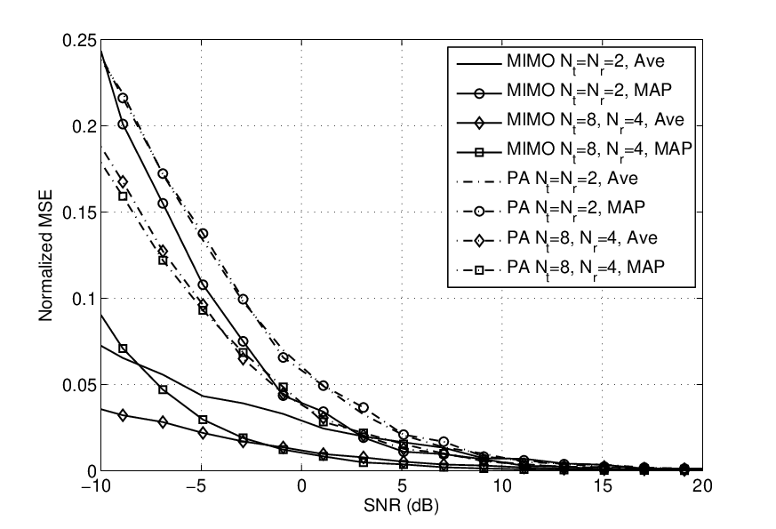
Figure 2: Average normalized MSE of time-delay estimates versus 𝖲𝖭𝖱{\sf SNR} for extended targets.
Refer to caption
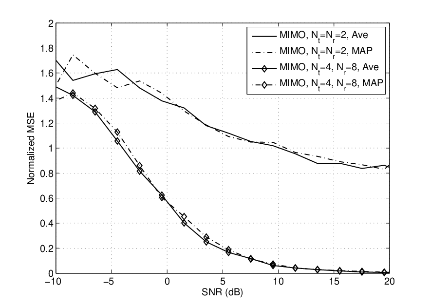
Figure 3: Average normalized MSE of location estimates versus 𝖲𝖭𝖱{\sf SNR} for extended targets.
Refer to caption
Figure 4: Probability of mis-detection versus 𝖲𝖭𝖱{\sf SNR} for a false alarm Pf​a=10−6P_{fa}=10^{-6} for extended targets.
Refer to caption
Figure 5: Probability of target detection versus probability of false alarm for 𝖲𝖭𝖱=0{\sf SNR}=0 dB for extended targets.

We first consider the performance of parameter estimation. Fig. 2 depicts the average normalized mean-square errors (MSE), i.e., 1Nt​Nr​∑m∑n|τ^m,n−τm,nτm,n|2\frac{1}{N_{t}N_{r}}\sum_{m}\sum_{n}\big|\frac{\hat{\tau}_{m,n}-\tau_{m,n}}{\tau_{m,n}}\big|^{2}, for phased-array and MIMO radars as a function of received 𝖲𝖭𝖱{\sf SNR}. It is observed that the MIMO radar outperforms the phased-array in all 𝖲𝖭𝖱{\sf SNR} regimes and in particular, by a large margin in the low 𝖲𝖭𝖱{\sf SNR} regime, which is of more interest in radar applications. Moreover, it is seen that in MIMO radars, the MAP estimator 𝝉^MAP\hat{\boldsymbol{\tau}}^{\rm MAP} performs better than the estimator 𝝉^ave\hat{\boldsymbol{\tau}}^{\textrm{ave}}in the high 𝖲𝖭𝖱{\sf SNR} regime, while the estimator 𝝉^ave\hat{\boldsymbol{\tau}}^{\textrm{ave}} outperforms the MAP estimator 𝝉^MAP\hat{\boldsymbol{\tau}}^{\textrm{MAP}} in the low 𝖲𝖭𝖱{\sf SNR} regime, as expected and discussed in Section 4.1.

It should be noted that comparing the accuracies of the time-delay estimators are not as informative as comparing the accuracies of the detectors. This is mainly because the time-delay estimates have different roles in MIMO and phased-array radars. Nevertheless, we perform such comparisons as the detectors accuracies in our formulations depend on the estimators accuracies, which justifies comparing the time-delay estimator in MIMO and phased-array radars.

We next illustrate the localization performance of MIMO radar in Fig. 3. Once the vector 𝝉^\hat{\boldsymbol{\tau}} is available, it is then possible to further estimate the location X0X_{0} of the gravity center of the target. The localization problem can be formulated in the form of the following nonlinear equations

𝝉^=ϕ⁡(X0)+𝝎,\hat{\boldsymbol{\tau}}=\boldsymbol{\phi}(X_{0})+\boldsymbol{\omega}, (28)

where 𝝎\boldsymbol{\omega} is the noise term, and ϕ⁡(X0)=[ϕ1,1​(X0),…,ϕNt,Nr​(X0)]\boldsymbol{\phi}(X_{0})=\left[\phi_{1,1}(X_{0}),\dots,\phi_{N_{t},N_{r}}(X_{0})\right] is the vector of functions defined as

ϕm,n(X0)=△1c(∥X0−Xmt∥+∥X0−Xnr∥),m=1,…,Nt,n=1,…,Nr,\phi_{m,n}(X_{0})\stackrel{{\scriptstyle\scriptscriptstyle\triangle}}{{=}}\frac{1}{c}\left(\|X_{0}-X_{m}^{t}\|+\|X_{0}-X_{n}^{r}\|\right),m=1,\dots,N_{t},\;n=1,\dots,N_{r}, (29)

where XmtX_{m}^{t} and XnrX_{n}^{r} are the positions of the mt​hm^{th} and nt​hn^{th} transmit and receive antennas respectively. We can solve for X0X_{0} from (28) iteratively as follows. Denote X0(i)X^{(i)}_{0} as the solution at the it​hi^{th} iteration. By linearizing ϕ⁡(X0(i+1))\boldsymbol{\phi}(X^{(i+1)}_{0}) with respect to X0(i)X^{(i)}_{0} we get

ϕ⁡(X0(i+1))≈ϕ⁡(X0(i))+𝑯0​(X0(i))​(X0(i+1)−X0(i)),\boldsymbol{\phi}(X^{(i+1)}_{0})\approx\boldsymbol{\phi}(X^{(i)}_{0})+{\boldsymbol{H}}_{0}(X_{0}^{(i)})\;(X_{0}^{(i+1)}-X_{0}^{(i)}), (30)

where 𝑯0​(X0(i)){\boldsymbol{H}}_{0}(X_{0}^{(i)}) is the Jacobian of the function ϕ(.)\boldsymbol{\phi}(.) evaluated at X0(i)X_{0}^{(i)}. Then, the least-square estimate of the position X0X_{0} based on (28) and (30) is given by

X0(i+1)=arg⁡minX0​[𝒚⁡(X0(i))−𝑯0​(X0(i))​X0]T​[𝒚⁡(X0(i))−𝑯0​(X0(i))​X0],X_{0}^{(i+1)}=\arg\min_{X_{0}}\left[{\boldsymbol{y}}(X_{0}^{(i)})-{\boldsymbol{H}}_{0}(X_{0}^{(i)})\;X_{0}\right]^{T}\left[{\boldsymbol{y}}(X_{0}^{(i)})-{\boldsymbol{H}}_{0}(X_{0}^{(i)})\;X_{0}\right], (31)

where 𝒚⁡(X0(i))=△𝝉−(ϕ⁡(X0(i))−𝑯0​X0(i)){\boldsymbol{y}}(X_{0}^{(i)})\stackrel{{\scriptstyle\scriptscriptstyle\triangle}}{{=}}\boldsymbol{\tau}-\left(\boldsymbol{\phi}(X_{0}^{(i)})-{\boldsymbol{H}}_{0}X_{0}^{(i)}\right) and therefore X0(i+1)X^{(i+1)}_{0} has to satisfy the normal equation

[𝑯0​(X0(i))T​𝑯0​(X0(i))]​X0(i+1)=𝑯0​(X0(i))T​𝒚​(X0(i)).\left[{\boldsymbol{H}}_{0}(X_{0}^{(i)})^{T}{\boldsymbol{H}}_{0}(X_{0}^{(i)})\right]X^{(i+1)}_{0}={\boldsymbol{H}}_{0}(X_{0}^{(i)})^{T}{\boldsymbol{y}}(X_{0}^{(i)}). (32)

An initial estimate X0(0)X_{0}^{(0)} can be obtained, e.g., using the method in [18]. It is seen that the 4×84\times 8 MIMO radar performs considerably better than the 2×22\times 2 MIMO radar, which is due to the fact that 32 time-delays provide much more information about the position of the target than 4 time-delays do.

Finally we consider the detection performance. In Fig. 4 the probability of mis-detection versus 𝖲𝖭𝖱{\sf SNR} is illustrated. The tests are designed such that the probability of false alarm is Pf​a≤10−6P_{fa}\leq 10^{-6}. As analyzed in Section 7 and observed in this figure, the slope of the mis-detection probability of the phased-array radar is 1 decade per 10 dB, whereas that of the MIMO radar is Nt​NrN_{t}N_{r} times steeper. Figure 5 shows the receiver operating curve (ROC) for the MIMO and the phased-array systems, for 𝖲𝖭𝖱=0{\sf SNR}=0 dB. It is seen that the MIMO radar significantly outperforms the phased-array radar over a wide range of false alarm values.

8.2 Point Targets
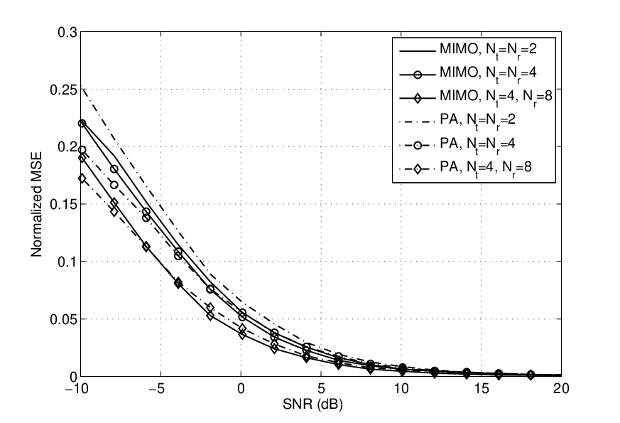
Refer to caption
Figure 6: Average normalized MSE of time-delay estimates versus 𝖲𝖭𝖱{\sf SNR} for point targets.
Refer to caption
Figure 7: Probability of mis-detection versus 𝖲𝖭𝖱{\sf SNR} for point targets and Pf​a=10−6P_{fa}=10^{-6} for point targets.
Refer to caption
Figure 8: Probability of target detection versus probability of false alarm for point targets and 𝖲𝖭𝖱{\sf SNR}=0 dB for point targets.

We use a similar system setup as in Section 8.1. Fig. 6 illustrates the normalized average MSE in estimating the time-delays versus 𝖲𝖭𝖱{\sf SNR}. Unlike for extended targets, it is observed that for point targets, conventional phased-array and MIMO radars exhibit similar target detection and time-delay estimation accuracies. Therefore, when considering joint target detection and time-delay estimation, deploying MIMO radars are not much advantageous for point targets. This conclusion is nevertheless limited to the specific problem analyzed in this paper and MIMO radars can be potentially advantageous in other scenarios like those discussed in [4] and references therein. This is due to the fact that point targets lack independent scattering section and thereof provide no diversity gain.

In Fig. 7 and Fig. 8 the probability of mis-detection versus 𝖲𝖭𝖱{\sf SNR} and the ROC are plotted, respectively. For Fig. 7 the tests are designed such that the probability of false alarm is Pf​a≤10−6P_{fa}\leq 10^{-6} and for Fig. 8 we have set 𝖲𝖭𝖱{\sf SNR}=0 dB. It is seen from Fig. 7 that both the phase-array and the MIMO radars exhibit a diversity gain of 1, which verifies Theorem 4.

9 Conclusions

In this paper we have offered a framework for jointly detecting the presence of a target and estimating some unknown target parameters. We have provided a composite hypothesis test that satisfies some optimality criteria for both target detection and parameter estimation. By using this framework we have proposed a new MIMO radar model for detecting the presence of a target in an unknown location and formulated a composite hypothesis test for solving this problem. In this problem, the unknown parameter of interest to be jointly estimated along with target detection, is the vector of time-delays that a transmitted waveform experiences from being emitted by the transmit antennas until being received by the receive antennas. For the proposed detection scheme, we also have analyzed the decay rate of the probability of mis-detection with increasing 𝖲𝖭𝖱{\sf SNR} while the false-alarm probability is kept below a certain level (diversity gain). Our simulation results demonstrate that for the specific problem of joint target detection and time-delay estimation, deploying MIMO radars is advantageous for extended targets. On the other hand, for point targets, the accuracies of target detection and time-delay estimation by conventional phased-array are comparable with those yielded by MIMO radars.

Appendix A Proof of Theorem 2

The pdf of the vector of received signals 𝑹{\boldsymbol{R}} for any given 𝝉\boldsymbol{\tau} and 𝒉{\boldsymbol{h}} is given by

f1​(𝑹|𝝉,𝒉)\displaystyle f_{1}({\boldsymbol{R}}\;|\;{\boldsymbol{\tau}},{\boldsymbol{h}}) =(π)−K​Nr​exp⁡(−∑n=1Nr∑k=1K|rn​[k]−ENt​c−β​∑m=1Nt1τm,nβ​hm,n​sm​[k;τm,n]|2⏟=△D1​(𝝉,𝒉)).\displaystyle=(\pi)^{-KN_{r}}\exp\Bigg(-\underset{\stackrel{{\scriptstyle\scriptscriptstyle\triangle}}{{=}}D_{1}(\boldsymbol{\tau},{\boldsymbol{h}})}{\underbrace{\sum_{n=1}^{N_{r}}\sum_{k=1}^{K}\left|r_{n}[k]-\sqrt{\frac{E}{N_{t}}}\;c^{-\beta}\;\sum_{m=1}^{N_{t}}\frac{1}{\tau^{\beta}_{m,n}}\;h_{m,n}\;s_{m}[k;\tau_{m,n}]\right|^{2}}}\Bigg). (33)

By taking into account the orthogonality assumption ∑k=1Ksm​[k;τm,n]​sm′∗​[k;τm′,n]=δ⁡(m−m′)Ts\sum_{k=1}^{K}s_{m}[k;\tau_{m,n}]\;s^{*}_{m^{\prime}}[k;\tau_{m^{\prime},n}]=\frac{\delta(m-m^{\prime})}{T_{s}}, we can further simplify the term D1​(𝝉,𝒉)D_{1}(\boldsymbol{\tau},{\boldsymbol{h}}) defined in (33) as follows.

D1​(𝝉,𝒉)\displaystyle D_{1}(\boldsymbol{\tau},{\boldsymbol{h}}) =∑n=1Nr∑k=1K|rn​[k]−ENt​c−β​∑m=1Nt1τm,nβ​hm,n​sm​[k;τm,n]|2\displaystyle=\sum_{n=1}^{N_{r}}\sum_{k=1}^{K}\left|r_{n}[k]-\sqrt{\frac{E}{N_{t}}}\;c^{-\beta}\;\sum_{m=1}^{N_{t}}\frac{1}{\tau^{\beta}_{m,n}}\;h_{m,n}\;s_{m}[k;\tau_{m,n}]\right|^{2}
=∑k=1K‖𝒓⁡[k]‖2+ENt​c−2​β​∑n=1Nr∑m=1Nt∑m′=1Nt1τm,nβ​τm′,nβ​hm,n​hm′,n∗​∑k=1Ksm​[k;τm,n]​sm′∗​[k;τm′,n]⏟1Ts​δ​(m−m′)\displaystyle=\sum_{k=1}^{K}\|{\boldsymbol{r}}[k]\|^{2}+\frac{E}{N_{t}}\;c^{-2\beta}\;\sum_{n=1}^{N_{r}}\ \sum_{m=1}^{N_{t}}\sum_{m^{\prime}=1}^{N_{t}}\frac{1}{\tau^{\beta}_{m,n}\tau^{\beta}_{m^{\prime},n}}\;h_{m,n}\;h^{*}_{m^{\prime},n}\;\underset{\frac{1}{T_{s}}\;\delta(m-m^{\prime})}{\underbrace{\sum_{k=1}^{K}s_{m}[k;\tau_{m,n}]\;s^{*}_{m^{\prime}}[k;\tau_{m^{\prime},n}]}}
−ENtc−β∑n=1Nr∑m=1Nthm,n1τm,nβ∑k=1Krn∗[k]sm[k;τm,n]\displaystyle-\sqrt{\frac{E}{N_{t}}}\;c^{-\beta}\sum_{n=1}^{N_{r}}\sum_{m=1}^{N_{t}}h_{m,n}\;\frac{1}{\tau^{\beta}_{m,n}}\;\sum_{k=1}^{K}r^{*}_{n}[k]\;s_{m}[k;\tau_{m,n}]
−ENtc−β∑n=1Nr∑m=1Nthm,n∗1τm,nβ∑k=1Krn[k]sm∗[k;τm,n]\displaystyle-\sqrt{\frac{E}{N_{t}}}\;c^{-\beta}\sum_{n=1}^{N_{r}}\sum_{m=1}^{N_{t}}h^{*}_{m,n}\;\frac{1}{\tau^{\beta}_{m,n}}\;\sum_{k=1}^{K}r_{n}[k]\;s^{*}_{m}[k;\tau_{m,n}]
=∑k=1K‖𝒓⁡[k]‖2+ETs​Nt​c−2​β​∑n=1Nr∑m=1Nt1τ2​βm,n​|hm,n|2\displaystyle=\sum_{k=1}^{K}\|{\boldsymbol{r}}[k]\|^{2}+\frac{E}{T_{s}N_{t}}\;c^{-2\beta}\sum_{n=1}^{N_{r}}\sum_{m=1}^{N_{t}}\frac{1}{\tau^{2\beta_{m,n}}}\;|h_{m,n}|^{2}
−∑n=1Nr∑m=1Nthm,nENt​c−βτm,nβ​∑k=1Krn∗​[k]​sm​[k;τm,n]⏟=△am,n∗​(τm,n)\displaystyle-\sum_{n=1}^{N_{r}}\sum_{m=1}^{N_{t}}h_{m,n}\;\underset{\stackrel{{\scriptstyle\scriptscriptstyle\triangle}}{{=}}\;a^{*}_{m,n}(\tau_{m,n})}{\underbrace{\sqrt{\frac{E}{N_{t}}}\;\frac{c^{-\beta}}{\tau^{\beta}_{m,n}}\sum_{k=1}^{K}r^{*}_{n}[k]\;s_{m}[k;\tau_{m,n}]}}
−∑n=1Nr∑m=1Nth∗m,nENt​c−βτm,nβ​∑k=1Krn​[k]​sm∗​[k;τm,n]⏟am,n​(τm,n).\displaystyle-\sum_{n=1}^{N_{r}}\sum_{m=1}^{N_{t}}h^{*}_{m,n}\;\underset{a_{m,n}(\tau_{m,n})}{\underbrace{\sqrt{\frac{E}{N_{t}}}\;\frac{c^{-\beta}}{\tau^{\beta}_{m,n}}\sum_{k=1}^{K}r_{n}[k]\;s^{*}_{m}[k;\tau_{m,n}]}}. (34)

For any given time-delay vector 𝝉\boldsymbol{\tau}, define

𝑨𝝉=△ETs​Nt​c−2​β​diag​(τ1,1−2​β,τ1,2−2​β,…,τNt,Nr−2​β)and𝒂𝝉=△[a1,1​(τ1,1),a1,2​(τ1,2),…,aNt,Nr​(τNt,Nr)]T.{\boldsymbol{A}}_{\boldsymbol{\tau}}\stackrel{{\scriptstyle\scriptscriptstyle\triangle}}{{=}}\frac{E}{T_{s}N_{t}}\;c^{-2\beta}\textrm{diag}(\tau^{-2\beta}_{1,1},\tau^{-2\beta}_{1,2},...,\tau^{-2\beta}_{N_{t},N_{r}})\quad{\rm and}\quad{\boldsymbol{a}}_{\boldsymbol{\tau}}\stackrel{{\scriptstyle\scriptscriptstyle\triangle}}{{=}}[a_{1,1}(\tau_{1,1}),a_{1,2}(\tau_{1,2}),\dots,a_{N_{t},N_{r}}(\tau_{N_{t},N_{r}})]^{T}. (35)

Then, D1​(𝝉,𝒉)D_{1}(\boldsymbol{\tau},{\boldsymbol{h}}) can be represented in the matrix form as

D1​(𝝉,𝒉)\displaystyle D_{1}(\boldsymbol{\tau},{\boldsymbol{h}}) =\displaystyle= ∑k=1K‖𝒓⁡[k]‖2+𝒉H​𝑨𝝉​𝒉−𝒉H​𝒂𝝉−𝒂𝝉H​𝒉.\displaystyle\sum_{k=1}^{K}\|{\boldsymbol{r}}[k]\|^{2}+{\boldsymbol{h}}^{H}{\boldsymbol{A}}_{\boldsymbol{\tau}}\;{\boldsymbol{h}}-{\boldsymbol{h}}^{H}{\boldsymbol{a}}_{\boldsymbol{\tau}}-{\boldsymbol{a}}_{\boldsymbol{\tau}}^{H}{\boldsymbol{h}}. (36)

By noting that the pdf of 𝒉{\boldsymbol{h}} is given by f𝒉​(𝒉)=(π)−Nt​Nr​exp⁡(−‖𝒉‖2)f_{\boldsymbol{h}}({\boldsymbol{h}})=(\pi)^{-N_{t}N_{r}}\exp({-\|{\boldsymbol{h}}\|^{2}}), we find the estimates of 𝝉\boldsymbol{\tau} as follows.

  1. 1.

    For finding 𝝉^MAP\hat{\boldsymbol{\tau}}^{\rm MAP} by denoting the MAP estimate of 𝒉{\boldsymbol{h}} by 𝒉^\hat{\boldsymbol{h}}, setting 𝒙=[𝝉^MAP,𝒉^]{\boldsymbol{x}}=[\hat{\boldsymbol{\tau}}^{\rm MAP},\;\hat{\boldsymbol{h}}], and considering the independence of 𝝉\boldsymbol{\tau} and 𝒉{\boldsymbol{h}}, from (11) we get

    [𝝉^MAP;𝒉^]=arg⁡max𝝉∈𝒜⁡(𝒳),𝒉​f1​(𝑹|𝝉,𝒉)​f𝒉​(𝒉)=arg⁡max𝝉∈𝒜⁡(𝒳)⁡arg⁡max𝒉​f1​(𝑹|𝝉,𝒉)​f𝒉​(𝒉),[\hat{\boldsymbol{\tau}}^{\rm MAP};\;\hat{\boldsymbol{h}}]=\arg\max_{\boldsymbol{\tau}\in{\cal A}({\cal X}),{\boldsymbol{h}}}f_{1}({\boldsymbol{R}}\;|\;\boldsymbol{\tau},{\boldsymbol{h}})f_{\boldsymbol{h}}({\boldsymbol{h}})=\arg\max_{\boldsymbol{\tau}\in{\cal A}({\cal X})}\arg\max_{{\boldsymbol{h}}}f_{1}({\boldsymbol{R}}\;|\;\boldsymbol{\tau},{\boldsymbol{h}})f_{\boldsymbol{h}}({\boldsymbol{h}}),

    or equivalently

    𝒉^=arg⁡max𝒉​f1​(𝑹|𝝉,𝒉)​f𝒉​(𝒉),and𝝉^MAP=arg⁡max𝝉∈𝒜⁡(𝒳)​f1​(𝑹|𝝉,𝒉^)​f𝒉​(𝒉^).\hat{\boldsymbol{h}}=\arg\max_{{\boldsymbol{h}}}f_{1}({\boldsymbol{R}}\;|\;\boldsymbol{\tau},{\boldsymbol{h}})f_{\boldsymbol{h}}({\boldsymbol{h}}),\quad\mbox{and}\quad\hat{\boldsymbol{\tau}}^{\rm MAP}=\arg\max_{\boldsymbol{\tau}\in{\cal A}({\cal X})}f_{1}({\boldsymbol{R}}\;|\;\boldsymbol{\tau},\hat{\boldsymbol{h}})f_{\boldsymbol{h}}(\hat{\boldsymbol{h}}). (37)

    Using (33), (36), and (37) and noting the definition of 𝒂𝝉{\boldsymbol{a}}_{\boldsymbol{\tau}} given in (35) provides that

    𝒉^\displaystyle\hat{\boldsymbol{h}} =\displaystyle= arg⁡max𝒉​f1​(𝑹|𝝉,𝒉)​f𝒉​(𝒉)\displaystyle\arg\max_{{\boldsymbol{h}}}f_{1}({\boldsymbol{R}}\;|\;\boldsymbol{\tau},{\boldsymbol{h}})f_{\boldsymbol{h}}({\boldsymbol{h}}) (38)
    =\displaystyle= arg⁡max𝒉​(π)−Nt​Nr+K​Nr​exp⁡(−(∑k‖𝒓⁡[k]‖2+𝒉H​𝑨𝝉​𝒉−𝒉H​𝒂𝝉−𝒂𝝉H​𝒉+‖𝒉‖2))\displaystyle\arg\max_{{\boldsymbol{h}}}(\pi)^{-N_{t}N_{r}+KN_{r}}\exp\left(-\left(\sum_{k}\|{\boldsymbol{r}}[k]\|^{2}+{\boldsymbol{h}}^{H}{\boldsymbol{A}}_{\boldsymbol{\tau}}{\boldsymbol{h}}-{\boldsymbol{h}}^{H}{\boldsymbol{a}}_{\boldsymbol{\tau}}-{\boldsymbol{a}}_{\boldsymbol{\tau}}^{H}{\boldsymbol{h}}+\|{\boldsymbol{h}}\|^{2}\right)\right)
    =\displaystyle= arg⁡min𝒉​{𝒉H​(𝑨𝝉+𝑰Nt​Nr)⏟=△𝑩𝝉​𝒉−𝒉H​𝒂𝝉−𝒂𝝉H​𝒉}\displaystyle\arg\min_{{\boldsymbol{h}}}\bigg\{{\boldsymbol{h}}^{H}\underset{\stackrel{{\scriptstyle\scriptscriptstyle\triangle}}{{=}}{\boldsymbol{B}}_{\boldsymbol{\tau}}}{\underbrace{\left({\boldsymbol{A}}_{\boldsymbol{\tau}}+{\boldsymbol{I}}_{N_{t}N_{r}}\right)}}{\boldsymbol{h}}-{\boldsymbol{h}}^{H}{\boldsymbol{a}}_{\boldsymbol{\tau}}-{\boldsymbol{a}}_{\boldsymbol{\tau}}^{H}{\boldsymbol{h}}\bigg\}
    =\displaystyle= 𝑩𝝉−1​𝒂𝝉.\displaystyle{\boldsymbol{B}}_{\boldsymbol{\tau}}^{-1}{\boldsymbol{a}}_{\boldsymbol{\tau}}.

    Based on the above estimate of 𝝉\boldsymbol{\tau}, D1​(𝝉,𝒉^)D_{1}(\boldsymbol{\tau},\hat{\boldsymbol{h}}) given in (36) becomes

    D1​(𝝉,𝒉^)\displaystyle D_{1}(\boldsymbol{\tau},\hat{\boldsymbol{h}}) =\displaystyle= ∑k=1K‖𝒓⁡[k]‖2−𝒂𝝉H​𝑩−1​𝒂𝝉−‖𝒉^‖2.\displaystyle\sum_{k=1}^{K}\|{\boldsymbol{r}}[k]\|^{2}-{\boldsymbol{a}}_{\boldsymbol{\tau}}^{H}{\boldsymbol{B}}^{-1}{\boldsymbol{a}}_{\boldsymbol{\tau}}-\|\hat{\boldsymbol{h}}\|^{2}. (39)

    Hence, the ML estimate of 𝝉\boldsymbol{\tau} can be found by solving

    𝝉^MAP=arg⁡max𝝉∈𝒜⁡(𝒳)⁡log⁡f1​(𝑹|𝝉,𝒉^)​f𝒉​(𝒉^)\displaystyle\hat{\boldsymbol{\tau}}^{\rm MAP}=\arg\max_{\boldsymbol{\tau}\in{\cal A}({\cal X})}\log f_{1}({\boldsymbol{R}}\;|\;\boldsymbol{\tau},\hat{\boldsymbol{h}})f_{{\boldsymbol{h}}}(\hat{\boldsymbol{h}}) =arg⁡max𝝉∈𝒜⁡(𝒳)​{−D1​(𝝉,𝒉^)−‖𝒉^‖2}\displaystyle=\arg\max_{\boldsymbol{\tau}\in{\cal A}({\cal X})}\left\{-D_{1}(\boldsymbol{\tau},\hat{\boldsymbol{h}})-\|\hat{\boldsymbol{h}}\|^{2}\right\}
    =arg⁡max𝝉∈𝒜⁡(𝒳)​{𝒂𝝉H​𝑩𝝉−1​𝒂𝝉}\displaystyle=\arg\max_{\boldsymbol{\tau}\in{\cal A}({\cal X})}\left\{{\boldsymbol{a}}_{\boldsymbol{\tau}}^{H}{\boldsymbol{B}}^{-1}_{\boldsymbol{\tau}}{\boldsymbol{a}}_{\boldsymbol{\tau}}\right\} (40)
    =arg⁡max𝝉∈𝒜⁡(𝒳)​{𝒂𝝉H​(𝑨𝝉+𝑰)−1​𝒂𝝉}\displaystyle=\arg\max_{\boldsymbol{\tau}\in{\cal A}({\cal X})}\left\{{\boldsymbol{a}}_{\boldsymbol{\tau}}^{H}({\boldsymbol{A}}_{\boldsymbol{\tau}}+{\boldsymbol{I}})^{-1}{\boldsymbol{a}}_{\boldsymbol{\tau}}\right\}
    =arg⁡max𝝉∈𝒜⁡(𝒳)​{∑m=1Nt∑n=1Nr|am,n​(τm,n)|2ETs​Nt​(c​τm,n)−2​β+1},\displaystyle=\arg\max_{\boldsymbol{\tau}\in{\cal A}({\cal X})}\left\{\sum_{m=1}^{N_{t}}\sum_{n=1}^{N_{r}}\frac{|a_{m,n}(\tau_{m,n})|^{2}}{\frac{E}{T_{s}N_{t}}(c\tau_{m,n})^{-2\beta}+1}\right\}, (41)

    which concludes the proof.

  2. 2.

    For this case which we average out the effect of 𝒉{\boldsymbol{h}} by setting 𝒙=𝝉{\boldsymbol{x}}=\boldsymbol{\tau} from (11) we get

    𝝉^ave\displaystyle\hat{\boldsymbol{\tau}}^{\rm ave} =\displaystyle= arg⁡max𝝉∈𝒜⁡(𝒳)​f1​(𝑹|𝝉)=arg⁡max⁡∫𝒉𝝉∈𝒜⁡(𝒳)⁡f1​(𝑹|τ,𝒉)​f𝒉​(𝒉)​𝑑𝒉\displaystyle\arg\max_{\boldsymbol{\tau}\in{\cal A}({\cal X})}f_{1}({\boldsymbol{R}}\;|\;{\boldsymbol{\tau}})=\arg\max_{\boldsymbol{\tau}\in{\cal A}({\cal X})}\int_{\boldsymbol{h}}f_{1}({\boldsymbol{R}}\;|\;{\mathbb{\tau}},{\boldsymbol{h}})f_{\boldsymbol{h}}({\boldsymbol{h}})\;d{\boldsymbol{h}} (42)
    =\displaystyle= arg⁡max⁡∫𝒉𝝉∈𝒜⁡(𝒳)⁡exp⁡(−D1​(𝝉,𝒉))​f𝒉​(𝒉)​𝑑𝒉\displaystyle\arg\max_{\boldsymbol{\tau}\in{\cal A}({\cal X})}\int_{\boldsymbol{h}}\exp\Big(-D_{1}(\boldsymbol{\tau},{\boldsymbol{h}})\Big)f_{\boldsymbol{h}}({\boldsymbol{h}})\;d{\boldsymbol{h}}
    =\displaystyle= arg⁡max⁡∫𝒉𝝉∈𝒜⁡(𝒳)⁡exp⁡(−(𝒉H​(𝑨𝝉+𝑰Nt​Nr)⏟=△𝑩𝝉​𝒉−𝒉H​𝒂𝝉−𝒂𝝉H​𝒉))​𝑑𝒉\displaystyle\arg\max_{\boldsymbol{\tau}\in{\cal A}({\cal X})}\int_{\boldsymbol{h}}\exp\bigg(-\Big({\boldsymbol{h}}^{H}\underset{\stackrel{{\scriptstyle\scriptscriptstyle\triangle}}{{=}}{\boldsymbol{B}}_{\boldsymbol{\tau}}}{\underbrace{\left({\boldsymbol{A}}_{\boldsymbol{\tau}}+{\boldsymbol{I}}_{N_{t}N_{r}}\right)}}{\boldsymbol{h}}-{\boldsymbol{h}}^{H}{\boldsymbol{a}}_{\boldsymbol{\tau}}-{\boldsymbol{a}}_{\boldsymbol{\tau}}^{H}{\boldsymbol{h}}\Big)\bigg)\;d{\boldsymbol{h}}
    =\displaystyle= arg⁡max⁡∫𝒉𝝉∈𝒜⁡(𝒳)⁡exp⁡(−{(𝒉−𝑩𝝉−1​𝒂𝝉)H​𝑩𝝉​(𝒉−𝑩𝝉−1​𝒂𝝉)−𝒂𝝉H​𝑩𝝉−1​𝒂𝝉})​𝑑𝒉\displaystyle\arg\max_{\boldsymbol{\tau}\in{\cal A}({\cal X})}\int_{\boldsymbol{h}}\exp\left({-\left\{\left({\boldsymbol{h}}-{\boldsymbol{B}}_{\boldsymbol{\tau}}^{-1}{\boldsymbol{a}}_{\boldsymbol{\tau}}\right)^{H}{\boldsymbol{B}}_{\boldsymbol{\tau}}\;\left({\boldsymbol{h}}-{\boldsymbol{B}}_{\boldsymbol{\tau}}^{-1}{\boldsymbol{a}}_{\boldsymbol{\tau}}\right)-{\boldsymbol{a}}_{\boldsymbol{\tau}}^{H}{\boldsymbol{B}}_{\boldsymbol{\tau}}^{-1}{\boldsymbol{a}}_{\boldsymbol{\tau}}\right\}}\right)\;d{\boldsymbol{h}} (43)
    =\displaystyle= arg⁡max𝝉∈𝒜⁡(𝒳)​exp⁡(𝒂𝝉H​𝑩𝝉−1​𝒂𝝉)​∫𝒉exp⁡(−{(𝒉−𝑩𝝉−1​𝒂𝝉)H​𝑩𝝉​(𝒉−𝑩𝝉−1​𝒂𝝉)})​𝑑𝒉\displaystyle\arg\max_{\boldsymbol{\tau}\in{\cal A}({\cal X})}\exp\left({\boldsymbol{a}}_{\boldsymbol{\tau}}^{H}{\boldsymbol{B}}_{\boldsymbol{\tau}}^{-1}{\boldsymbol{a}}_{\boldsymbol{\tau}}\right)\int_{\boldsymbol{h}}\exp\left({-\left\{\left({\boldsymbol{h}}-{\boldsymbol{B}}_{\boldsymbol{\tau}}^{-1}{\boldsymbol{a}}_{\boldsymbol{\tau}}\right)^{H}{\boldsymbol{B}}_{\boldsymbol{\tau}}\;\left({\boldsymbol{h}}-{\boldsymbol{B}}_{\boldsymbol{\tau}}^{-1}{\boldsymbol{a}}_{\boldsymbol{\tau}}\right)\right\}}\right)\;d{\boldsymbol{h}}
    =\displaystyle= arg⁡max𝝉∈𝒜​exp⁡(𝒂𝝉H​𝑩𝝉−1​𝒂𝝉)​|𝑩𝝉|−1\displaystyle\arg\max_{\boldsymbol{\tau}\in{\cal A}}\exp\left({\boldsymbol{a}}_{\boldsymbol{\tau}}^{H}{\boldsymbol{B}}_{\boldsymbol{\tau}}^{-1}{\boldsymbol{a}}_{\boldsymbol{\tau}}\right)\;|{\boldsymbol{B}}_{\boldsymbol{\tau}}|^{-1} (44)
    =\displaystyle= arg⁡max𝝉∈𝒜⁡(𝒳)​{𝒂𝝉H​𝑩𝝉−1​𝒂𝝉−log⁡|𝑩𝝉|}\displaystyle\arg\max_{\boldsymbol{\tau}\in{\cal A}({\cal X})}\left\{{\boldsymbol{a}}_{\boldsymbol{\tau}}^{H}{\boldsymbol{B}}_{\boldsymbol{\tau}}^{-1}{\boldsymbol{a}}_{\boldsymbol{\tau}}-\log|{\boldsymbol{B}}_{\boldsymbol{\tau}}|\right\}
    =\displaystyle= arg⁡max𝝉∈𝒜⁡(𝒳)​{𝒂𝝉H​(𝑨𝝉+𝑰)−1​𝒂𝝉−log⁡|𝑨𝝉+𝑰|}\displaystyle\arg\max_{\boldsymbol{\tau}\in{\cal A}({\cal X})}\left\{{\boldsymbol{a}}_{\boldsymbol{\tau}}^{H}({\boldsymbol{A}}_{\boldsymbol{\tau}}+{\boldsymbol{I}})^{-1}{\boldsymbol{a}}_{\boldsymbol{\tau}}-\log|{\boldsymbol{A}}_{\boldsymbol{\tau}}+{\boldsymbol{I}}|\right\}
    =\displaystyle= arg⁡max𝝉∈𝒜⁡(𝒳)​∑m=1Nt∑n=1Nr{|am,n​(τm,n)|2ETs​Nt​(c​τm,n)−2​β+1−log⁡(ETs​Nt​(c​τm,n)−2​β+1)}.\displaystyle\arg\max_{\boldsymbol{\tau}\in{\cal A}({\cal X})}\sum_{m=1}^{N_{t}}\sum_{n=1}^{N_{r}}\left\{\frac{|a_{m,n}(\tau_{m,n})|^{2}}{\frac{E}{T_{s}N_{t}}(c\tau_{m,n})^{-2\beta}+1}-\log\left(\frac{E}{T_{s}N_{t}}(c\tau_{m,n})^{-2\beta}+1\right)\right\}.

    Noting the definition of am,n​(τm,n)a_{m,n}(\tau_{m,n}) given in (34) concludes the proof.

Appendix B Proof of Theorem 3

In order to find the ML estimate of 𝝉\boldsymbol{\tau} and ζ\zeta form (11) we have

[𝝉,ζ]=arg⁡max𝝉∈𝒜⁡(𝒳),ζ​f1​(𝑹|𝝉,ζ)=arg⁡max𝝉∈𝒜⁡(𝒳)⁡arg⁡maxζ​f1​(𝑹|𝝉,ζ),[\boldsymbol{\tau},\;\zeta]=\arg\max_{\boldsymbol{\tau}\in{\cal A}({\cal X}),\zeta}f_{1}({\boldsymbol{R}}\;|\;\boldsymbol{\tau},\zeta)=\arg\max_{\boldsymbol{\tau}\in{\cal A}({\cal X})}\arg\max_{\zeta}f_{1}({\boldsymbol{R}}\;|\;\boldsymbol{\tau},\zeta),

or equivalently

ζ^=arg⁡maxζ​f1​(𝑹|𝝉,ζ)and𝝉^=arg⁡max𝝉∈𝒜⁡(𝒳)​f1​(𝑹|𝝉,τ^).\hat{\zeta}=\arg\max_{\zeta}f_{1}({\boldsymbol{R}}\;|\;\boldsymbol{\tau},\zeta)\quad\mbox{and}\quad\hat{\boldsymbol{\tau}}=\arg\max_{\boldsymbol{\tau}\in{\cal A}({\cal X})}f_{1}({\boldsymbol{R}}\;|\;\boldsymbol{\tau},\hat{\tau}).

On the other hand, from (5) the likelihood f1​(𝑹|𝝉,τ^)f_{1}({\boldsymbol{R}}\;|\;\boldsymbol{\tau},\hat{\tau}) is given by

f1​(𝑹|𝝉,ζ)=(π)−K​Nr​exp⁡(−∑n=1Nr∑k=1K|rn​[k]−ENt​ζ​c−β​∑m=1Nte−j​2​π​fc​τm,nτm,nβ​sm​[k;τm,n]|2⏟=△D2​(𝝉,ζ)).\displaystyle f_{1}({\boldsymbol{R}}\;|\;\boldsymbol{\tau},\zeta)=(\pi)^{-KN_{r}}\exp\Bigg(-\underset{\stackrel{{\scriptstyle\scriptscriptstyle\triangle}}{{=}}D_{2}(\boldsymbol{\tau},\zeta)}{\underbrace{\sum_{n=1}^{N_{r}}\sum_{k=1}^{K}\bigg|r_{n}[k]-\sqrt{\frac{E}{N_{t}}}\;\zeta\;c^{-\beta}\sum_{m=1}^{N_{t}}\frac{e^{-j2\pi f_{c}\tau_{m,n}}}{\tau^{\beta}_{m,n}}\;s_{m}[k;\tau_{m,n}]\bigg|^{2}}}\Bigg). (45)

By taking into account the orthonormality assumption on sm​[k;τm,n]s_{m}[k;\tau_{m,n}] we get

D2​(𝝉,ζ)\displaystyle D_{2}(\boldsymbol{\tau},\zeta) =\displaystyle= ∑n=1Nr∑k=1K|rn​[k]−ENt​ζ​c−β​∑m=1Nte−j​2​π​fc​τm,nτm,nβ​sm​[k;τm,n]|2\displaystyle\sum_{n=1}^{N_{r}}\sum_{k=1}^{K}\bigg|r_{n}[k]-\sqrt{\frac{E}{N_{t}}}\;\zeta\;c^{-\beta}\sum_{m=1}^{N_{t}}\frac{e^{-j2\pi f_{c}\tau_{m,n}}}{\tau^{\beta}_{m,n}}\;s_{m}[k;\tau_{m,n}]\bigg|^{2} (46)
=\displaystyle= ∑k=1K‖𝒓⁡[k]‖2+ETs​Nt​|ζ|2​c−2​β​∑n=1Nr∑m=1Nt1(c​τm,n)2​β\displaystyle\sum_{k=1}^{K}\|{\boldsymbol{r}}[k]\|^{2}+\frac{E}{T_{s}N_{t}}\left|\zeta\right|^{2}c^{-2\beta}\;\sum_{n=1}^{N_{r}}\sum_{m=1}^{N_{t}}\frac{1}{(c\tau_{m,n})^{2\beta}}
−\displaystyle- ∑n=1Nr∑m=1Nte−j​2​π​fc​τm,n​ENt​ζ​c−βτm,nβ​∑k=1Krn∗​[k]​sm​[k;τm,n]\displaystyle\sum_{n=1}^{N_{r}}\sum_{m=1}^{N_{t}}e^{-j2\pi f_{c}\tau_{m,n}}\;{{\sqrt{\frac{E}{N_{t}}}\;\zeta\;\frac{c^{-\beta}}{\tau^{\beta}_{m,n}}\;\sum_{k=1}^{K}r^{*}_{n}[k]\;s_{m}[k;\tau_{m,n}]}}
−\displaystyle- ∑n=1Nr∑m=1Ntej​2​π​fc​τm,n​ENt​ζ∗​c−βτm,nβ​∑k=1Krn​[k]​sm∗​[k;τm,n].\displaystyle\sum_{n=1}^{N_{r}}\sum_{m=1}^{N_{t}}e^{j2\pi f_{c}\tau_{m,n}}\;{{\sqrt{\frac{E}{N_{t}}}\;\zeta^{*}\;\frac{c^{-\beta}}{\tau^{\beta}_{m,n}}\;\sum_{k=1}^{K}r_{n}[k]\;s^{*}_{m}[k;\tau_{m,n}]}}.

D2​(𝝉,ζ)D_{2}(\boldsymbol{\tau},\zeta) is quadratic in ζ\zeta and its minimum which is attained at the ML estimate of ζ\zeta is given by

ζ^=arg⁡maxζ​log​f1​(𝑹|𝝉,ζ)\displaystyle\hat{\zeta}=\arg\max_{\zeta}\log f_{1}({\boldsymbol{R}}\;|\;{\boldsymbol{\tau}},\zeta) =arg⁡minζ​D2​(𝝉,ζ)\displaystyle=\arg\min_{\zeta}\;D_{2}(\boldsymbol{\tau},\zeta)
=∑m=1Nt∑n=1Nr1(c​τm,n)β​ej​2​π​fc​τm,n​∑k=1Krn​[k]​sm∗​[k;τm,n]1Ts​ENT​∑m=1Nt∑n=1Nr1(c​τm,n)2​β.\displaystyle=\frac{\sum_{m=1}^{N_{t}}\sum_{n=1}^{N_{r}}\;\frac{1}{(c\tau_{m,n})^{\beta}}\;e^{j2\pi f_{c}\tau_{m,n}}\;\sum_{k=1}^{K}r_{n}[k]\;s^{*}_{m}[k;\tau_{m,n}]}{\frac{1}{T_{s}}\sqrt{\frac{E}{N_{T}}}\sum_{m=1}^{N_{t}}\sum_{n=1}^{N_{r}}\;\frac{1}{(c\tau_{m,n})^{2\beta}}}. (47)

By substituting (47) back in (46), and after some manipulation, D2​(𝝉,ζ^)D_{2}(\boldsymbol{\tau},\hat{\zeta}) becomes

D2​(𝝉,ζ^)\displaystyle D_{2}(\boldsymbol{\tau},\hat{\zeta}) =\displaystyle= ∑k=1K‖𝒓⁡[k]‖2−ETs​Nt​|ζ^|2​∑m=1Nt∑n=1Nr1(c​τm,n)2​β.\displaystyle\sum_{k=1}^{K}\|{\boldsymbol{r}}[k]\|^{2}-\frac{E}{T_{s}N_{t}}|\hat{\zeta}\;|^{2}\;\sum_{m=1}^{N_{t}}\sum_{n=1}^{N_{r}}\;\frac{1}{(c\tau_{m,n})^{2\beta}}.

Therefore,

𝝉^=arg⁡max𝝉∈𝒜⁡(𝒳)​log​f1​(𝑹|𝝉,ζ^)\displaystyle\hat{\boldsymbol{\tau}}=\arg\max_{\boldsymbol{\tau}\in{\cal A}({\cal X})}\log f_{1}({\boldsymbol{R}}\;|\;{\boldsymbol{\tau}},\hat{\zeta}) =arg⁡minζ​D2​(𝝉,ζ^)=arg⁡max𝝉∈𝒜⁡(𝒳)​{|ζ^|2​∑m=1Nt∑n=1Nr1(c​τm,n)2​β}\displaystyle=\arg\min_{\zeta}\;D_{2}(\boldsymbol{\tau},\hat{\zeta})=\arg\max_{\boldsymbol{\tau}\in{\cal A}({\cal X})}\Big\{|\hat{\zeta}\;|^{2}\;\sum_{m=1}^{N_{t}}\sum_{n=1}^{N_{r}}\;\frac{1}{(c\tau_{m,n})^{2\beta}}\Big\}
=arg⁡max𝝉∈𝒜⁡(𝒳)⁡|∑m=1Nt∑n=1Nrej​2​π​fc​τm,nτm,nβ​∑k=1Krn​[k]​sm∗​[k;τm,n]|2∑m=1Nt∑n=1Nr1τm,n2​β.\displaystyle=\arg\max_{\boldsymbol{\tau}\in{\cal A}({\cal X})}\frac{\left|\sum_{m=1}^{N_{t}}\sum_{n=1}^{N_{r}}\;\frac{e^{j2\pi f_{c}\tau_{m,n}}}{\tau^{\beta}_{m,n}}\;\sum_{k=1}^{K}r_{n}[k]\;s^{*}_{m}[k;\tau_{m,n}]\right|^{2}}{\sum_{m=1}^{N_{t}}\sum_{n=1}^{N_{r}}\;\frac{1}{\tau^{2\beta}_{m,n}}}. (48)

Appendix C Proof of Lemma 3

We provide the proof by induction.

  1. 1.

    N=2N=2. We define

    q⁡(t1,t2)=△|ej​α​t1​g1​(t1)+ej​α​t2​g2​(t1)|.\displaystyle q(t_{1},t_{2})\stackrel{{\scriptstyle\scriptscriptstyle\triangle}}{{=}}\left|e^{j\alpha t_{1}}g_{1}(t_{1})+e^{j\alpha t_{2}}g_{2}(t_{1})\right|.

    Then

    q2​(t1,t2)=|g1​(t1)|2+|g2​(t1)|2+ej​α​(t1−t2)​g1​(t1)​g2∗​(t1)+ej​α​(t2−t1)​g2​(t1)​g1∗​(t1),\displaystyle q^{2}(t_{1},t_{2})=\left|g_{1}(t_{1})\right|^{2}+\left|g_{2}(t_{1})\right|^{2}+e^{j\alpha(t_{1}-t_{2})}g_{1}(t_{1})g_{2}^{*}(t_{1})+e^{j\alpha(t_{2}-t_{1})}g_{2}(t_{1})g_{1}^{*}(t_{1}),

    and therefore,

    ∂(q2​(t1,t2))∂t2=j​α​[ej​α​(t2−t1)​g2​(t1)​g1∗​(t1)−ej​α​(t1−t2)​g1​(t1)​f2∗​(t1)].\displaystyle\frac{\partial(q^{2}(t_{1},t_{2}))}{\partial t_{2}}=j\alpha\left[e^{j\alpha(t_{2}-t_{1})}g_{2}(t_{1})g_{1}^{*}(t_{1})-e^{j\alpha(t_{1}-t_{2})}g_{1}(t_{1})f^{*}_{2}(t_{1})\right].

    For finding maxt2⁡q⁡(t1,t2)\max_{t_{2}}q(t_{1},t_{2}) we set ∂(q2​(t1,t2))∂t2=0\frac{\partial(q^{2}(t_{1},t_{2}))}{\partial t_{2}}=0 and obtain

    ej​α​t^2=ej​α​t1​g1​(t1)​g2∗​(t1)g1∗​(t1)​g2​(t1).e^{j\alpha\hat{t}_{2}}=e^{j\alpha{t}_{1}}\sqrt{\frac{g_{1}(t_{1})g^{*}_{2}(t_{1})}{g^{*}_{1}(t_{1})g_{2}(t_{1})}}.

    We can check that this is a maximum by noting that

    ∂2(q2​(t1,t2))∂t22|t2=t^2\displaystyle\left.\frac{\partial^{2}(q^{2}(t_{1},t_{2}))}{\partial t_{2}^{2}}\right|_{t_{2}=\hat{t}_{2}} =\displaystyle= (j​α)2​[ej​α​(t^2−t1)​g1∗​(t1)​g2​(t1)+ej​α​(t1−t^2)​g1​(t1)​g2∗​(t1)]\displaystyle(j\alpha)^{2}\left[e^{j\alpha(\hat{t}_{2}-t_{1})}g^{*}_{1}(t_{1})g_{2}(t_{1})+e^{j\alpha(t_{1}-\hat{t}_{2})}g_{1}(t_{1})g^{*}_{2}(t_{1})\right]
    =\displaystyle= −2​(α)2​|g1​(t1)​g2​(t1)|<0,\displaystyle-2(\alpha)^{2}\left|g_{1}(t_{1})g_{2}(t_{1})\right|<0,

    Hence,

    maxt2⁡q⁡(t1,t2)=q⁡(t1,t^2)=|g1​(t1)|2+|g2​(t1)|2+2​|g1​(t1)​g2​(t1)|=∑i=12|gi​(t1)|.\max_{t_{2}}q(t_{1},t_{2})=q(t_{1},\hat{t}_{2})=\sqrt{|g_{1}(t_{1})|^{2}+|g_{2}(t_{1})|^{2}+2|g_{1}(t_{1})g_{2}(t_{1})|}=\sum_{i=1}^{2}|g_{i}(t_{1})|.
  2. 2.

    Inductive assumption.

    max{t2,…,tN}⁡|∑i=1Nej​α​ti​gi​(t1)|=∑i=1N|gi​(t1)|.\max_{\{t_{2},\dots,t_{N}\}}\left|\sum_{i=1}^{N}e^{j\alpha t_{i}}g_{i}(t_{1})\right|=\sum_{i=1}^{N}\left|g_{i}(t_{1})\right|.
  3. 3.

    Claim

    max{t2,…,tN+1}⁡|∑i=1N+1ej​α​ti​gi​(t1)|=∑i=1N+1|gi​(t1)|.\max_{\{t_{2},\dots,t_{N+1}\}}\left|\sum_{i=1}^{N+1}e^{j\alpha t_{i}}g_{i}(t_{1})\right|=\sum_{i=1}^{N+1}\left|g_{i}(t_{1})\right|.

    Let 𝒕=△[t1​…​tN+1]{{\boldsymbol{t}}}\stackrel{{\scriptstyle\scriptscriptstyle\triangle}}{{=}}\left[t_{1}\;\ldots t_{N+1}\right] and q⁡(𝒕)=△|∑i=1N+1ej​α​ti​gi​(t1)|q({{\boldsymbol{t}}})\stackrel{{\scriptstyle\scriptscriptstyle\triangle}}{{=}}\left|\sum_{i=1}^{N+1}e^{j\alpha t_{i}}g_{i}(t_{1})\right|, then

    ∂(q2​(𝒕))∂tN+1\displaystyle\frac{\partial(q^{2}({\boldsymbol{t}}))}{\partial t_{N+1}} =\displaystyle= ∂∂tN+1​[∑i=1Nej​α​(tN+1−ti)​gi∗​(t1)​gN+1​(t1)+∑i=1Nej​α​(ti−tN+1)​gi​(t1)​gN+1∗​(t1)]\displaystyle\frac{\partial}{\partial t_{N+1}}\left[\sum_{i=1}^{N}e^{j\alpha(t_{N+1}-t_{i})}g_{i}^{*}(t_{1})g_{N+1}(t_{1})+\sum_{i=1}^{N}e^{j\alpha(t_{i}-t_{N+1})}g_{i}(t_{1})g^{*}_{N+1}(t_{1})\right]
    =\displaystyle= j​α​[∑i=1Nej​α​(tn+1−ti)​gi∗​(t1)​gN+1​(t1)+∑i=1Nej​α​(ti−tN+1)​gi​(t1)​gN+1∗​(t1)].\displaystyle j\alpha\;\left[\sum_{i=1}^{N}e^{j\alpha(t_{n+1}-t_{i})}g_{i}^{*}(t_{1})g_{N+1}(t_{1})+\sum_{i=1}^{N}e^{j\alpha(t_{i}-t_{N+1})}g_{i}(t_{1})g^{*}_{N+1}(t_{1})\right].

    If we set ∂(q2​(𝒕))∂tn+1=0\frac{\partial(q^{2}({\boldsymbol{t}}))}{\partial t_{n+1}}=0, then

    e2​j​α​t^N+1=∑i=1Nej​α​ti​gi​(t1)∑i=1Ne−j​α​ti​gi∗​(t1)​gN+1∗​(t1)gN+1​(t1).\displaystyle e^{2j\alpha\hat{t}_{N+1}}=\frac{\sum_{i=1}^{N}e^{j\alpha t_{i}}g_{i}(t_{1})}{\sum_{i=1}^{N}e^{-j\alpha t_{i}}g^{*}_{i}(t_{1})}\frac{g^{*}_{N+1}(t_{1})}{g_{N+1}(t_{1})}.

    Also t^N+1\hat{t}_{N+1} is a maximum since

    ∂2(q2​(𝒕))∂tN+12|tN+1=t^N+1\displaystyle\left.\frac{\partial^{2}(q^{2}({\boldsymbol{t}}))}{\partial t_{N+1}^{2}}\right|_{t_{N+1}=\hat{t}_{N+1}} =\displaystyle= (j​α)2​[∑i=1Nej​α​(t^N+1−ti)​gi∗​(t1)​gN+1​(t1)+∑i=1Nej​α​(ti−t^N+1)​gi​(t1)​gN+1∗​(t1)]\displaystyle(j\alpha)^{2}\left[\sum_{i=1}^{N}e^{j\alpha(\hat{t}_{N+1}-t_{i})}g^{*}_{i}(t_{1})g_{N+1}(t_{1})+\sum_{i=1}^{N}e^{j\alpha(t_{i}-\hat{t}_{N+1})}g_{i}(t_{1})g^{*}_{N+1}(t_{1})\right]
    =\displaystyle= (j​α)2​[2​(∑i=1Nej​α​ti​gi​(t1)​gN+1∗​(t1)​∑k=1Ne−j​α​tk​gk∗​(t1)​gN+1​(t1))12]\displaystyle(j\alpha)^{2}\left[2\left(\sum_{i=1}^{N}e^{j\alpha t_{i}}g_{i}(t_{1})g^{*}_{N+1}(t_{1})\sum_{k=1}^{N}e^{-j\alpha t_{k}}g^{*}_{k}(t_{1})g_{N+1}(t_{1})\right)^{\frac{1}{2}}\right]
    =\displaystyle= −2​α2​|∑i=1Nej​α​ti​gi​(t1)​gN+1∗​(t1)|<0.\displaystyle-2\alpha^{2}\left|\sum_{i=1}^{N}e^{j\alpha t_{i}}g_{i}(t_{1})g^{*}_{N+1}(t_{1})\right|<0.

    Therefore by substituting t^N+1\hat{t}_{N+1} and some simple manipulations we get

    maxtN+1⁡q2​(𝒕)=q2​(t1,…,tN,t^N+1)\displaystyle\max_{t_{N+1}}q^{2}({\boldsymbol{t}})=q^{2}(t_{1},...,t_{N},\hat{t}_{N+1}) =|∑i=1Nej​α​ti​gi​(t1)|2+|gN+1​(t1)|2\displaystyle=\left|\sum_{i=1}^{N}e^{j\alpha t_{i}}g_{i}(t_{1})\right|^{2}+\left|g_{N+1}(t_{1})\right|^{2}
    +2​(∑i=1Nej​α​ti​gi​(t1)​gN+1∗​(t1)​∑k=1Ne−j​α​tk​gk∗​(t1)​gN+1​(t1))12\displaystyle+2\left(\sum_{i=1}^{N}e^{j\alpha t_{i}}g_{i}(t_{1})g^{*}_{N+1}(t_{1})\sum_{k=1}^{N}e^{-j\alpha t_{k}}g^{*}_{k}(t_{1})g_{N+1}(t_{1})\right)^{\frac{1}{2}}
    =|∑i=1Nej​α​ti​gi​(t1)|2+|gN+1​(t1)|2+2​|∑i=1Nej​α​ti​gi​(t1)​gN+1∗​(t1)|\displaystyle=\left|\sum_{i=1}^{N}e^{j\alpha t_{i}}g_{i}(t_{1})\right|^{2}+\left|g_{N+1}(t_{1})\right|^{2}+2\left|\sum_{i=1}^{N}e^{j\alpha t_{i}}g_{i}(t_{1})g^{*}_{N+1}(t_{1})\right|
    =|∑i=1Nej​α​ti​gi​(t1)|2+|gN+1​(t1)|2+2​|gN+1​(t1)|​|∑i=1Nej​α​ti​gi​(t1)|\displaystyle=\left|\sum_{i=1}^{N}e^{j\alpha t_{i}}g_{i}(t_{1})\right|^{2}+\left|g_{N+1}(t_{1})\right|^{2}+2\left|g_{N+1}(t_{1})\right|\left|\sum_{i=1}^{N}e^{j\alpha t_{i}}g_{i}(t_{1})\right|
    =(|∑i=1Nej​α​ti​gi​(t1)|+|gN+1​(t1)|)2.\displaystyle=\left(\left|\sum_{i=1}^{N}e^{j\alpha t_{i}}g_{i}(t_{1})\right|+\left|g_{N+1}(t_{1})\right|\right)^{2}.

    As a result,

    max{t2,…,tN+1}⁡q⁡(𝒕)\displaystyle\max_{\left\{t_{2},\dots,t_{N+1}\right\}}q({\boldsymbol{t}}) =\displaystyle= max{t2,…,tN}⁡maxtN+1⁡q⁡(𝒕)=max{t2,…,tN}⁡{|∑i=1Nej​α​ti​gi​(t1)|}+|gN+1​(t1)|\displaystyle\max_{\left\{t_{2},\dots,t_{N}\right\}}\max_{t_{N+1}}q({\boldsymbol{t}})=\max_{\left\{t_{2},\dots,t_{N}\right\}}\left\{\left|\sum_{i=1}^{N}e^{j\alpha t_{i}}g_{i}(t_{1})\right|\right\}+\left|g_{N+1}(t_{1})\right|
    =\displaystyle= ∑i=1N|gi​(t1)|+|gN+1​(t1)|=∑i=1N+1|gi​(t1)|.\displaystyle\sum_{i=1}^{N}\left|g_{i}(t_{1})\right|+\left|g_{N+1}(t_{1})\right|=\sum_{i=1}^{N+1}\left|g_{i}(t_{1})\right|.

Appendix D Proof of Lemma 4

  1. 1.

    By recalling the definition of Sn​(𝝉)=∑m=1Nt1(c​τm,n)β​s^m​ej​2​π​fc​(τ1,1−τm,n)S_{n}(\boldsymbol{\tau})=\sum_{m=1}^{N_{t}}\frac{1}{(c\tau_{m,n})^{\beta}}\hat{s}_{m}e^{j2\pi f_{c}\left(\tau_{1,1}-\tau_{m,n}\right)} and the pdf of hh given by fh​(h)=1π​e−|h|2f_{h}(h)=\frac{1}{\sqrt{\pi}}e^{-|h|^{2}}, the likelihood under hypothesis ℋ1\mathcal{H}_{1} is given by

    f1​(𝑹|𝝉,h)=(π)−K​Nr​exp⁡(−∑n=1Nr∑k=1K|rn​[k]−ENt​Sn​(𝝉)​h​s​[k;τ1,1]|2⏟=△D2​(𝝉,h)).\displaystyle f_{1}({\boldsymbol{R}}\;|\;{\mathbb{\boldsymbol{\tau}}},h)=(\pi)^{-KN_{r}}\exp\Bigg(-\underset{\stackrel{{\scriptstyle\scriptscriptstyle\triangle}}{{=}}D_{2}(\boldsymbol{\tau},h)}{\underbrace{\sum_{n=1}^{N_{r}}\sum_{k=1}^{K}\bigg|r_{n}[k]-\sqrt{\frac{E}{N_{t}}}S_{n}(\boldsymbol{\tau})h\;s[k;\tau_{1,1}]\bigg|^{2}}}\Bigg).

    We further simplify D3​(𝝉,h)D_{3}(\boldsymbol{\tau},h) as follows.

    D2​(𝝉,h)\displaystyle D_{2}(\boldsymbol{\tau},h) =∑n=1Nr∑k=1K|rn​[k]−ENt​Sn​(𝝉)​h​s​[k;τ1,1]|2\displaystyle=\sum_{n=1}^{N_{r}}\sum_{k=1}^{K}\bigg|r_{n}[k]-\sqrt{\frac{E}{N_{t}}}S_{n}(\boldsymbol{\tau})h\;s[k;\tau_{1,1}]\bigg|^{2}
    =∑k=1K‖𝒓⁡[k]‖2+|h|2​{ETs​Nt​∑n=1Nr|Sn​(𝝉)|2}\displaystyle=\sum_{k=1}^{K}\|{\boldsymbol{r}}[k]\|^{2}+|h|^{2}\bigg\{\frac{E}{T_{s}N_{t}}\sum_{n=1}^{N_{r}}|S_{n}(\boldsymbol{\tau})|^{2}\bigg\}
    −h∗ENt∑n=1NrSn∗(𝝉)∑k=1Krn[k]s∗[k;τ1,1]−hENt∑n=1NrSn(𝝉)∑k=1Krn∗[k]s[k;τ1,1].\displaystyle-h^{*}\sqrt{\frac{E}{N_{t}}}\sum_{n=1}^{N_{r}}S^{*}_{n}(\boldsymbol{\tau})\sum_{k=1}^{K}r_{n}[k]s^{*}[k;\tau_{1,1}]-h\sqrt{\frac{E}{N_{t}}}\sum_{n=1}^{N_{r}}S_{n}(\boldsymbol{\tau})\sum_{k=1}^{K}r^{*}_{n}[k]s[k;\tau_{1,1}].

    Therefore, the MAP estimate of hh is given by

    h^\displaystyle\hat{h} =arg⁡maxh​{f1​(𝑹|𝝉,h)​fh​(h)}=arg⁡minh​{D^2​(𝝉,h)+|h|2}\displaystyle=\arg\max_{h}\left\{f_{1}({\boldsymbol{R}}\;|\;{\boldsymbol{\tau}},h)f_{h}(h)\right\}=\arg\min_{h}\;\left\{\hat{D}_{2}(\boldsymbol{\tau},h)+|h|^{2}\right\}
    =ENt​∑n=1NrSn∗​(𝝉)​∑k=1Krn​[k]​s∗​[k;τ1,1]ETs​Nt​∑n=1Nr|Sn​(𝝉)|2+1,\displaystyle=\frac{\sqrt{\frac{E}{N_{t}}}\sum_{n=1}^{N_{r}}S^{*}_{n}(\boldsymbol{\tau})\sum_{k=1}^{K}r_{n}[k]s^{*}[k;\tau_{1,1}]}{\frac{E}{T_{s}N_{t}}\sum_{n=1}^{N_{r}}|S_{n}(\boldsymbol{\tau})|^{2}+1}, (49)

    which in turn after some manipulations provides that

    D^2​(𝝉,h^)+|h^|2\displaystyle\hat{D}_{2}(\boldsymbol{\tau},\hat{h})+|\hat{h}|^{2} =\displaystyle= ∑k=1K‖𝒓⁡[k]‖2−|h^|2​{ETs​Nt​∑n=1Nr|Sn​(𝝉)|2}.\displaystyle\sum_{k=1}^{K}\|{\boldsymbol{r}}[k]\|^{2}-|\hat{h}|^{2}\bigg\{\frac{E}{T_{s}N_{t}}\sum_{n=1}^{N_{r}}|S_{n}(\boldsymbol{\tau})|^{2}\bigg\}.

    Therefore,

    𝝉^MAP\displaystyle\hat{\boldsymbol{\tau}}^{\rm MAP} =arg⁡max𝝉∈𝒜′​(𝒳′)​{f1​(𝑹|𝝉,h^)​fh​(h^)}=arg⁡max𝝉∈𝒜′​(𝒳′)​|h^|2​{ETs​Nt​∑n=1Nr|Sn​(𝝉)|2+1}\displaystyle=\arg\max_{\boldsymbol{\tau}\in{\cal A^{\prime}}({\cal X}^{\prime})}\left\{f_{1}({\boldsymbol{R}}\;|\;{{\boldsymbol{\tau}}},\hat{h})f_{h}(\hat{h})\right\}=\arg\max_{\boldsymbol{\tau}\in{\cal A^{\prime}({\cal X}^{\prime})}}|\hat{h}|^{2}\bigg\{\frac{E}{T_{s}N_{t}}\sum_{n=1}^{N_{r}}|S_{n}(\boldsymbol{\tau})|^{2}+1\bigg\}
    =arg⁡max𝝉∈𝒜′​(𝒳′)⁡|∑n=1NrSn∗​(𝝉)​∑k=1Krn​[k]​s∗​[k;τ1,1]|21Ts​∑n=1Nr|Sn​(𝝉)|2+NtE,\displaystyle=\arg\max_{\boldsymbol{\tau}\in{\cal A}^{\prime}({\cal X}^{\prime})}\frac{\left|\sum_{n=1}^{N_{r}}S^{*}_{n}(\boldsymbol{\tau})\sum_{k=1}^{K}r_{n}[k]s^{*}[k;\tau_{1,1}]\right|^{2}}{\frac{1}{T_{s}}\sum_{n=1}^{N_{r}}|S_{n}(\boldsymbol{\tau})|^{2}+\frac{N_{t}}{E}}, (50)

    which is the desired result.

  2. 2.

    By recalling the definition of Sn​(𝝉)=∑m=1Nt1(c​τm,n)β​s^m​ej​2​π​fc​(τ1,1−τm,n)S_{n}(\boldsymbol{\tau})=\sum_{m=1}^{N_{t}}\frac{1}{(c\tau_{m,n})^{\beta}}\hat{s}_{m}e^{j2\pi f_{c}\left(\tau_{1,1}-\tau_{m,n}\right)} and the pdf of hh given by fh​(h)=1π​e−|h|2f_{h}(h)=\frac{1}{\sqrt{\pi}}e^{-|h|^{2}}, the likelihood under hypothesis ℋ1\mathcal{H}_{1} is given by

    f1​(𝑹|𝝉)\displaystyle f_{1}({\boldsymbol{R}}\;|\;{\boldsymbol{\tau}}) =∫hf1​(𝑹|τ,h)​fh​(h)​𝑑h\displaystyle=\int_{h}f_{1}({\boldsymbol{R}}\;|\;{\mathbb{\tau}},h)f_{h}(h)\;dh
    =(π)−K​Nrπ​∫hexp⁡(−∑n=1Nr∑k=1K|rn​[k]−ENt​Sn​(𝝉)​h​s​[k;τ1,1]|2+|h|2⏟=△D3​(𝝉))​𝑑h.\displaystyle=\frac{(\pi)^{-KN_{r}}}{\sqrt{\pi}}\int_{h}\exp\Bigg(-\underset{\stackrel{{\scriptstyle\scriptscriptstyle\triangle}}{{=}}D_{3}(\boldsymbol{\tau})}{\underbrace{\sum_{n=1}^{N_{r}}\sum_{k=1}^{K}\bigg|r_{n}[k]-\sqrt{\frac{E}{N_{t}}}S_{n}(\boldsymbol{\tau})h\;s[k;\tau_{1,1}]\bigg|^{2}+|h|^{2}}}\Bigg)\;dh.

    We further simplify D3​(𝝉,ζ)D_{3}(\boldsymbol{\tau},\zeta) as follows.

    D3​(𝝉,ζ)\displaystyle D_{3}(\boldsymbol{\tau},\zeta) =∑n=1Nr∑k=1K|rn​[k]−ENt​Sn​(𝝉)​h​s​[k;τ1,1]|2+|h|2\displaystyle=\sum_{n=1}^{N_{r}}\sum_{k=1}^{K}\bigg|r_{n}[k]-\sqrt{\frac{E}{N_{t}}}S_{n}(\boldsymbol{\tau})h\;s[k;\tau_{1,1}]\bigg|^{2}+|h|^{2}
    =∑k=1K‖𝒓⁡[k]‖2+|h|2​{ETs​Nt​∑n=1Nr|Sn​(𝝉)|2+1}\displaystyle=\sum_{k=1}^{K}\|{\boldsymbol{r}}[k]\|^{2}+|h|^{2}\bigg\{\frac{E}{T_{s}N_{t}}\sum_{n=1}^{N_{r}}|S_{n}(\boldsymbol{\tau})|^{2}\;+1\bigg\}
    −h∗ENt∑n=1NrSn∗(𝝉)∑k=1Krn[k]s∗[k;τ1,1]−hENt∑n=1NrSn(𝝉)∑k=1Krn∗[k]s[k;τ1,1]\displaystyle-h^{*}\sqrt{\frac{E}{N_{t}}}\sum_{n=1}^{N_{r}}S^{*}_{n}(\boldsymbol{\tau})\sum_{k=1}^{K}r_{n}[k]s^{*}[k;\tau_{1,1}]-h\sqrt{\frac{E}{N_{t}}}\sum_{n=1}^{N_{r}}S_{n}(\boldsymbol{\tau})\sum_{k=1}^{K}r^{*}_{n}[k]s[k;\tau_{1,1}]
    =∑k=1K‖𝒓⁡[k]‖2+|h​ETs⋅Nt​∑n=1Nr|Sn​(𝝉)|2+1−ENt​∑n=1NrSn∗​(𝝉)​∑k=1Krn​[k]​s∗​[k;τ1,1]ETs⋅Nt​∑n=1Nr|Sn​(𝝉)|2+1|2\displaystyle=\sum_{k=1}^{K}\|{\boldsymbol{r}}[k]\|^{2}+\Bigg|h\sqrt{\frac{E}{T_{s}\cdot N_{t}}\sum_{n=1}^{N_{r}}|S_{n}(\boldsymbol{\tau})|^{2}+1}-\frac{\sqrt{\frac{E}{N_{t}}}\sum_{n=1}^{N_{r}}S^{*}_{n}(\boldsymbol{\tau})\sum_{k=1}^{K}r_{n}[k]s^{*}[k;\tau_{1,1}]}{\sqrt{\frac{E}{T_{s}\cdot N_{t}}\sum_{n=1}^{N_{r}}|S_{n}(\boldsymbol{\tau})|^{2}+1}}\Bigg|^{2}
    −ENt​|∑n=1NrSn∗​(𝝉)​∑k=1Krn​[k]​s∗​[k;τ1,1]|2ETs⋅Nt​∑n=1Nr|Sn​(𝝉)|2+1.\displaystyle-\frac{\frac{E}{N_{t}}\left|\sum_{n=1}^{N_{r}}S^{*}_{n}(\boldsymbol{\tau})\sum_{k=1}^{K}r_{n}[k]s^{*}[k;\tau_{1,1}]\right|^{2}}{\frac{E}{T_{s}\cdot N_{t}}\sum_{n=1}^{N_{r}}|S_{n}(\boldsymbol{\tau})|^{2}+1}. (51)

    By following the same line of argument as in the proof of Theorem 2 it can be readily demonstrated that the ML estimate of the time-delay for phased-array system is given by

    𝝉^ave\displaystyle\hat{\boldsymbol{\tau}}^{\rm ave} =\displaystyle= arg⁡max𝝉∈𝒜′​(𝒳′)​f1​(𝑹|𝝉)\displaystyle\arg\max_{\boldsymbol{\tau}\in{\cal A}^{\prime}({\cal X}^{\prime})}f_{1}({\boldsymbol{R}}\;|\;{\boldsymbol{\tau}})
    =\displaystyle= arg⁡max𝝉∈𝒜′​(𝒳′)​{|∑n=1NrSn∗​(𝝉)​∑k=1Krn​[k]​s∗​[k;τ1,1]|21Ts​∑N=1Nr|Sn​(𝝉)|2+NtE−12​log⁡(ETs​Nt​∑n=1Nr|Sn​(𝝉)|2+1)}.\displaystyle\arg\max_{\boldsymbol{\tau}\in{\cal A}^{\prime}({\cal X}^{\prime})}\left\{\frac{\left|\sum_{n=1}^{N_{r}}S^{*}_{n}(\boldsymbol{\tau})\sum_{k=1}^{K}r_{n}[k]s^{*}[k;\tau_{1,1}]\right|^{2}}{\frac{1}{T_{s}}\sum_{N=1}^{N_{r}}|S_{n}(\boldsymbol{\tau})|^{2}+\frac{N_{t}}{E}}-\frac{1}{2}\log\left(\frac{E}{T_{s}N_{t}}\sum_{n=1}^{N_{r}}|S_{n}(\boldsymbol{\tau})|^{2}+1\right)\right\}.
  3. 3.

    Setting P=1P=1 in (4), it is seen that hm,n=ζ​e−j​2​π​fc​τm,nh_{m,n}=\zeta\;e^{-j2\pi f_{c}\tau_{m,n}}. Therefore, the likelihood under hypothesis ℋ1\mathcal{H}_{1} becomes

    f1​(𝑹|𝝉,ζ)=(π)−K​Nr​exp⁡(−∑n=1Nr∑k=1K|rn​[k]−ζ​ENt​s​[k;τ1,1]​∑m=1Nt1(c​τm,n)β​s^m​ej​2​π​fc​(τ1,1−2​τm,n)|2⏟=△D4​(𝝉,ζ)).\displaystyle f_{1}({\boldsymbol{R}}\;|\;{\mathbb{\boldsymbol{\tau}}},\zeta)=(\pi)^{-KN_{r}}\exp\Bigg(-\underset{\stackrel{{\scriptstyle\scriptscriptstyle\triangle}}{{=}}D_{4}(\boldsymbol{\tau},\zeta)}{\underbrace{\sum_{n=1}^{N_{r}}\sum_{k=1}^{K}\bigg|r_{n}[k]-\zeta\sqrt{\frac{E}{N_{t}}}s[k;\tau_{1,1}]\sum_{m=1}^{N_{t}}\frac{1}{(c\tau_{m,n})^{\beta}}\hat{s}_{m}e^{j2\pi f_{c}(\tau_{1,1}-2\tau_{m,n})}\bigg|^{2}}}\Bigg).

    By defining S^n​(𝝉)=△∑m=1Nt1(c​τm,n)β​s^m​ej​2​π​fc​(τ1,1−2​τm,n)\hat{S}_{n}(\boldsymbol{\tau})\stackrel{{\scriptstyle\scriptscriptstyle\triangle}}{{=}}\sum_{m=1}^{N_{t}}\frac{1}{(c\tau_{m,n})^{\beta}}\hat{s}_{m}e^{j2\pi f_{c}(\tau_{1,1}-2\tau_{m,n})} and following the same line of argument as in the previous part the ML estimate for ζ\zeta is found as

    ζ^\displaystyle\hat{\zeta} =arg⁡maxζ​{log⁡f1​(𝑹|𝝉,ζ)}=arg⁡minζ​{D4​(𝝉,ζ)}=∑n=1NrS^n∗​(𝝉)​∑k=1Krn​[k]​s∗​[k;τ1,1]1Ts​ENt​∑n=1Nr|S^n​(𝝉)|2,\displaystyle=\arg\max_{\zeta}\left\{\log f_{1}({\boldsymbol{R}}\;|\;{\boldsymbol{\tau}},\zeta)\right\}=\arg\min_{\zeta}\;\left\{D_{4}(\boldsymbol{\tau},\zeta)\right\}=\frac{\sum_{n=1}^{N_{r}}\hat{S}^{*}_{n}(\boldsymbol{\tau})\sum_{k=1}^{K}r_{n}[k]s^{*}[k;\tau_{1,1}]}{\frac{1}{T_{s}}\sqrt{\frac{E}{N_{t}}}\sum_{n=1}^{N_{r}}|\hat{S}_{n}(\boldsymbol{\tau})|^{2}},

    and consequently

    D4​(𝝉,ζ^)\displaystyle D_{4}(\boldsymbol{\tau},\hat{\zeta}) =\displaystyle= ∑k=1K‖𝒓⁡[k]‖2−ETs​Nt​|ζ^|2​∑n=1Nr|S^n​(𝝉)|2.\displaystyle\sum_{k=1}^{K}\|{\boldsymbol{r}}[k]\|^{2}-\frac{E}{T_{s}N_{t}}|\hat{\zeta}|^{2}\sum_{n=1}^{N_{r}}|\hat{S}_{n}(\boldsymbol{\tau})|^{2}.

    Therefore by following a similar approach as in part 1 we get

    𝝉^\displaystyle\hat{\boldsymbol{\tau}} =arg⁡max𝝉∈𝒜′​(𝒳′)​f1​(𝑹|𝝉,ζ^)=arg⁡max𝝉∈𝒜′​{ETs​Nt​|ζ^|2​∑n=1Nr|S^n​(𝝉)|2}\displaystyle=\arg\max_{\boldsymbol{\tau}\in{\cal A}^{\prime}({\cal X}^{\prime})}f_{1}({\boldsymbol{R}}\;|\;{{\boldsymbol{\tau}}},\hat{\zeta})=\arg\max_{\boldsymbol{\tau}\in{\cal A}^{\prime}}\bigg\{\frac{E}{T_{s}N_{t}}|\hat{\zeta}|^{2}\sum_{n=1}^{N_{r}}|\hat{S}_{n}(\boldsymbol{\tau})|^{2}\bigg\}
    =arg⁡max𝝉∈𝒜′​(𝒳′)⁡|∑n=1NrS^n∗​(𝝉)​∑k=1Krn​[k]​s∗​[k;τ1,1]|21Ts​∑n=1Nr|S^n​(𝝉)|2,\displaystyle=\arg\max_{\boldsymbol{\tau}\in{\cal A}^{\prime}({\cal X}^{\prime})}\frac{\left|\sum_{n=1}^{N_{r}}\hat{S}^{*}_{n}(\boldsymbol{\tau})\sum_{k=1}^{K}r_{n}[k]s^{*}[k;\tau_{1,1}]\right|^{2}}{\frac{1}{T_{s}}\sum_{n=1}^{N_{r}}|\hat{S}_{n}(\boldsymbol{\tau})|^{2}}, (52)

    which is the desired result.

Appendix E Proof of Lemma 6

We define the events

𝒟1=△⋃m=1M{Ym2<γ},and𝒟2=△{∑m=1MYm2<γ},and𝒟3=△⋃m=1M{Ym2<γM}.\displaystyle\mathcal{D}_{1}\stackrel{{\scriptstyle\scriptscriptstyle\triangle}}{{=}}\bigcup_{m=1}^{M}\left\{Y_{m}^{2}<\gamma\right\},\;\;\;\mbox{and}\;\;\;\mathcal{D}_{2}\stackrel{{\scriptstyle\scriptscriptstyle\triangle}}{{=}}\left\{\sum_{m=1}^{M}Y_{m}^{2}<\gamma\right\},\;\;\;\mbox{and}\;\;\;\mathcal{D}_{3}\stackrel{{\scriptstyle\scriptscriptstyle\triangle}}{{=}}\bigcup_{m=1}^{M}\left\{Y_{m}^{2}<\frac{\gamma}{M}\right\}.

Clearly as 𝒟3⊆𝒟2⊆𝒟1\mathcal{D}_{3}\subseteq\mathcal{D}_{2}\subseteq\mathcal{D}_{1} we have Pr⁡(𝒟3)≤Pr⁡(𝒟2)≤Pr⁡(𝒟1){\rm Pr}(\mathcal{D}_{3})\leq{\rm Pr}(\mathcal{D}_{2})\leq{\rm Pr}(\mathcal{D}_{1}), where Pr⁡(𝒟2){\rm Pr}(\mathcal{D}_{2}) is the probability of interest in (24). In order to analyze P⁡(𝒟1)P(\mathcal{D}_{1}) we define random variables Y^m∼𝒩⁡(ρ⋅|μm|,σ2)\hat{Y}_{m}\sim\mathcal{N}(\rho\cdot|\mu_{m}|,\sigma^{2}), for which we have

Pr⁡(Ym2<γ)\displaystyle{\rm Pr}(Y_{m}^{2}<\gamma) =\displaystyle= Pr⁡(Y^m2<γ)=Pr⁡(−γ<Y^m<γ)=Q⁡(ρ​|μm|−γσ)−Q⁡(ρ​|μm|+γσ)\displaystyle{\rm Pr}(\hat{Y}_{m}^{2}<\gamma)={\rm Pr}(-\sqrt{\gamma}<\hat{Y}_{m}<\sqrt{\gamma})=Q\left(\frac{\rho|\mu_{m}|-\sqrt{\gamma}}{\sigma}\right)-Q\left(\frac{\rho|\mu_{m}|+\sqrt{\gamma}}{\sigma}\right) (53)
≗\displaystyle\circeq Q⁡(ρ​|μm|−γσ)\displaystyle Q\left(\frac{\rho|\mu_{m}|-\sqrt{\gamma}}{\sigma}\right)
≗\displaystyle\circeq Q⁡(ρ​|μm|σ),\displaystyle Q\left(\frac{\rho|\mu_{m}|}{\sigma}\right), (54)

where the transition in (53) holds by noting that for any choice of γ>σ2\gamma>\sigma^{2}, from the table of Q⁡(⋅)Q(\cdot) function it is readily verified that for sufficiently large values of xx, and any fixed value Δ>0\Delta>0, Q⁡(x)≫Q⁡(x−Δ)Q(x)\gg Q(x-\Delta). The asymptotic equality in (54) is justified by noting that ρ​|μm|≫γ\rho|\mu_{m}|\gg\sqrt{\gamma}. By further using the following known bounds on the Q⁡(⋅)Q(\cdot)

∀x∈ℝ+,12​π​x(1−1x2)⏟≗1e−x2/2≤Q(x)≤12​π​xe−x2/2,\forall x\in\mathbb{R}^{+},\quad\frac{1}{\sqrt{2\pi}x}\underset{\circeq 1}{\underbrace{\left(1-\frac{1}{x^{2}}\right)}}e^{-x^{2}/2}\leq Q(x)\leq\frac{1}{\sqrt{2\pi}x}e^{-x^{2}/2},

we get

∀x∈ℝ+,12​π​xe−x2/2≤∘Q(x)≤∘12​π​xe−x2/2⇒Q(x)≗12​π​xe−x2/2.\forall x\in\mathbb{R}^{+},\quad\frac{1}{\sqrt{2\pi}x}e^{-x^{2}/2}\;{\overset{\circ}{\leq}}\;Q(x)\;{\overset{\circ}{\leq}}\;\frac{1}{\sqrt{2\pi}x}e^{-x^{2}/2}\quad\Rightarrow\quad Q(x)\circeq\frac{1}{\sqrt{2\pi}x}e^{-x^{2}/2}.

By further taking into account that 12​π​xe−x2/2≐e−x2/2\frac{1}{\sqrt{2\pi}x}e^{-x^{2}/2}\doteq e^{-x^{2}/2} and noting Remark 1 we get

Q(x)≐e−x2/2.Q(x)\doteq e^{-x^{2}/2}. (55)

Invoking the exponential equivalence in (55) on (54) provides

Pr⁡(Ym2<γ)≐e−ρ2​μm22​σ2.{\rm Pr}(Y_{m}^{2}<\gamma)\doteq e^{-\frac{\rho^{2}\mu_{m}^{2}}{2\sigma^{2}}}. (56)

As μm\mu_{m} is an unknown random variable distributed as 𝒩⁡(0,σμ2)\mathcal{N}(0,\sigma^{2}_{\mu}), by averaging out its effect we get

𝔼μm​[Pr⁡(Ym2<γ)]≐12​π​∫−∞∞e−(ρ2σ2+1σm2)​μm22​d​μm=1ρ2σ2+1σm2≐ρ−1.\mathbb{E}_{\mu_{m}}\left[{\rm Pr}(Y_{m}^{2}<\gamma)\right]\doteq\frac{1}{\sqrt{2\pi}}\int_{-\infty}^{\infty}e^{-(\frac{\rho^{2}}{\sigma^{2}}+\frac{1}{\sigma^{2}_{m}})\frac{\mu_{m}^{2}}{2}}d\mu_{m}=\frac{1}{\sqrt{\frac{\rho^{2}}{\sigma^{2}}+\frac{1}{\sigma^{2}_{m}}}}\doteq\rho^{-1}. (57)

Next, by considering the statistical independence of {Ym}m=1M\{Y_{m}\}_{m=1}^{M} we consequently find

𝔼𝝁​[Pr⁡(𝒟1)]=∏m=1M𝔼μm​[Pr⁡(Ym2<γ)]≐ρ−M.\mathbb{E}_{\boldsymbol{\mu}}\left[{\rm Pr}(\mathcal{D}_{1})\right]=\prod_{m=1}^{M}\mathbb{E}_{\mu_{m}}\left[{\rm Pr}(Y_{m}^{2}<\gamma)\right]\doteq\rho^{-M}. (58)

Note that, as long as the asymptotic behavior is concerned, the asymptotic exponential order of 𝔼𝝁​[Pr⁡(𝒟1)]\mathbb{E}_{\boldsymbol{\mu}}\left[{\rm Pr}(\mathcal{D}_{1})\right] does not depend on the choice of γ\gamma and by following the same line of argument as above we can extend the same result for the choice of γM\frac{\gamma}{M} and thereof for the exponential order of 𝔼𝝁​[Pr⁡(𝒟3)]\mathbb{E}_{\boldsymbol{\mu}}\left[{\rm Pr}(\mathcal{D}_{3})\right]. As a result, we can similarly show that

𝔼𝝁​[Pr⁡(𝒟3)]≐ρ−M.\mathbb{E}_{\boldsymbol{\mu}}\left[{\rm Pr}(\mathcal{D}_{3})\right]\doteq\rho^{-M}. (59)

By noting that Pr⁡(𝒟3)≤Pr⁡(𝒟2)≤Pr⁡(𝒟1){\rm Pr}(\mathcal{D}_{3})\leq{\rm Pr}(\mathcal{D}_{2})\leq{\rm Pr}(\mathcal{D}_{1}) and using (58) and (59) we get that

Pr⁡(𝒟3)​≤⋅​Pr​(𝒟2)​≤⋅​Pr​(𝒟1)⇒Pr⁡(∑m=1MYm2<γ)=Pr⁡(𝒟2)≐ρ−M,{\rm Pr}(\mathcal{D}_{3})\;{\overset{\cdot}{\leq}}\;{\rm Pr}(\mathcal{D}_{2})\;{\overset{\cdot}{\leq}}\;{\rm Pr}(\mathcal{D}_{1})\quad\Rightarrow\quad{\rm Pr}\left(\sum_{m=1}^{M}Y_{m}^{2}<\gamma\right)={\rm Pr}(\mathcal{D}_{2})\doteq\rho^{-M},

which concludes the proof.

References

  • [1] E. Fishler, A. Haimovich, R. Blum, L. Cimini, D. Chizhik, and R. Valenzuela, “MIMO radar: An idea whode time has come,” in Proc. of IEEE Radar Conference, Philadelphia, PA, April 2004.
  • [2] E. Fishler, A. M. Haimovich, R. Blum, L. Cimini, D. Chizhik, and R. Valenzuela, “Performance of MIMO radar systems: Advantes of angular diversity,” in Proc. 38th Asilomar Conf. on Signals, Systems and Computers, Pacific Grove, CA, November 2004.
  • [3] E. Fishler, A. Haimovich, and R. S. Blum, “Spatial diversity in radars–models and detection performance,” IEEE Trans. Signal Process., vol. 54, no. 3, pp. 823–837, March 2006.
  • [4] A. M. Haimovich, R. S. Blum, and L. J. Cimini, “MIMO radar with widely seperated antennas,” IEEE Signal Process. Mag., vol. 25, no. 1, pp. 116 – 129, January 2008.
  • [5] N. H. Lehmann, A. M. Haimovich, R. S. Blum, and L. Cimini, “High resolution capabilities of MIMO radar,” in Proc. 38th Asilomar Conf. on Signals, Systems and Computers, Pacific Grove, CA, November 2006.
  • [6] P. Stoica, J. Li, and Y. Xie, “On probing signal design for MIMO radar,” IEEE Trans. Signal Process., vol. 55, no. 8, pp. 4151 – 4161, August 2007.
  • [7] J. Li, P. Stoica, L. Xu, and W. Roberts, “On parameter identifiability of MIMO radar,” IEEE Signal Process. Lett., vol. 14, no. 12, pp. 968 – 971, December 2007.
  • [8] H. Godrich, A. M. Haimovich, and R. S. Blum, “Target localization accuracy gain in MIMO radar based systems,” IEEE Trans. Inf. Theory, 2008, submitted.
  • [9] J. Li and P. Stoica, “MIMO radar with collocated antennas,” IEEE Signal Process. Mag., vol. 24, no. 5, pp. 106–114, September 2007.
  • [10] I. Bekkerman and J. Tabrikian, “Target detection and localization using MIMO radars and sonars,” IEEE Trans. Signal Process., vol. 54, no. 10, pp. 3873–3883, 2006.
  • [11] B. C. Levy, Principles of Signal Detection and Parameter Estimation, 1st ed. Springer, 2008.
  • [12] M. Skolnik, Introduction to Radar Systems, 3rd ed. McGraw-Hill, 2002.
  • [13] S. Haykin, J. Litva, and T. J. Shepherd, Radar Array Processing, 1st ed. New York: Springer-Verilog, 1993.
  • [14] G. V. Moustakdies, “Finite sample size optimality of GLR tests,” IEEE Trans. Inf. Theory, 2009, submitted. Available online at http://arxiv.org/abs/0903.3795.
  • [15] M. Kendall, A. Stuart, and S. Arnold, Advanced Theory of Statistics, Classical Inference and the Linear Model. New York: Hodder Arnold Publications, 1999, vol. 2A.
  • [16] H. V. Poor, An Introduction to Signal Detection and Estimation, 2nd ed. Springer-Verlag, 1998.
  • [17] M. Balazs, “Sum of independent exponential random variables with different parameters,” available at http://www.math.bme.hu/~balazs/sumexp.pdf.
  • [18] M. Svecova, K. D, and R. Zetik, “Object localization using round trip propagation time measurements,” in Proc. Radioelektronika, 18th International Conference, Czech Republic, April 2008, pp. 1–4.