Interfacial instability in turbulent flow over a liquid film in a channel

Lennon Ó Náraigh

\,{}^{1}

, P. D. M. Spelt

\,{}^{1}

, O. K. Matar

\,{}^{1}

, and T. A. Zaki

\,{}^{2}

Note: Present address: School of Mathematical Sciences, University College Dublin, Belfield, Dublin 4, Ireland. Affiliation: Departments of Chemical

\,{}^{1}

and Mechanical

\,{}^{2}

Engineering, Imperial College London, SW7 2AZ, United Kingdom

August 24, 2026

Abstract

We revisit here the stability of a deformable interface that separates a fully-developed turbulent gas flow from a thin layer of laminar liquid. Although this problem has been investigated in many previous studies, a model that requires no parameters that must be chosen a posteriori, and that uses a base state profile that is validated against experiments is as yet unavailable. Furthermore, the significance of wave-induced perturbations in turbulent stresses remains unclear. Much emphasis in the oceanographic literature has been on the distortion of turbulence by the presence of interfacial waves, but the relevance of this has not been tested for turbulent flow over a thin liquid layer in industrial channel or pipe flows. Therefore, unlike previous work, the turbulent base state velocity profile proposed here requires only a specification of a flowrate or pressure drop, and no a posteriori choice of parameters. Moreover, the base state contains sufficient detail such that it allows for instability due to a viscosity-contrast mechanism (which turns out to be dominant) as well as instability due to a critical-layer-type mechanism, and it is validated against the experimental and numerical data available in the literature. Furthermore, the effect of perturbations in the turbulent stress distributions is investigated, and demonstrated, for the first time, to be small for cases wherein the liquid layer is thin. The detailed modelling of the liquid layer elicits two unstable modes, and mode competition can occur, although in most cases the instability is due to the viscosity-contrast mechanism. In particular, there is the possibility that surface roughness can reduce the growth rate of the interfacial mode, and promote a liquid-layer instability to the status of most dangerous mode. Our base-state model facilitates a new definition of ‘slow’ and ‘fast’ waves. We use our linear stability analysis to determine the factors that affect the wave speed and demonstrate that the waves are ‘slow’ according to the definition proposed here. Finally, we compare our results with experimental data, and good agreement is obtained.

I Introduction

A linear stability analysis of small-amplitude waves on an otherwise flat liquid film would provide a powerful tool in understanding and modelling the onset of droplet entrainment from a liquid layer by a shearing superposed turbulent gas flow, which has numerous industrial applications (e.g. Hall-Taylor and Hewitt (1970)). Furthermore, this would serve as a benchmark for direct numerical simulations of two-layer flows, as in Boeck et al. (2007); Valluri et al. (2008); Fuster et al. (2009); Valluri et al. (2010) for laminar flows. Although early work in the area focussed on a ‘divide-and-attack’ approach (Benjamin, 1958; Miles, 1962), wherein first the perturbation in the shear stress exerted on a wavy film would be estimated from measurements and models in turbulent flow over a wavy solid wall, which would then feed into a stability analysis of the liquid layer, the advance of computational methods and facilities has enabled one to solve stability problems wherein perturbations in the gas and liquid are fully coupled. Various studies have pursued this for liquid films sheared by turbulent flow of a gas (Miesen and Boersma, 1995; Kuru et al., 1995). However, several difficulties have arisen in these studies, which prevent such previous work to be of direct use as benchmark tests for direct numerical simulations of turbulent stratified channel flows and industrial applications. First, a robust model for a base-state velocity profile that has been tested against experiments and numerical simulations is not available, and its detailed modelling turns out to be important. Next, the base state should not require specification of any ad-hoc parameters or parameters that must be chosen a posteriori: merely the flow rate or imposed pressure drop (along with the physical and geometrical properties) should suffice. Previous models lack at least one of these aspects; the base state model proposed here satisfies all of these criteria. A second motivation for this study is to ascertain the role of perturbations in turbulent stresses, which are caused by the presence of waves. These could feed back to the growth rate and speed of the wave even in a linear analysis. A further objective of this study is to confirm the physical mechanism that leads to instability, as various mechanisms have been proposed for general two-layer flows, and to relate this to a classification of slow and fast waves. In many cases, previous work was conducted in the context of wind-driven waves in oceanographic applications, and it remains unclear whether, for instance, a Miles-type instability could be approached in stratified channel flows. In addressing this issue, the present work leads to a new, naturally classification of slow and fast waves. We briefly expand on these issues here.

In previous work, a ‘lin-log’ base-state profile has been used in a boundary-layer setting, and the friction velocity $U_{*}$ was guessed (Miesen and Boersma, 1995). Others have adopted an empirical profile, the validity of which is unclear (Kuru et al., 1995). Here, we derive a base-state model that contains no free parameters: the friction velocity is determined as a function of Reynolds number. We develop our base state starting from a rigorously validated model (that of Biberg (2007)), and generalize it in order to take account of the near-interfacial zone – a significant region of the flow for determining the viscosity-contrast instability. We compare the resulting model with direct numerical simulations and experiments. Furthermore, our model contains no logarithmic singularities: full modelling of the viscous sublayers is provided, in contrast to the model of Biberg (2007). The base state (i.e., the flat interface profiles) is presented in Sec. II.

At least four mechanisms have been reported that relate to the instability of a laminar liquid layer sheared by an external turbulent gas flow. The first kind of instability was identified by Miles (1957), and is called the critical-layer instability. The transfer of energy from the mean flow into the wave perturbations is governed by the sign of the second derivative of the base-state flow at the critical layer – the height where the wave speed and the base-state velocity match. Another kind of instability was identified by Yih (1967), and is called the viscosity-contrast mechanism. Here the instability arises due to the jump in the viscosity across the interface. In addition, instability can arise due to direct forcing by turbulent pressure oscillations in the gas (Phillips, 1957). The so-called internal mode (Miesen and Boersma, 1995; Boomkamp and Miesen, 1996), is observed when the bottom layer is laminar. This mode derives its energy both from the interface, and from conditions in the bulk of the bottom layer. Thus, this mode persists even when the upper layer is void (Miesen and Boersma, 1995). It has the characteristics of a Tollmien–Schlichting wave, and depends sensitively on the viscosity contrast. This sensitivity is amplified when the bottom layer has non-Newtonian rheology (Ó Náraigh and Spelt (2010)). Özgen et al. (1998) studied such a scenario for power-law fluids, where they find that the internal mode dominates over the interfacial (viscosity-contrast) mode, a reversal of the situation observed by Miesen and co-workers (Miesen and Boersma, 1995; Boomkamp and Miesen, 1996; Boomkamp et al., 1997) for the Newtonian case. This effect is especially visible at high Reynolds numbers. This mode competition is also possible for Newtonian fluids: Yecko et al. (2002) have observed it for two-phase mixing layers. Benjamin (1958) described an instability mechanism called non-separated sheltering, wherein the viscous stresses near the interface give rise to a faster velocity downstream of the wave crest, and thus cause a pressure asymmetry. These effects are also observed in the viscosity-contrast mechanism (Boomkamp et al., 1997), of which the Benjamin description can be regarded as a limiting case. Belcher and Hunt (1993) proposed that the turbulent stresses could produce the same effect, although in this paper, we find that the viscous stresses are dominant in the creation of the instability, at least under the thin-film parameter regime studied here. Finally, we note here that approximate mechanisms such as those identified in Kelvin-Helmholtz-type theories, although perhaps relevant in large-amplitude waves, do not arise in the full linearized problem wherein viscous effects are fully accounted for (Boomkamp and Miesen, 1996).

In order to assess which of these mechanisms dominates in sheared liquid films by turbulent gas flow, it is useful to note that the critical-layer waves are typically fast, and the viscosity-contrast waves are typically slow (relative to an appropriate scale); thus, we propose in this paper to classify waves as fast or slow depending on the kind of instability mechanism at work. This is not only a semantic choice: our definition leads to a rule-of-thumb for deciding when waves are slow or fast, a rule wherein the wave speed is measured relative to the interfacial gas friction-velocity, which in turn is based on the pressure gradient in the channel. For fast waves, the liquid layer has been treated like a moving wavy wall, while for slow waves, detailed understanding of the liquid layer and interfacial viscous sublayer layer is required.

Boomkamp and Miesen (1996) classify interfacial instabilities according to an energy budget: an energy law is associated to the dynamical equations, and positive inputs of energy are identified with various physical mechanisms of instability. Thus, they place the critical-layer and viscosity-contrast instability into a rigorous framework. They comment on the equivalence between slow waves and the viscosity-contrast instability, and the equivalence between fast waves and the critical-layer instability; we take this analysis further by deriving a prediction for the character of the wave based on the pressure gradient, and several other base-state parameters. The classification is presented in Sec. II.2.

In order to explain a further motivation for the present study, we first summarize the averaging approach presumed herein. Consider a large ensemble of realizations of a (three-dimensional) pressure-driven turbulent channel flow. The velocity field contains perturbations due to turbulence, and due to the presence of small-amplitude waves. At any time, a Fourier decomposition can be taken of the interface height and, simultaneously, of the velocity and pressure fields. These Fourier-decomposed velocity and pressure fields can be averaged over the ensemble of realizations (as well as over the spanwise direction). These ensemble-averaged velocity and pressure fields are not uni-directional, but are distorted due to the presence of the corresponding (normal mode) interfacial wave. Example fields that have been obtained in conceptually the same manner from DNS (albeit for turbulent flow over a wavy wall) can be found in the paper of Sullivan et al. (2000). In the present study, results are presented (and compared) from several RANS models. Now, a significant issue here is that such wave-induced perturbation stresses may, in principle, affect the growth rate and speed of waves. Questions concerning the importance of these stresses have been much debated in the literature (Miles, 1957; Belcher and Hunt, 1993; Belcher et al., 1994; Kuru et al., 1995; Janssen, 2004). Previous studies on sheared liquid films have not accounted for these effects, hence the significance of these stresses are not known at present. The present study does at last provide convincing evidence that these are indeed not important in the determination of wave speed and growth rate for sheared thin films. The linear stability analysis and assessment of the significance of perturbation turbulent stresses (PTS) are the subject of Sec. III.

In Sec. IV, we carry out a detailed linear stability analysis to investigate the character of the interfacial instability, and to find out which parameters affect the wave speed. We also study there mode competition, which can be achieved by devising a roughened interface, this being the averaged effect of instantaneous pressure fluctuations there due to the Phillips mechanism. Finally, we compare the model predictions with experimental data and simplified (Kelvin-Helmholtz-based) theories in Sec. V.

II The flat-interface model and its properties

In this section we derive a base state appropriate for a two-layer system in a channel, described schematically in Fig. 1. This is an equilibrium state of the system, in the sense that the mean velocities are independent of time, and the mean interfacial height that demarcates the phases is flat. The bottom layer is a thin, laminar, liquid layer, while the top layer is gaseous, turbulent and fully-developed. A pressure gradient is applied along the channel. The mean profile of the system is a uni-directional flow in the horizontal, $x$ -direction. In the gas layer, near the gas-liquid interface and the gas-wall boundary, the flow profile is linear, and the viscous scale exceeds the characteristic length scale of the turbulence (Monin and Yaglom, 1971; Pope, 2000). In the bulk of the gas region, the flow possesses a logarithmic profile (Monin and Yaglom, 1971; Pope, 2000). We assume that the gas-liquid interface is smooth, although we do take account of surface roughness in Sec. II.3, and again in Sec. IV.3.

The growth rate of the wave amplitude depends sensitively on the choice of mean flow. Therefore, it is necessary to derive a mean flow-profile that incorporates the characteristics of the flow observed in experiments. In this section, we generalize the model of Biberg (2007) and accurately model the viscous sublayers

Refer to caption — Figure 1: A schematic diagram of the base flow. The liquid layer is laminar, while the gas layer exhibits fully-developed turbulence, described here by a Reynolds-averaged velocity profile. A pressure gradient in the $x$ -direction drives the flow.

found in two-phase turbulent flows. This is a non-trivial improvement, since accurate descriptions of near-interfacial conditions are important in understanding the stability of the interface. The functional form of the derived velocity profile enables us to express the wall and interfacial shear stresses as functions of the mean pressure gradient. This treatment also enables us to write down a turbulent closure scheme using an eddy viscosity, which is constituted as a simple function of the vertical coordinate, $z$ . Using the above-mentioned assumptions and approximations, we derive the mean flow in each layer.

II.1 The mean flow

The liquid film: The Reynolds-averaged Navier–Stokes (RANS) equation appropriate for the liquid film is the following:

\mu_{L}\frac{\partial^{2}U_{L}}{\partial z^{2}}-\frac{\partial p}{\partial x}=0,

(1)

where $U_{L}$ and $\mu_{L}$ denote the liquid mean flow velocity and viscosity, respectively. Although the pressure gradient $\partial p/\partial x$ is written using partial derivatives, the assumption of hydrostatic balance means that this pressure gradient is merely a function of $x$ . For, the hydrostatic balance assumption amounts to the equation $-\partial p_{j}/\partial z=\rho_{j}g$ , in which $j=L,G$ labels the phase. Integrating once gives $p_{j}=-\rho_{j}gz+\tilde{p}_{j}\left(x\right)$ , hence $\partial p_{j}/\partial x=\mathrm{d}\tilde{p}_{j}/\mathrm{d}x$ . Since this derivative is independent of the $z$ -coordinate, it is phase-independent too, and we therefore drop the phase-label from this pressure gradient in the rest of the work. We integrate Eq. (1) and apply the following boundary conditions, which correspond, respectively, to continuity of tangential stress at the interface and no-slip at the channel bottom wall:

\mu_{L}\frac{\partial U_{L}}{\partial z}\bigg|_{z=0}=\tau_{\mathrm{i}}=\rho_{G}U_{*\mathrm{i}}^{2},\qquad U_{L}\left(-d_{L}\right)=0,

(2)

where $-d_{L}\leq z\leq 0$ is the domain of the liquid film. The quantity $\tau_{\mathrm{i}}$ is the interfacial stress and $U_{*\mathrm{i}}$ is the interfacial friction velocity on the gas side. We are going to close the model by finding an expression for this friction velocity in terms of the pressure gradient $\partial p/\partial x$ . The boundary conditions (2) yield the following relation for the mean-flow velocity profile in the film,

U_{L}\left(z\right)=\frac{1}{2\mu_{L}}\frac{\partial p}{\partial x}\left(z^{2}-d_{L}^{2}\right)+\frac{\tau_{\mathrm{i}}}{\mu_{L}}\left(z+d_{L}\right),\qquad-d_{L}\leq z\leq 0.

(3)

Nondimensionalizing on the scale $U_{0}$ , where

\rho_{G}U_{0}^{2}=h\left|\frac{\partial p}{\partial x}\right|,

gives

\tilde{U}_{L}=\frac{\mu_{G}}{\mu_{L}}\left[-\tfrac{1}{2}Re_{0}\left(\tilde{z}^{2}-\delta^{2}\right)+\frac{Re_{*}^{2}}{Re_{0}}\left(\tilde{z}+\delta\right)\right],\qquad\delta=\frac{d_{L}}{h},

where the tildes denote dimensionless quantities: $\tilde{U}=U/U_{0}$ , and $\tilde{z}=z/h$ , and where

Re_{0}=\frac{\rho_{G}U_{0}h}{\mu_{G}},\qquad Re_{*}=\frac{\rho_{G}U_{*\mathrm{i}}h}{\mu_{G}},

are the Reynolds numbers. The definition of $Re_{0}$ differs from the definition of the Reynolds number in single-phase channel flow, $Re_{P}=\rho_{G}h^{3}|\partial p/\partial x|/2\mu_{G}^{2}$ . They are related, however, by the formula $Re_{0}=\sqrt{2Re_{P}}$ . Note furthermore that

\tilde{U}\left(0\right)=\frac{\mu_{G}}{\mu_{L}}\left(\tfrac{1}{2}Re_{0}\delta^{2}+\frac{Re_{*}^{2}}{Re_{0}}\delta\right).

(4)

The gas layer:

The RANS equation in the gas is

\mu_{G}\frac{\partial U_{G}}{\partial z}+\tau_{\mathrm{TSS}}=\tau_{\mathrm{i}}+\frac{\partial p}{\partial x}z,

(5)

where $\tau_{TSS}=-\rho\langle u^{\prime}w^{\prime}\rangle$ is the turbulent shear stress due to the averaged effect of the turbulent fluctuating velocities. In channel flows, it is appropriate to model this term using an eddy-viscosity model (Monin and Yaglom, 1971). In mixing-length theory, the eddy viscosity depends on the local rate of strain (Bradshaw, 1974), which means that the turbulent shear stress depends on the square of the rate of strain. Instead of this standard mixing-length theory, we introduce an interpolation function for the eddy viscosity, which mimics the ordinary mixing-length theory near the interface and near the wall, and transitions smoothly from having a positive slope near the interface, to having a negative slope near the wall. Thus, the turbulent shear stress is linear in the rate of strain, and

\tau_{\mathrm{TSS}}=\mu_{T}\frac{\partial U_{G}}{\partial z},\qquad\mu_{T}=\kappa\rho_{G}hU_{*\mathrm{w}}G\left(\tilde{z}\right)\psi_{\mathrm{i}}\left(\tilde{z}\right)\psi_{\mathrm{w}}\left(1-\tilde{z}\right),

(6)

where $\mu_{T}$ is the eddy viscosity, $U_{*\mathrm{w}}$ is the friction velocity at the upper wall $\tilde{z}=1$ , and where $G\left(\tilde{z}\right)$ , $\psi_{\mathrm{i}}\left(\tilde{z}\right)$ , and $\psi_{\mathrm{w}}\left(1-\tilde{z}\right)$ are functions to be determined. Here $\psi_{\mathrm{i}}$ and $\psi_{\mathrm{w}}$ are interface and wall functions respectively, which damp the effects of turbulence to zero rapidly near the interface and the wall, while $G$ is an interpolation function designed to reproduce the law of the wall near the interface and the upper wall. This interpolation scheme is based on the work of Biberg (2007). The precise choice of $G$ and the wall functions is given below, choices that are confirmed by the agreement between our predictions of the base state and experiments and numerical simulation. Substituting Eq. (6) into Eq. (5) gives the formula

	$\displaystyle U_{G}\left(z\right)$	$\displaystyle=$	$\displaystyle U_{G}\left(0\right)+\tau_{\mathrm{i}}h\int_{0}^{z/h}\frac{\left(1+\frac{h}{\tau_{\mathrm{i}}}\frac{\partial p}{\partial x}s\right)ds}{\mu_{G}+\kappa\rho_{G}hU_{*\mathrm{w}}G\left(s\right)\psi_{\mathrm{i}}\left(s\right)\psi_{\mathrm{w}}\left(1-s\right)},$		(7)
		$\displaystyle=$	$\displaystyle U_{G}\left(0\right)+\tau_{\mathrm{i}}h\int_{0}^{z/h}\frac{\left(1+\frac{h}{\tau_{\mathrm{i}}}\frac{\partial p}{\partial x}s\right)ds}{\mu_{G}+\frac{\kappa\rho_{G}hU_{*\mathrm{i}}}{\sqrt{\|R\|}}G\left(s\right)\psi_{\mathrm{i}}\left(s\right)\psi_{\mathrm{w}}\left(1-s\right)},$		(7)

where $R=\tau_{\mathrm{i}}/\tau_{\mathrm{w}}$ . Non-dimensionalizing and using Eq. (4), this is

\tilde{U}_{G}\left(\tilde{z}\right)=\frac{\mu_{G}}{\mu_{L}}\left(\tfrac{1}{2}Re_{0}\delta^{2}+\frac{Re_{*}^{2}}{Re_{0}}\delta\right)+\frac{Re_{*}^{2}}{Re_{0}}\int_{0}^{\tilde{z}}\frac{\left(1-\frac{Re_{0}^{2}}{Re_{*}^{2}}s\right)ds}{1+\frac{\kappa Re_{*}}{\sqrt{|R|}}G\left(s\right)\psi_{\mathrm{i}}\left(s\right)\psi_{\mathrm{w}}\left(1-s\right)}.

(8)

The ratio $R$ can be obtained in closed form as follows. Since

	$\displaystyle\tau\left(z\right)$	$\displaystyle=$	$\displaystyle\tau_{\mathrm{i}}+\frac{\partial p}{\partial x}z,$
		$\displaystyle=$	$\displaystyle-\tau_{\mathrm{w}}+\frac{\partial p}{\partial x}\left(z-h\right),$

these formulas can be equated to give

\tau_{\mathrm{i}}=-\tau_{\mathrm{w}}-\frac{\partial p}{\partial x}h,

or,

-\frac{\tau_{\mathrm{w}}}{\tau_{\mathrm{i}}}=1+\frac{\partial p}{\partial x}\frac{h}{\tau_{\mathrm{i}}}=1-\left(\frac{Re_{0}}{Re_{*}}\right)^{2},

hence,

|R|=\left|1-\left(\frac{Re_{0}}{Re_{*}}\right)^{2}\right|^{-1}.

We use the following form for the $G$ -function. This function is designed to reproduce the logarithmic profile near the interface and near the upper wall, a result that we demonstrate below (P. II.1); further evidence of the correctness of this choice is provided when we compare our predictions for the base-state velocity with experiments (Sec. II.4). Thus,

G\left(s\right)=s\left(1-s\right)\underbrace{\left[\frac{s^{3}+|R|^{5/2}\left(1-s\right)^{3}}{R^{2}\left(1-s\right)^{2}+Rs\left(1-s\right)+s^{2}}\right]}_{=\mathcal{V}\left(s\right)},\qquad 0\leq s\leq 1.

(9)

We use a Van-Driest type of formalism (Pope, 2000) for the wall functions $\psi_{\mathrm{i}}$ and $\psi_{\mathrm{w}}$ :

\psi_{\mathrm{i}}\left(s\right)=1-e^{-s^{n}/A_{\mathrm{i}}},\qquad\psi_{\mathrm{w}}\left(1-s\right)=1-e^{-\left(1-s\right)^{n}/A_{\mathrm{w}}},

(10)

where $n$ , $A_{\mathrm{i}}$ , and $A_{\mathrm{w}}$ are input parameters. We are now in a position to determine $Re_{*}$ : it is obtained as the zero of the function $\tilde{U}\left(1;Re_{*}\right)=0$ , or

\frac{\mu_{G}}{\mu_{L}}\left(\tfrac{1}{2}Re_{0}\delta^{2}+\frac{Re_{*}^{2}}{Re_{0}}\delta\right)+\Bigg\{\frac{Re_{*}^{2}}{Re_{0}}\int_{0}^{1}\frac{\left(1-\frac{Re_{0}^{2}}{Re_{*}^{2}}s\right)ds}{1+\frac{\kappa Re_{*}}{\sqrt{|R|}}G\left(s\right)\psi_{\mathrm{i}}\left(s\right)\psi_{\mathrm{w}}\left(1-s\right)}\Bigg\}_{|R|=\left|1-\left(\frac{Re_{0}}{Re_{*}}\right)^{2}\right|^{-1}}=0.

(11)

In summary, we have the following velocity profile in the base state:

\tilde{U}\left(\tilde{z}\right)=\begin{cases}\frac{\mu_{G}}{\mu_{L}}\left[-\tfrac{1}{2}Re_{0}\left(\tilde{z}^{2}-\delta^{2}\right)+\frac{Re_{*}^{2}}{Re_{0}}\left(\tilde{z}+\delta\right)\right],&-\delta\leq\tilde{z}\leq 0,\\ \frac{\mu_{G}}{\mu_{L}}\left(\tfrac{1}{2}Re_{0}\delta^{2}+\frac{Re_{*}^{2}}{Re_{0}}\delta\right)+\frac{Re_{*}^{2}}{Re_{0}}\int_{0}^{\tilde{z}}\frac{\left(1-\frac{Re_{0}^{2}}{Re_{*}^{2}}s\right)ds}{1+\frac{\kappa Re_{*}}{\sqrt{|R|}}G\left(s\right)\psi\left(s\right)\psi\left(1-s\right)},&0\leq\tilde{z}\leq 1.\end{cases}

(12)

We now discuss in detail the choice of function in Eqs. (9) and (10). The function $\psi_{\mathrm{i}}$ ( $\psi_{\mathrm{w}}$ ), as defined in Eq. (10), transitions rapidly from $\psi_{\mathrm{i}}\left(0\right)=0$ ( $\psi_{\mathrm{w}}\left(1\right)=0$ ) to unity, across a width

\frac{d_{\mathrm{v}}}{h}=\frac{\nu_{G}}{hU_{*\mathrm{i}}}=\frac{1}{Re_{*}},\text{ or }\frac{d_{\mathrm{v},\mathrm{w}}}{h}=\frac{\nu_{G}}{hU_{*\mathrm{w}}}=\frac{|R|}{Re_{*}},

(13)

where the value of $A_{\mathrm{i}}$ ( $A_{\mathrm{w}}$ ) is related to the width of $\psi_{\mathrm{i}}$ ( $\psi_{\mathrm{w}}$ ). Note also the existence of the scale

\frac{h_{\mathrm{m}}}{h}=\frac{Re_{*}^{2}}{Re_{0}^{2}},

(14)

which is the channel midpoint where ${\partial U}/{\partial z}=0$ . The choice of wall function $\psi_{\mathrm{i}}$ rapidly dampens the eddy viscosity to zero near the interface, but has little effect elsewhere. Using this choice, together with the form

G\left(s\right)=s\left(1-s\right)\mathcal{V}\left(s\right),

(15)

we obtain the correct viscous behaviour for the velocity profile near $\tilde{z}=0$ :

	$\displaystyle\tilde{U}$	$\displaystyle\sim$	$\displaystyle\mathrm{Const.}+\frac{Re_{*}^{2}}{Re_{0}}\int_{0}^{\tilde{z}}\left[1+O\left(s\right)\right]ds,\qquad\text{as }\tilde{z}\rightarrow 0,$		(16)
		$\displaystyle=$	$\displaystyle\mathrm{Const.}+\frac{Re_{*}^{2}}{Re_{0}}\tilde{z}+O\left(\tilde{z}\right)^{2},\qquad\text{as }\tilde{z}\rightarrow 0.$		(16)

The form of $G$ given in Eqs. (9) and (15) is chosen such that the basic velocity profile possesses a log layer close to, but not at the interface (wall). The $G$ -function we use (Eq. (9)) was derived in the paper of Biberg (2007). Our model generalizes this work by taking account of the dynamically important viscous sublayers. This extra detail has the added advantage that logarithmic singularities are no longer present in the velocity profile. Thus, for those $z$ -values in the part of the domain sandwiched between the interface and the channel midpoint, that is, for

\frac{1}{Re_{*}}\ll\tilde{z}\ll\frac{Re_{*}^{2}}{Re_{0}^{2}},

the function $G\left(\tilde{z}\right)$ has the property that

$\displaystyle G\left(\tilde{z}\right)$	$\displaystyle=$	$\displaystyle\tilde{z}\left[\mathcal{V}\left(0\right)+\frac{\mathrm{d}\mathcal{V}}{\mathrm{d}\tilde{z}}\bigg\|_{0}\tilde{z}+...\right],$	(17)
	$\displaystyle=$	$\displaystyle\tilde{z}\sqrt{\|R\|}\left[1-\left(1+\frac{1}{R}\right)\tilde{z}\right]+...,$
	$\displaystyle=$	$\displaystyle\tilde{z}\sqrt{\|R\|}\left[1-\frac{Re_{0}^{2}}{Re_{*}^{2}}\tilde{z}\right]+...,$

and hence,

	$\displaystyle\tilde{U}$	$\displaystyle\sim$	$\displaystyle\mathrm{Const.}+\frac{Re_{}^{2}}{Re}\int^{\tilde{z}}\frac{ds}{\kappa Re_{}s},$
		$\displaystyle=$	$\displaystyle\mathrm{Const.}+\frac{Re_{*}}{\kappa Re}\ln\left(\tilde{z}\right).$

A similar calculation near $\tilde{z}=1$ establishes the existence of a log layer close to the upper wall. Finally, we establish the values of $A_{\mathrm{i,w}}$ and $n$ in Eq. (10). Close to the interface $\tilde{z}=0$ , the Reynolds stress has the form

\frac{\tau_{TSS}}{\rho_{G}U_{0}^{2}}\sim\kappa\frac{Re_{*}^{3}}{Re_{0}^{2}}\frac{\tilde{z}^{n+1}}{A_{\mathrm{i}}},

Now a good approximation to the interface in two-phase turbulence with a large density contrast is in fact a solid wall (Fulgosi et al., 2002). Thus, we set $n=2$ , the value appropriate for wall-bounded turbulence (Pope, 2000). In a similar manner, we fix $A_{\mathrm{i}}$ and $A_{\mathrm{w}}$ with reference to single-phase theory, wherein there is a one-to-one correspondence between the values of $A_{\mathrm{i}}$ and $A_{\mathrm{w}}$ and the additive constant $B$ in the single-phase log law. With $\kappa=0.4$ , the specification

A_{\mathrm{i},\mathrm{w}}=e^{6.3}Re_{*\mathrm{i},\mathrm{w}}^{-2}

(18)

corresponds to the known value $B=5.3$ . It is this relationship that we use throughout our study. We combine these modelling assumptions to obtain a velocity profile in Fig. 2. This velocity profile is computed for $Re_{0}=1000$ , for which the corresponding superficial Reynolds based on the gas flow rate is approximately $12,000$ . The near-interfacial viscous and logarithmic layers are visible in Fig. 2 (b).

The numerical solution for the base-state profile also enables us to determine the friction Reynolds number and the liquid Reynolds number as a function of the control parameter $Re_{0}$ : this is done in Fig. 3. This liquid Reynolds number is defined as

Re_{L}=\frac{\rho_{L}d_{L}U_{\mathrm{i}}}{\mu_{L}},\qquad U_{\mathrm{i}}=\frac{\tau_{\mathrm{i}}d_{L}}{\mu_{L}}.

(19)

Figure 3 (a) shows the dependence of the friction Reynolds number $Re_{*}$ on the control parameter $Re_{0}$ . The relationship is approximately linear. This is a consequence of the very small velocities in the liquid, compared with the maximal gas velocity. Thus, the gas layer closely resembles single-phase channel flow, and the condition $U\left(0\right)\ll U_{\mathrm{max}}$ mimics the zero interfacial-velocity condition in the single-phase channel. The channel midpoint where $\partial U/\partial z=0$ is thus approximately equal to half the gas-layer depth $h_{\mathrm{m}}\approx h/2$ . Using this guess in Eq. (14) gives $Re_{*}\approx Re_{0}/\sqrt{2}$ , which is close to the slope calculated in the figure. Figure 3 (a) shows the dependence of the liquid Reynolds number $Re_{L}$ on the control parameter $Re_{0}$ . The approximately quadratic relationship is a consequence of the definition of $Re_{L}$ (Eq. (19)), and the linear relationship between $Re_{0}$ and $Re_{*}$ .

II.2 Slow and fast waves

Our model also gives a way of predicting the values of $\left(Re_{0},d_{L}\right)$ for which the

Symbol	Numerical value, S.I. Units
$\mu_{G}$	$1.8\times 10^{-5}$
$m=\mu_{L}/\mu_{G}$	$55$
$\rho_{G}$	$1$
$r=\rho_{L}/\rho_{G}$	$10^{3}$
$d_{L}$	$10^{-3}$ – $10^{-2}$
$\delta=d_{L}/h$	0.1
$g$	$9.8$
$\sigma$	$0.074$

Table 1: Table of parameter values used to estimate the wave speed.

critical-layer instability could be relevant. This mechanism depends sensitively on the shape of the base state, and causes a tiny wave-like perturbation at the interface to grow in time when $\left(\mathrm{d}^{2}U_{G}/\mathrm{d}z^{2}\right)_{z=z_{\mathrm{c}}}<0$ , where the critical height $z_{\mathrm{c}}$ is the root of the equation $U_{G}\left(z\right)=c$ , and where $c$ is the wave-propagation speed. When the critical height lies inside the viscous sublayer, the curvature of the mean profile is negligible, and this mechanism is not relevant. We obtain an estimate for the Reynolds numbers $Re_{0}$ that produce this regime where the critical layer is unimportant by solving the equation

\frac{Re_{*}^{2}}{Re_{0}}z_{\mathrm{c}}=\frac{Re_{*}}{Re_{0}}z_{\mathrm{c}}^{+}=c,\qquad z_{\mathrm{c}}^{+}\leq 5,

or,

	$\frac{c}{U_{0}}\leq 5\frac{Re_{*}}{Re_{0}}.$	(20a)
Equation (20a) gives a formal definition of a slow wave. Since $Re_{*}\approx Re_{0}/\sqrt{2}$ for thin liquid layers, this definition reduces to
	$\frac{c}{U_{0}}\apprle\frac{5}{\sqrt{2}}=O\left(1\right).$	(20b)

We estimate the wave speed $c$ , which we denote by $c_{\mathrm{est}}$ , by using the formula for gravity-capillary waves on a quiescent free surface (recall that the tilde is used to denote dimensionless variables):

\frac{c_{\mathrm{est}}}{U_{0}}=\frac{1}{Re_{0}}\sqrt{\frac{gh}{\left(\mu_{G}/\rho_{G}h\right)^{2}}\frac{r-1}{r+1}\frac{1}{\tilde{\alpha}}+\frac{1}{r+1}\frac{\sigma}{\mu_{G}^{2}/\rho_{G}h}\tilde{\alpha}}\sqrt{\tanh\left(\tilde{\alpha}\delta\right)}.

(21)

We test the accuracy of this formula in a number of cases (see Sec. III.2): it gives an order-of-magnitude prediction of the wave speed. We use the values from Tab. 1 and obtain a graphical description of the boundary between slow and fast waves, as a function of the parameters $\left(d_{L},\delta,Re_{0},\alpha\right)$ (Fig. 4). When $c_{\mathrm{est}}/U_{0}\ll 1$ , we expect the critical-layer mechanism to be unimportant. This is precisely the regime of small $d_{L}$ -values and high Reynolds numbers, which is the subject of this report. According to the classification of Boomkamp and Miesen (1996), the other two mechanisms of instability that exist for two-phase flow are

the viscosity-driven instability, and the liquid internal mode. We must therefore be on the lookout for these instabilities in the linear stability analysis that follows.

One final note concerning Eq. (21). It can be re-written as

	$\displaystyle\frac{c_{\mathrm{est}}}{U_{0}}$	$\displaystyle=$	$\displaystyle\sqrt{\frac{Fr}{r+1}\frac{1}{\tilde{\alpha}}+\frac{S}{r+1}\tilde{\alpha}}\sqrt{\tanh\left(\tilde{\alpha}\delta\right)},$		(22)
		$\displaystyle=$	$\displaystyle\sqrt{\frac{gh}{U_{0}^{2}}\frac{r-1}{r+1}\frac{1}{\tilde{\alpha}}+\frac{S}{r+1}\tilde{\alpha}}\sqrt{\tanh\left(\tilde{\alpha}\delta\right)},$		(22)

where we have introduced the inverse Froude and inverse Weber numbers, respectively

Fr=\frac{g\left(\rho_{L}-\rho_{G}\right)h}{\rho_{G}U_{0}^{2}}=\frac{gh}{U_{0}^{2}}\left(r-1\right),\qquad S=\frac{\sigma}{\rho_{G}U_{0}^{2}h}.

(23)

By varying the inverse Froude number $Fr$ , a transition between slow and fast waves is accomplished. Equation (22) makes the role of $Fr$ manifest in this process. Moreover, it suggests the possibility of generating fast waves by fixing $Fr$ and reducing the density contrast, or increasing the strength of the surface tension. We shall return to this question in the parameter study in Sec. IV. It is important, however, to treat this analysis as preliminary, since we have no right to assume that Eq. (21) is valid. Indeed, a central message of § IV is that the wave speed must be determined, along with the growth rate, by an Orr–Sommerfeld type of analysis.

II.3 Interfacial roughness

So far we have been concerned with flow profiles where the interface is a perfectly smooth surface separating the phases. Now, we allow for surface roughness by modifying the eddy-viscosity law (6) and (9). The work of Lin et al. (2008) gives one possible explanation for the generation of such roughness. This work indicates that the so-called Phillips mechanism (Phillips, 1957) may be important, whereby instantaneous turbulent pressure fluctuations give rise to a regime of linear wave growth. This is later followed by an exponential growth regime, which is primarily governed by the disturbances in the flow induced by the waves themselves. In the present context, we regard the surface roughness as a consequence of the gas-phase turbulence, which then acts on the interfacial waves, thereby modifying the growth in the wave amplitude.

Two approaches to the modelling of the surface roughness present themselves. The first, and more rigorous approach, is to use an eddy-viscosity model like that of Biberg (2007). Such a model has the effect of shrinking the viscous sublayer near the interface. In our formalism, this is achieved by altering the form of the mixing length near the interface: before it was

\mathcal{L}\sim z\psi_{\mathrm{i}}\left(z/h\right),\qquad\text{as }z\rightarrow 0,

where $\psi_{\mathrm{i}}\left(z/h\right)$ is the damping function that operates in the near-wall region $z\apprle 5U_{*\mathrm{i}}/\nu_{G}$ ; now, instead, we propose the behaviour

\mathcal{L}\sim\ell_{\mathrm{i}},\qquad\text{as }z\rightarrow 0.

Thus,

	$\displaystyle\frac{\tau_{TSS}}{\rho_{G}U_{0}^{2}}$	$\displaystyle=$	$\displaystyle\frac{\kappa}{\sqrt{\|R\|}}\left[s+K\left(1-s\right)\right]\left(1-s\right)\psi_{\mathrm{w}}\left(1-s\right)\mathcal{V}\left(s\right)\frac{\mathrm{d}U}{\mathrm{d}z},\qquad s=z/h$
		$\displaystyle=$	$\displaystyle\frac{\kappa}{\sqrt{\|R\|}}G\left(s\right)\psi_{\mathrm{w}}\left(1-s\right)\frac{\mathrm{d}U}{\mathrm{d}z},$

where $K=\ell_{\mathrm{i}}/\left(\kappa h\right)$ is the nondimensional interfacial roughness parameter. Now the second, and more ad hoc approach is simply to reduce the interfacial viscous sublayer region in our flat-interface model. This is accomplished by reducing the parameter $A_{\mathrm{i}}$ in the wall function $\psi_{\mathrm{i}}$ . Morland and Saffman (1993) have used this approach, and have parametrized the effects of roughness simply by reducing the viscous-sublayer region of the flat-interface model. Such a reduction then gives rise to a reduced growth rate. This is in itself a rather trivial observation, although it does have important implications for the linear stability analysis of two-phase flow: when the interfacial growth rate is reduced, there is the possibility of mode competition, and an internal mode can come to dominate in the stability analysis. We comment on this in Sec. IV.3, where we compare and contrast the results of a linear stability analysis using both roughness models.

II.4 Comparison with other studies

To validate our model for the base state, we compare it with other studies of both single- and two-phase flow. A further comparison with studies of single-phase flow over a wavy wall (Zilker et al., 1976; Abrams and Hanratty, 1985) is provided in Appendix A. We first of all characterize the single-phase version of our model. This is obtained by setting $U_{\mathrm{int}}=0$ and by ignoring the liquid layer. We compare with the experimental work of Willmarth et al. (1987), for single-phase pressure-driven channel flow. In the experiment, the Reynolds number based on the friction velocity was $1.143\times 10^{3}$ , which corresponds to a model Reynolds number $Re_{0}=\sqrt{2}\times 1.143\times 10^{3}$ . The mean Reynolds number in the experiment was $Re_{\mathrm{m}}=2.158\times 10^{4}$ – a Reynolds number based on the mean velocity and channel depth.

We compute $Re_{\mathrm{m}}$ to be $2.13\times 10^{4}$ , close to the value given in the experiment. A plot of the profile is shown in Fig. 5. The model and the experimental data are in excellent agreement.

To validate the two-phase version of our model, we first of all compare it with the work of Akai et al. (1980); Akai et al. (1981) whostudied two-phase turbulence for an air-mercury system, where

m=77,\qquad r=1.120\times 10^{4},\qquad\text{at room temperature}.

The liquid Reynolds number, based on the liquid-layer depth and the mean liquid velocity is set to $Re_{\mathrm{m},L}=8040$ throughout the experiments. Because the liquid is no longer laminar, we apply the turbulence model Eq. (6) to both layers. The gas-layer Reynolds number, based on the gas-layer height and mean gas velocity, varies: we study the cases where $Re_{\mathrm{m},G}=2340$ and $3690$ , for which the interface is flat. We have obtained the value of $\delta$ corresponding to the flow rate $Re_{\mathrm{m},L}=8040$ through numerical iteration¹¹ 1 We use two parameters to specify the flow configuration: $\delta$ and $Re_{0}$ . In many experiments, liquid and gas growth rates are used instead. The latter can be obtained from the former within the framework of the model through numerical iteration.. In a similar way, we have obtained the value of $Re_{0}$ corresponding to the flow rates $Re_{\mathrm{m},G}=2340$ and $3690$ .

The results of this comparison are shown in Fig. 6, where excellent agreement is obtained, particularly in the gas phase. The agreement between the model and the experiments is as good as in the paper of Biberg (2007). This is not surprising, since our model is designed to replicate his in the log-law regions of the flow, and in the core regions. Indeed, we conclude from the near-exact agreement between our predictions and those of Biberg that our model inherits all the results he obtained from experimental comparisons. The added advantage of our model is that it can be continued down to the wall and interfacial zones.

Finally, to validate the near-interface region of the model, we compare it with the DNS results of Solbakken and Andersson (2004) for two-phase lubricated channel

flow. To compare with their results, we take $\delta=1/34$ , $m=2$ , $r=1$ (hence $\rho_{L}=\rho_{G}=\rho$ ), and

Re_{\tau}=\frac{\rho\left(h+2d_{L}\right)U_{\tau}}{2\mu_{G}}=\frac{\rho\left(h+2d_{L}\right)}{2\mu_{G}}\sqrt{\frac{h+2d_{L}}{2\rho}\left|\frac{\partial p}{\partial x}\right|}=180.

Thus,

\frac{U_{0}}{U_{\tau}}=\sqrt{\frac{2}{2\delta+1}},\qquad\frac{Re_{0}}{Re_{\tau}}=\left(\frac{2}{2\delta+1}\right)^{3/2}.

Furthermore, we take

y^{+}=\frac{z}{h}\frac{2Re_{\tau}}{2\delta+1},\qquad U^{+}=\frac{U}{U_{0}}\sqrt{\frac{2}{2\delta+1}}.

The results are shown in figure 7. There is excellent agreement, in particular near the interface. We have also compared the model predictions with the two-phase numerical simulations of Adjoua and Magnaudet (2009) for air and water (not shown), and have found similar good agreement. Thus, our model is an adequate base state for the stability analysis we now carry out.

III The model perturbation equations: derivation and numerical studies

III.1 Derivation of the model perturbation equations

We base the dynamical equations for the interfacial motion on the Reynolds-averaged Navier–Stokes (RANS) equations. The turbulent velocity is decomposed into averaged and fluctuating parts $\left(U,W\right)$ and $\left(u^{\prime},w^{\prime}\right)$ respectively. The averaged velocity depends on space and time through the RANS equations:

	$\rho\left(\frac{\partial U_{i}}{\partial t}+\bm{U}\cdot\nabla U_{i}\right)=-\frac{\partial P}{\partial x_{i}}+\mu\Delta U_{i}-\rho\left(\frac{\partial}{\partial x}\langle u^{\prime}u_{i}^{\prime}\rangle+\frac{\partial}{\partial z}\langle w^{\prime}u_{i}^{\prime}\rangle\right),$		(24a)
	$\nabla\cdot\bm{U}=0,$		(24b)

where $\langle\cdot\rangle$ denotes the averaging technique. We use these equations to model a flat-interface or base state of the two-phase system shown in Fig. 1. Next, we introduce a small disturbance that shifts the flat interface at $z=0$ to $z=\eta$ (the dimensionless wave elevation), where $|\eta|\ll 1$ . This induces a change in the average velocity and pressure fields, denoted as follows:

\left(U,W,P\right)=\left(U_{0}\left(z\right)+\delta u\left(x,z,t\right),\delta w\left(x,z,t\right),P_{0}\left(x,z\right)+\delta p\left(x,z,t\right)\right),

where we denote base-state quantities by a subscript zero. Since the flow is turbulent, and since the perturbations take the form of a wave, they must satisfy the RANS equations for a linear wave, $\partial_{t}=-c\partial_{x}$ :

$\displaystyle\rho\left[\left(U_{0}-c\right)\frac{\partial}{\partial x}\delta u+\frac{\mathrm{d}U_{0}}{\mathrm{d}{z}}\delta w\right]$	$\displaystyle=$	$\displaystyle-\frac{\partial}{\partial x}\left(\delta p-\rho\delta\sigma_{z}\right)+\mu\left(\frac{\partial^{2}}{\partial x^{2}}+\frac{\partial^{2}}{\partial z^{2}}\right)\delta u+\rho\frac{\partial}{\partial x}\delta\sigma+\rho\frac{\partial}{\partial z}\delta\tau,$
$\displaystyle\rho\left(U_{0}-c\right)\frac{\partial}{\partial x}\delta w$	$\displaystyle=$	$\displaystyle-\frac{\partial}{\partial z}\left(\delta p-\rho\delta\sigma_{z}\right)+\mu\left(\frac{\partial^{2}}{\partial x^{2}}+\frac{\partial^{2}}{\partial z^{2}}\right)\delta w+\rho\frac{\partial}{\partial x}\delta\tau,$
$\displaystyle\frac{\partial}{\partial x}\delta u+\frac{\partial}{\partial z}\delta w$	$\displaystyle=$	$\displaystyle 0.$

The quantities

\delta\tau=-\langle u^{\prime}w^{\prime}\rangle-\tau^{(0)},\,\,\delta\sigma_{x}=-\langle u^{\prime 2}\rangle-\sigma_{x}^{(0)},\,\,\delta\sigma_{z}=-\langle w^{\prime 2}\rangle-\sigma_{z}^{(0)},\,\,\delta\sigma=\delta\sigma_{x}-\delta\sigma_{z}

are the perturbation stresses due to the turbulence in the perturbed state, while the quantities with the zero-superscript are base-state stresses. Using the streamfunction representation $\left(\delta u,\delta w\right)=\left(\phi_{z},-\phi_{x}\right)$ , and the normal-mode decomposition $\partial_{x}=i\alpha$ , the perturbed RANS equations reduce to a single equation. In non-dimensional form, the gas equation is

	$i\alpha\left[\left(U_{0}-c\right)\left(\mathrm{D}^{2}-\alpha^{2}\right)\phi_{G}-\frac{\mathrm{d}^{2}U_{0}}{\mathrm{d}z^{2}}\phi_{G}\right]=\frac{1}{Re_{0}}\left(\mathrm{D}^{2}-\alpha^{2}\right)^{2}\phi_{G}+i\alpha\mathrm{D}\delta\sigma+\left(\mathrm{D}^{2}+\alpha^{2}\right)\delta\tau,$	(25a)
where $\mathrm{D}=\mathrm{d}/\mathrm{d}z$ , while the liquid equation is simply
	$i\alpha r\left[\left(U_{0}-c\right)\left(\mathrm{D}^{2}-\alpha^{2}\right)\phi_{L}-\frac{\mathrm{d}^{2}U_{0}}{\mathrm{d}z^{2}}\phi_{L}\right]=\frac{m}{Re_{0}}\left(\mathrm{D}^{2}-\alpha^{2}\right)^{2}\phi_{L}.$	(25b)

Equations (25b) represent an Orr–Sommerfeld type of system (Orr, 1907a; Orr, 1907b; Orszag, 1971; Yiantsios and Higgins, 1988), with extra turbulent stresses in the gas. The problem of modelling the additional stresses in Eq. (25a) is considered throughout the literature. In this section, we use two stationary turbulent models from this literature to describe these stress terms. Both models give the same result. A stationary model is appropriate for slow waves because the dynamically important region for the instability located very close to the interface, on the gas side. This is precisely the region of the gas domain where the turbulence stationarity condition is satisfied, namely that the eddy turnover frequency $U_{*\mathrm{i}}/\left(\kappa z\right)$ should greatly exceed the advection frequency $\alpha|U_{G}\left(z\right)-c|$ (Belcher and Hunt, 1993; Belcher et al., 1994; Janssen, 2004).

The visco-elastic model:

This is a stationary turbulence model wherein the perturbation Reynolds stresses are assumed to be proportional to the perturbation-induced turbulent kinetic energy (TKE). Such models have been used by Townsend (1972); Townsend (1980), and by Ierley and Miles (2001). The model described here fits into the framework of the latter paper, with slight modifications: the base-state quantites are computed according to the formalism in Sec. II, and the dissipation rate is taken to be linear in $\delta k$ . This last assumption is not necessary, but is convenient from a mathematical point of view, since in this form, the dissipation rate is well-behaved at the interface, unlike the other models (Townsend, 1972; Townsend, 1980; Ierley and Miles, 2001). The perturbation-induced TKE satisfies a balance law wherein the advection of the kinetic energy is balanced by production, dissipation, and diffusive effects. The production of TKE is proportional to the stresses $\delta\mathsf{r}_{12}=-\delta\tau$ and $\delta\mathsf{r}=-\delta\sigma$ , the dissipation term is assumed to be linear in $\delta k$ , while in the dynamically-important near-interfacial region, the molecular viscosity is expected to dominate over the turbulent viscosity (whose effects are anyway always negligible (Townsend, 1972; Townsend, 1980; Ierley and Miles, 2001)). Thus, we have the following balance law:

	$\left[i\alpha\left(U_{G}-c\right)+\frac{Re_{*}^{2}}{Re_{0}}\right]\delta k\\ =\frac{1}{Re_{0}}\left(\mathrm{D}^{2}-\alpha^{2}\right)\delta k-\delta\mathsf{r}_{12}\frac{\mathrm{d}U_{G}}{\mathrm{d}z}-\mathsf{r}_{12}\left(\mathrm{D}^{2}+\alpha^{2}\right)\phi-i\alpha\mathsf{r}\mathrm{D}\phi_{G}+i\alpha\frac{\mathrm{d}k_{0}}{\mathrm{d}z}\phi_{G},$	(26a)
To close the system, the visco-elastic hypothesis is invoked:
	$\delta\mathsf{r}_{12}-\frac{\mathsf{r}_{12}^{G}}{k_{G}}\delta{k}=0,$	(26b)
	$\delta\mathsf{r}-\frac{\mathsf{r}^{G}}{k_{G}}\delta{k}=0.$	(26c)
The base-state stress $\tau=-\mathsf{r}_{12}^{G}$ is modelled as in Sec. II, and the stress $\mathsf{r}$ is set equal to $k_{0}$ , the base-state kinetic energy, consistent with the DNS results of Spalart (1988). Finally, the base-state turbulent kinetic energy is modelled by the equation
	$\tilde{k}_{0}=\frac{k_{0}}{\rho_{G}U_{0}^{2}}=\frac{1}{C^{2}}\frac{Re_{*}^{2}}{Re_{0}^{2}}\psi\left(\tilde{z}\right)\psi\left(1-\tilde{z}\right),$	(26d)

where $C$ is another constant, here taken to be $0.55$ , which is the value appropriate for the logarithmic region of the mean velocity in a boundary layer. This form is chosen because it accurately models the viscous and logarithmic zones in single-phase flow.

The zero-equation model:

We shall compare the results of the visco-elastic study with the results for an eddy-viscosity model. In this formalism, the normal stresses are set to zero, and the shear stress is modelled as

	$\delta\tau=\mu_{T}\left(\mathrm{D}^{2}+\alpha^{2}\right)\phi$	(27a)
where
	$\mu_{T}=\frac{\kappa Re_{*}}{\sqrt{\|R\|}Re_{0}}G\left(\tilde{z}\right)\psi_{\mathrm{i}}\left(\tilde{z}\right)\psi_{\mathrm{w}}\left(1-\tilde{z}\right),$	(27b)

as in Sec. II. This is a rather basic model of the eddy viscosity, which does not take account of perturbations in the eddy viscosity function itself. In particular, small changes in pressure will modifiy the Van Driest coefficient $A_{\mathrm{i}}$ , thus changing the viscous-sublayer thickness (Zilker et al., 1976). This contribution is expected to be negligible in our small-amplitude analysis, and our finding that the details of the instability depend on conditions at the interface, and that a small modification in the extent of the viscous sublayer has little effect, strengthens this contention. Moreover, Belcher and co-workers have used a similar model to Eqs. (27b), where it was thought to capture the physics of the equilibrium turbulence.

To close Eqs. (25b), they are matched across the interface $z=0$ , where we have the following conditions:


$\displaystyle\phi_{L}$	$\displaystyle=\phi_{G},$	(28a)
$\displaystyle\mathrm{D}\phi_{L}$	$\displaystyle=\mathrm{D}\phi_{G}+\frac{\phi_{1}}{c-U_{L}}\left(\frac{\mathrm{d}U_{G}}{\mathrm{d}{z}}-\frac{\mathrm{d}U_{L}}{\mathrm{d}{z}}\right),$	(28b)
$\displaystyle m\left(\mathrm{D}^{2}+\alpha^{2}\right)\phi_{L}$	$\displaystyle=\left(\mathrm{D}^{2}+\alpha^{2}\right)\phi_{G},$	(28c)
$m\left(\mathrm{D}^{3}\phi_{L}-3\alpha^{2}\mathrm{D}\phi_{L}\right)+\mathrm{i}\alpha rRe\left(c-U_{L}\right)\mathrm{D}\phi_{L}+i\alpha rRe\frac{\mathrm{d}U_{L}}{\mathrm{d}z}\phi_{L}-\frac{\mathrm{i}\alpha rRe}{c-U_{L}}\left(Fr+\alpha^{2}S\right)\phi_{L}\\ =\left(\mathrm{D}^{3}\phi_{G}-3\alpha^{2}\mathrm{D}\phi_{G}\right)+\mathrm{i}\alpha Re\left(c-U_{L}\right)\mathrm{D}\phi_{G}+i\alpha Re\frac{\mathrm{d}U_{G}}{\mathrm{d}z}\phi_{G}.$		(28d)

The no-slip conditions are applied at $z=-d_{L}$ and $z=h$ :

\phi_{L}\left(-d_{L}\right)=\mathrm{D}\phi_{L}\left(-d_{L}\right)=\phi_{G}\left(h\right)=\mathrm{D}\phi_{G}\left(h\right)=0,

and, where applicable, the following conditions are applied to the turbulent kinetic energy:

\delta k=0\qquad z=0,\,\text{and for }z=h.

(29)

Finally, at the top of the gas domain $z=h$ , we have the no-slip conditions

\phi_{G}\left(h\right)=\mathrm{D}\phi_{G}\left(h\right)=0.

The OS equations (25b) and the turbulence model reduce to an eigenvalue problem in the eigenvalue $c$ . This is solved numerically according to a standard method, described and validated elsewhere by the current authors in the context of absolute and convective instabilities in laminar two-phase flows (Valluri et al., 2010).

III.2 Preliminary numerical studies

To compare the turbulence models, we carry out a stability analysis based on the values in Tab. 1, with $d_{L}=2.5\,\mathrm{mm}$ and $\delta=0.05$ . The inverse Froude and Weber numbers are computed as

	$\displaystyle Fr$	$\displaystyle=$	$\displaystyle\frac{gh}{\left(\mu_{G}/\rho_{G}h\right)^{2}}\frac{r-1}{Re_{0}^{2}}=\left(3.7809\times 10^{6}\right)\frac{r-1}{Re_{0}^{2}},$
	$\displaystyle S$	$\displaystyle=$	$\displaystyle\frac{\sigma}{\mu_{G}^{2}/\rho_{G}h}\frac{1}{Re_{0}^{2}}=\frac{1.1420\times 10^{7}}{Re_{0}^{2}}.$		(30)

We select a Reynolds number that produces substantial shear in the liquid, but is such that the liquid remains laminar. Thus, $Re_{P}=5\times 10^{5}$ , $Re_{0}=1000$ , and $Re_{L}=\tau_{\mathrm{i}}d_{L}/\mu_{L}\approx 460$ . According to Fig. 4, these values of $\left(Re_{0},\delta,d_{L}\right)$ will produce the slow-wave instability. We verify a posteriori that the liquid remains laminar, in the sense that the TS mode associated with the liquid has a negative growth rate. This growth rate can become positive, however, when mode competition takes place; this is the subject of Sec. IV.2. Although our numerical method has been validated elsewhere (Valluri et al., 2010; Náraigh and Spelt, 2010)

we provide a further quick by comparing the zeroth-order long-wave analytical solution to the OS equation with our numerical method. At lowest order in $\alpha$ , the OS equation without the PTS reduces to the following matrix problem:

\left(\begin{array}[]{cccc}\delta^{2}&\delta^{3}&-1&1\\ \delta^{2}\frac{Re_{*}^{2}}{Re_{0}}\left(1-\frac{1}{m}\right)&\delta^{3}\frac{Re_{*}^{2}}{Re_{0}}\left(1-\frac{1}{m}\right)&0&0\\ 2m&6m\delta&-2&6\\ 0&6m&0&-6\end{array}\right)\bm{x}=c_{0}\left(\begin{array}[]{cccc}0&0&0&0\\ 2\delta&3\delta^{2}&2&-3\\ 0&0&0&0\\ 0&0&0&0\end{array}\right)\bm{x},

with solution

c_{0}=U_{\mathrm{int}}+\frac{2\delta^{2}Re_{*}^{2}\left(m-\delta-1+m\delta\right)}{Re_{0}\left(\delta^{4}+4\delta^{3}m+6\delta^{2}m+4m\delta+m^{2}\right)}.

(31)

Unlike in studies of laminar flow (Yiantsios and Higgins, 1988; Sahu et al., 2007), the first-order term is not available explicitly, since the complicated (i.e. non-polynomial) form for the base state precludes an explicit solution to the first-order streamfunction. Nevertheless, the formula (31) serves as an adequate test for our numerical scheme, as demonstrated in Fig. 8 (a). One further test is to check that the wave speed $c_{\mathrm{r}}$ agrees with the free-surface formula (21) in the limit of large $\alpha$ . This is shown in Fig. 8 (b). This figure also vindicates the use of the free-surface wave-speed formula in our estimate for the parameter range where the critical-layer mechanism is important.

Having validated our numerical technique, we turn to a full-spectrum calculation. In Fig. 9, we obtain the growth rate using three models: the basic OS equation without the PTS (the so-called quasi-laminar approach), the visco-elastic

model (26d), and the eddy-viscosity model (27b). Over a large range of Reynolds numbers ( $Re_{0}=500$ – $5000$ , $Re_{U_{\mathrm{max}}}=\rho_{G}U_{\mathrm{max}}h/\mu_{G}=10^{3}$ – $10^{5}$ ), the growth rates for the different models differ only quantitatively. In particular, the differences between the quasi-laminar calculation and the eddy-viscosity calculation are small: the shift in the maximum growth rate upon including the PTS is less than 10% in the cases considered here, while the cutoff wavenumbers are virtually unchanged. The differences between the quasi-laminar calculation and the visco-elastic calculation are slightly larger. In particular, the cutoff wavenumber is shifted to a higher value in the $Re_{0}=5000$ case (Fig. 9 (d)). Nevertheless, the shift in the maximum growth rate upon including the visco-elastic terms is not more than 10% in the cases considered in Fig. 9. The minor discrepancy in behaviour between the visco-elastic model and the other two models is due to the lack of understanding in modelling the kinetic-energy dissipation function, here assigned the simple linear form $\left(Re_{*}^{2}/Re_{0}\right)\delta k$ . Accurate modelling of this term will be the subject of future work.

Our conclusion from the small differences evinced by these comparisons is that we are justified in considering the quasi-laminar approximation for the rest of this work. Furthermore, we can provide a physical justification for the smallness of the contribution made by the PTS in the eddy-viscosity model. We use the analogy between the Reynolds-averaged Navier–Stokes equations and the equations for a laminar non-Newtonian fluid (Zou, 1998). In the latter case, a linear stability analysis has been performed on a two-phase stratified flow, where the bottom layer is a Bingham fluid (Sahu et al., 2007). In that case, the authors found a small difference ( $\sim 10\%$ ) between the results of the Orr–Sommerfeld analysis, depending on whether the perturbation non-Newtonian stresses were included. The difference in the stability results was driven by the presence of extra terms in the perturbation equations for the bulk flow, and by the existence of extra terms in the interfacial conditions, which enhance the viscosity contrast. In our case, the additional terms in the bulk equations scale as $\kappa Re_{*}/Re_{0}$ , which for thin layers is approximately $\kappa/\sqrt{2}$ , and thus has a small effect. Moreover, in our case, the additional interfacial terms are turbulent in nature, and are thus damped to zero in the viscous sublayer, and vanish at $z=0$ . Hence, this second contribution to the modified growth rate is also small. Thus, in the case of equilibrium turbulence considered here, the effects of turbulence are felt almost entirely through the choice of base state. The only possibility for the effects of turbulence to enter through the PTS is when the critical-layer instability is present, since then rapid distortion effects are possible, and an interaction occurs between the turbulence and the critical layer. This will be the subject of future work. In the present paper however, we consider slow waves, and thus the effects of turbulence need be considered only in the base state.

Next, we present the growth rate only for the quasi-laminar model in Fig. (10), where $m=55$ , $r=1000$ , $\delta=0.05$ , and $Re_{0}=1000$ ( $Re_{L}\approx 460$ ).

Maximum growth occurs at a wavenumber $\alpha\approx 20$ , that is, for a wavelength $\ell/d_{L}=2\pi/\left(20\delta\right)\approx 6$ . The wave speed $c_{r}/U_{0}$ is less than unity for the dynamically important unstable waves. Thus, according to the analysis of Sec. II, neither the critical-layer mechanism, nor rapid-distortion effects, will be relevant. Note finally the convexity of the small- $\alpha$ part of the growth rate in Fig. 10. The corresponding part of the growth rate is concave for shear-driven flow (see Miesen and Boersma (1995)). Having validated and compared our models, we identify the source of the instability and investigate its dependence on the various parameters in the system.

IV Linear stability analysis

In this section we present detailed results of the Orr–Sommerfeld (OS) analysis, based on the reference values of the inverse Froude and Weber numbers already described in Eq. (30). First of all, by performing an energy-decomposition, we confirm that the instability at work is the viscosity-contrast mechanism. This decomposition or budget is obtained from the RANS equations, and was introduced by Boomkamp and Miesen (1996):

	$r_{j}\left(\frac{\partial}{\partial t}\delta\bm{u}_{j}+\bm{U}_{j}^{(0)}\cdot\nabla\delta\bm{u}_{j}+\delta\bm{u}_{j}\cdot\nabla\bm{U}_{j}^{(0)}\right)=\nabla\cdot\delta\mathsf{T}^{(j)}-r_{j}\nabla\cdot\delta\mathsf{r}^{(j)},$			(32a)
	$\delta\mathsf{T}=\left(\begin{array}[]{cc}-\delta p+\mu\partial_{x}\delta u&\mu\left(\partial_{x}\delta w+\partial_{z}\delta u\right)\\ \mu\left(\partial_{x}\delta w+\partial_{z}\delta u\right)&-\delta p+\mu\partial_{z}\delta w\end{array}\right),\qquad\delta\mathsf{r}=\left(\begin{array}[]{cc}-\delta\mathsf{r}_{11}+\delta\mathsf{r}_{22}&-\delta\mathsf{r}_{12}\\ -\delta\mathsf{r}_{12}&0\end{array}\right),$			(32b)
	$\nabla\cdot\delta\bm{u}_{j}=0,$			(32c)
which we multiply by the velocity $\delta\bm{u}_{j}$ and integrate over space. We obtain the following balance equation:
	$\sum_{j=L,G}{KIN}_{j}=\sum_{j=L,G}{REY}_{j}+\sum_{j=L,G}{DISS}_{j}+\sum_{j=L,G}{TURB}_{j}+{INT},$			(32d)
where

	$\displaystyle{KIN}_{j}$	$\displaystyle=$	$\displaystyle\tfrac{1}{2}\frac{\mathrm{d}}{\mathrm{d}t}\int dx\int dz\,r_{j}\delta\bm{u}_{j}^{2},$	(32e)
	$\displaystyle{REY}_{j}$	$\displaystyle=$	$\displaystyle-r_{j}\int dx\int dz\,\delta u_{j}\delta w_{j}\frac{\mathrm{d}U_{j}}{\mathrm{d}z},$	(32f)
	$\displaystyle{DISS}_{j}$	$\displaystyle=$	$\displaystyle-\frac{m_{j}}{Re}\int dx\int dz\,\left[2\left(\frac{\partial{}}{\partial{x}}\delta u_{j}\right)^{2}+\left(\frac{\partial}{\partial z}\delta u_{j}+\frac{\partial}{\partial x}\delta w_{j}\right)^{2}+2\left(\frac{\partial}{\partial z}\delta w_{j}\right)^{2}\right],$	(32g)
	$\displaystyle{TURB}_{j}$	$\displaystyle=$	$\displaystyle\delta_{j,G}\bigg\{r\int dx\int dz\,\left[\delta\mathsf{r}\frac{\partial}{\partial x}\delta u+\delta\mathsf{r}_{12}\left(\frac{\partial}{\partial z}\delta u+\frac{\partial}{\partial x}\delta w\right)\right]\bigg\}.$	(32h)

Additionally,

{INT}=\int dx\,\left[\delta u_{L}\delta\mathsf{T}_{L,zx}+\delta w_{L}\mathsf{T}_{L,zz}\right]_{z=0}-\int dx\,\left[\delta u_{G}\delta\mathsf{T}_{G,zx}+w_{G}\delta\mathsf{T}_{G,zz}\right]_{z=0},

which is decomposed into normal and tangential contributions,

{INT}={NOR}+{TAN},

where

{NOR}=\int dx\,\left[\delta w_{L}\delta\mathsf{T}_{L,zz}-\delta w_{G}\delta\mathsf{T}_{G,zz}\right]_{z=0},

and

{TAN}=\int dx\,\left[\delta u_{L}\delta\mathsf{T}_{L,zx}-\delta u_{G}\delta\mathsf{T}_{G,zx}\right]_{z=0}.

For the quasi-laminar model under consideration throughout this paper, the term $TURB$ is set to zero. We perform the energy decomposition for the most dangerous mode in Fig. 10 ( $\alpha=20$ ), and demonstrate the result in Tab. 2.

$KIN_{G}$	$KIN_{L}$	$REY_{L}$	$REY_{G}$	$DISS_{L}$	$DISS_{G}$	$NOR$	$TAN$
0.18	0.82	2.34	-11.90	-4.28	-57.42	-2.73	74.99

Table 2: Energy budget for the most dangerous mode

\alpha=20

Re_{0}=1000

(hence

Re_{L}\approx 460

m=55

r=1000

, and

\delta=0.05

. It is the

TAN

term that gives rise to a net positive energy, and thus destabilizes the interface.

The results in this table indicate that it is the $TAN$ term that is the main source of the instability. This is the work done by tangential stresses on the interface, and can be written as

{TAN}=\int_{0}^{\ell}dx\left[\left(\delta u_{L}-\delta u_{G}\right)\delta\mathsf{T}_{xz}\right]_{z=0},\qquad\ell=2\pi/\alpha.

Since the kinematic condition implies the following jump condition on $\delta u_{L}-\delta u_{G}$ ,

\delta u_{L}-\delta u_{G}=\eta\left(U_{G,1}^{\prime}-U_{L}\right)=\eta U_{L}^{\prime}\left(m-1\right),\qquad\text{on }z=0,

the tangential term is non-zero because $m\neq 1$ :

{TAN}=\left(m-1\right)\frac{Re_{*}^{2}}{Re_{0}}\int_{0}^{\ell}dx\,\eta\left(x\right)\delta\mathsf{T}_{xz}\left(x,z=0\right).

(33)

Thus, the viscosity contrast $m>1$ induces instability, provided the interfacial shape $\eta\left(x\right)$ and the disturbance stress $\mathsf{T}_{xz}\left(x,z=0\right)$ possess a phase shift in the range $\left[-\tfrac{\pi}{2},\tfrac{\pi}{2}\right]$ (see Fig. 11).

So far we have chosen a set of parameters that are comparable in magnitude to those describing an air-water system under particular conditions. However, we wish to quantify the stability properties of the system in full generality (and in particular, to delineate the boundary between slow and fast waves), and we therefore investigate the implications of varying the pressure gradient, the density contrast, and the Froude and Weber numbers.

IV.1 The interfacial mode

In this section we set $Re_{P}=5\times 10^{5}$ ( $Re_{0}=1000$ ). Fig. 12 shows the result of varying the parameter $r$ through a range $r=10$ – $10,000$ .

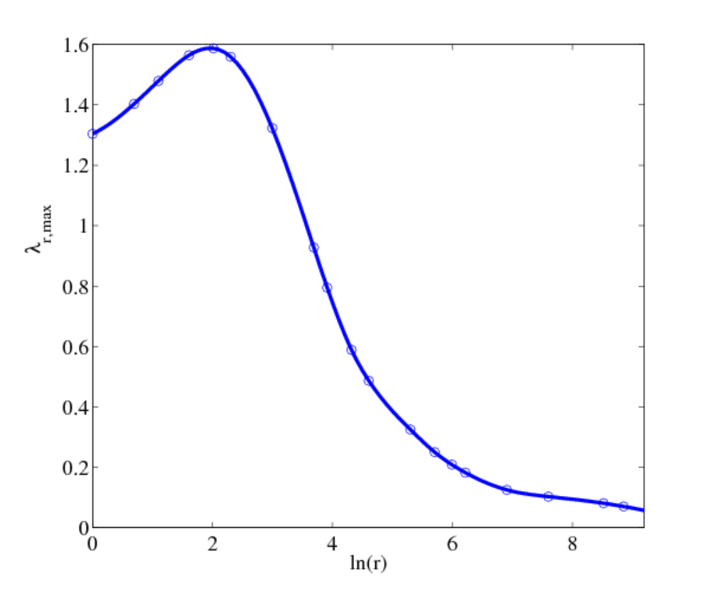
For large $r$ -values, the maximum growth rate decreases upon decreasing $r$ . This is not surprising: a decreasing value of $r$ implies that the density of the liquid approaches that of the gas, and thus the liquid has less inertia. The interface is then expected to be less stable. The plot in Fig. 12 (b) neatly sums up this dependence. However, for smaller $r$ -values $r\apprle 10$ , this dependence is reversed. This is explained by the energy budget in Tab. 3, where the energy decomposition at the maximum growth rate is shown, as a function of $r$ . The principal source of instability is the $TAN$ term, consistent

$r$	$\alpha$	$KIN_{G}$	$KIN_{L}$	$REY_{L}$	$REY_{G}$	$DISS_{L}$	$DISS_{G}$	$NOR$	$TAN$
1000	20	0.18	0.82	2.34	-11.90	-4.28	-57.42	-2.73	74.99
100	7.1	0.78	0.22	0.20	-2.60	-0.60	-14.21	-0.54	18.75
5	4.2	0.96	0.04	0.00	0.38	-0.35	-3.55	-0.13	4.65
1	3.9	0.99	0.01	0.00	0.32	-0.52	-4.26	-0.11	5.56

Table 3: Energy budget for the most dangerous mode as a function of

r

, for

Re_{0}=10^{3}

\delta=0.05

, and

m=55

. In general, there are two terms contributing to the instability: one interfacial, and one due to effects in the liquid layer. As

r

is reduced, the latter term diminishes importance, thus removing one of the sources of instability.

with a viscosity-contrast instability. Note that the term $REY_{L}$ is positive too, although this contribution diminishes with decreasing $r$ , so removing a source of instability and thus reversing the monotone dependence of the growth rate (at large $r$ , the growth rate decreases with increasing $r$ ). As $r$ decreases further (in particular, for $r=1$ , $5$ ), there is a destabilizing net input of energy into the perturbations from the $REY_{G}$ term, which implies that the critical-layer mechanism plays a secondary role.

These findings raise two questions. Is the turbulence model valid at these fast wave speeds? Is our base-state model valid at these low values of $r$ ? Now when the critical-layer mechanism is relevant, the dynamically important region moves into the bulk of the gas flow (away from the interface). It is possible that this region will coincide with that part of the gas domain where the rapidity of advection dominates over the eddy turnover time (see Sec. III). Thus, in this case, rapid-distortion effects may be important. These effects may alter both the growth rate and the structure of the wave-induced velocity field, and will be considered in future work, in a parametric study similar to this one. The second question concerns the wall-interface equivalence in the base-state model. This assumption was used in choosing the exponent in the wall function. Such an equivalence is only valid for large density contrasts. However, this is a relatively unimportant ingredient in the model, since it determines the second-order term (but not the first-order term) in the Taylor expansion of the base-state velocity near the interface $z=0$ . Thus, this equivalence assumption is unlikely to affect the development of fast waves as $r\downarrow 1$ . Having verified the effect of density stratification on the character of the instability, consistent with our analysis in Sec. II, we now perform a more systematic analysis on the effects of the Froude and Weber numbers on the instability.

We perform a parameter study based on the inverse Froude number $Fr$ in Fig. 13, wherein $Fr$ is varied around the reference value $Fr_{0}$ given by Eq. (30), at fixed density ratio and Reynolds number.

As expected, increasing $Fr$ is stabilizing; such an increase also leads to faster waves, and $c_{r}/U_{0}\apprge 1$ in a range of wavenumbers where the interface is unstable. In Fig. 14 we demonstrate the effects varying the inverse Weber number $S$ relative to the reference value $S_{0}$ (Eq. (30)), at fixed Reynolds number.

As expected, increasing $S$ is stabilizing, and leads to faster waves. However, the fast waves are stable, while the slower waves are unstable. This is in contrast to Fig. 14, where increasing $Fr$ led to fast, unstable waves. This difference can be readily understood by recourse to the free-surface formula (22), here recalled to be

\frac{c_{\mathrm{r}}}{U_{0}}\approx\sqrt{\frac{Fr}{r+1}\frac{1}{\tilde{\alpha}}+\frac{S}{r+1}\tilde{\alpha}}\sqrt{\tanh\left(\tilde{\alpha}\alpha\right)}.

The effects of varying $S$ in this equation are felt at large wavenumbers, while the effects of varying $Fr$ are more significant at smaller wavenumbers. Since the instability attains maximum growth at $\left(\ell/d_{L}\right)\approx 1$ – $10$ , it is the variation in $Fr$ that is prominent in

$Fr$	$S$	$\alpha$	$KIN_{G}$	$KIN_{L}$	$REY_{L}$	$REY_{G}$	$DISS_{L}$	$DISS_{G}$	$NOR$	$TAN$
$Fr_{0}$	$S_{0}$	20	0.18	0.82	2.34	-11.90	-4.28	-57.42	-2.73	74.99
$Fr_{0}$	10 $S_{0}$	3	1.00	1.00	0.00	-15.24	-2.72	-65.40	-6.78	91.14
$Fr_{0}$	$20S_{0}$	2	1.00	0.00	0.00	-33.29	-6.00	-155.23	-13.22	208.74
$0.1Fr_{0}$	$S_{0}$	10	0.00	1.00	0.00	-10.22	-0.53	-39.06	-2.22	53.04
$10Fr_{0}$	$S_{0}$	30	-3.16	2.16	0.00	0.04	-0.89	-1.53	-0.63	2.00

Table 4: Energy budgets for the parameter study in which

S

and

Fr

are varied, at fixed density ratio

r

. We have set

Re_{0}=1000

\left(m,r,\delta\right)=\left(55,1000,0.05\right)

, and we have taken the reference values

Fr_{0}=3.7809\times 10^{6}\left(r-1\right)/Re_{0}^{2}

and

S_{0}=1.1420\times 10^{7}/Re_{0}^{2}

. In all cases considered, and for both slow and fast waves, the instability is due to the viscosity-contrast mechanism.

the wavenumber range of instability. Thus, it is likely to be a shift in $Fr$ , rather than $S$ , that precipitates a change in the character of the unstable interfacial waves. In Tab. 4 we verify that it is the viscosity-contrast mechanism, and not the critical-layer mechanism, that is at work in each case of instability studied, in spite of the change in the wave speed. Careful parameter tuning is thus required to observe the critical-layer instability, which was highlighted in Fig. 12 and Tab. 3.

Finally, we study the effect of varying $Re_{0}$ in Fig. 15. The maximum growth rate and the cutoff wavenumber are both shifted to higher values with increasing

$Re_{0}$ . Typical values of the wave speed are higher for smaller values of $Re_{0}$ , as predicted by the formula for free-surface waves (21). However, for unstable waves, that is, for $\alpha$ less than the cutoff wavenumber, the wave speed $c_{\mathrm{r}}/U_{0}$ is less than unity, confirming that these are in fact slow waves. Two further issues arise when studying the $Re_{0}$ -dependence of the stability. First, upon decreasing $Re_{0}$ , the lower critical wavenumber shifts from $\alpha_{\mathrm{cl}}=0$ to some finite value $\alpha_{\mathrm{cl}}>0$ . This suggests that for a given parameter set $\left(m,r,\delta,Re_{0}^{2}S,Re_{0}^{2}Fr\right)$ , there is a critical Reynolds number for stability.

This is demonstrated in Fig. 16, where the critical Reynolds number is $Re_{0\mathrm{c}}\approx 750$ . In a later section, we use this result as a means of verifying our model against experiments, since the critical Reynolds number for the onset of instability is readily measured. The second issue concerns the development of a second unstable mode at higher Reynolds numbers, as demonstrated in Fig. 16 (b). This is the so-called internal mode, which we now investigate in detail.

IV.2 The internal mode

We examine the properties of the second unstable mode observed in Fig. 16 (b). We first of all examine the energy budget at $\alpha=25$ , for both unstable modes. This is shown in Tab. 5.

$\alpha$	$\lambda_{\mathrm{max}}$	$KIN_{G}$	$KIN_{L}$	$REY_{L}$	$REY_{G}$	$DISS_{L}$	$DISS_{G}$	$NOR$	$TAN$
25	0.77	0.85	0.15	0.45	-9.57	-0.41	-36.96	-1.17	48.67
25	0.15	0.15	0.85	3.80	-9.98	-0.80	-26.46	-0.18	34.62

Table 5: Energy budget of the interfacial and internal modes at

\alpha=25

. Here we have set

\left(m,r,\delta,Re_{0}\right)=\left(55,1000,0.05,2000\right)

. The values of

Fr

and

S

by Eq. (30). Both modes enjoy destabilizing contributions from

TAN

and

REY_{L}

, although this latter contribution is much larger for the internal mode.

As usual, the first mode, associated with the eigenvalue branch that has interested us until now, derives all but a small fraction of its destabilizing energy from the $TAN$ term, which we have identified as a work done by the tangential stress on the interface. This term is positive when $m>1$ , and we designate this mode the ‘interfacial’ mode. The second mode derives the majority of its destabilizing energy from this source too, although the term

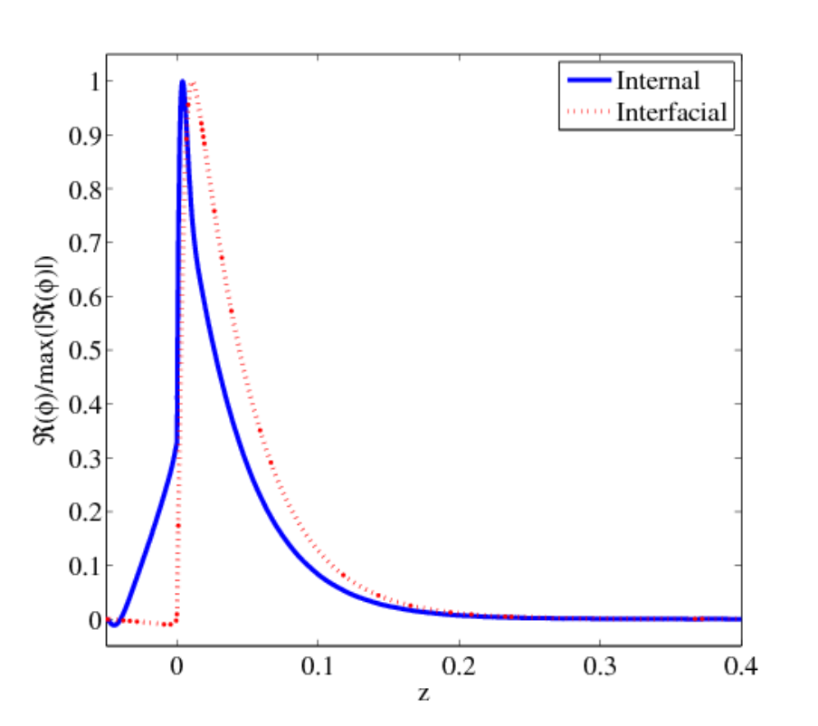
$REY_{L}$ is now more important. Thus, the transfer of energy from the mean flow in the liquid, to the perturbation flow, is important. We therefore designate this mode the ‘internal’ mode. This justification is strengthend further by examination of the streamfunction and wave Reynolds stress function associated with these modes, shown in Fig. 17. Figure 17 (a) shows the streamfunction for these two modes. The streamfunction of the internal mode possesses a large non-zero component in the liquid, in contrast to that of the interfacial mode. This gives rise to significant flow in the liquid, and hence gives an important contribution to the transfer term $REY_{L}$ . The development of a larger transfer term is shown in Fig. 17, where we examine the wave Reynolds stress. This is the function

	$\displaystyle\tau_{\mathrm{wave}}^{(i)}\left(z\right)$	$\displaystyle=$	$\displaystyle-r_{i}\int_{0}^{\ell}\delta u_{i}\left(x,z\right)\delta w_{i}\left(x,z\right)\frac{\mathrm{d}U_{i}^{(0)}}{\mathrm{d}z}\mathrm{d}x,\qquad i=L,G$
	$\displaystyle REY_{L}$	$\displaystyle=$	$\displaystyle\int_{-d_{L}}^{0}\tau_{\mathrm{wave}}^{(L)}\left(z\right)\mathrm{d}z.$

Clearly, $REY_{L}$ is much larger for the internal mode, thus confirming the importance of the dynamics of the liquid layer for the development of this secondary instability. Moreover, the critical layer of the internal mode is in the liquid, a fact that has been used in the past to justify its designation as ‘internal’ (Miesen and Boersma, 1995) ( $U\left(0\right)=0.92$ , and $c_{\mathrm{r}}=0.25$ at $\alpha=25$ for the internal mode).

The existence of a second unstable mode implies the possibility of mode competition, in which the most dangerous mode changes type, from being interfacial to internal. In Figs. 18–19 we demonstrate how this competition can be achieved by decreasing $m$ . This is expected to reduce the importance of the interfacial mode relative to the internal mode, since $TAN\propto m-1$ .

The figure does indeed confirm a change in the character of the most dangerous mode as $m$ is reduced: when $m$ is reduced from $20$ to $5$ , the most dangerous mode becomes internal. Note that this crossover depends not only on $m$ , but also on $Re_{0}$ : we need first of all to identify a value of $Re_{0}$ for which the internal mode is positive, and then carefully select $m$ to observe mode competition. Now a similar modal competition has been observed in two-phase mixing layers by Yecko et al. (2002), where again, the mode competition is a function of the viscosity contrast. What these examples share is the control of the modal competition by a parameter that requires a change in the properties of the two fluids under

investigation. There does however, exist a situation in which the mode competition can be engendered by a change in the flow properties (more precisely, a change in the properties of the turbulence), rather than in the fluid properties. It is to this example that we now turn.

IV.3 Modelling surface roughness

In this section we examine the effect of surface roughness on the internal and interfacial modes. Surface roughness is modelled by two distinct approaches. Now it is not inconsistent to examine the effects of surface roughness on wave growth: the origin of the surface roughness is not found in the waves we study, but rather in instantaneous pressure fluctuations at the interface that give rise to a roughened interface, where the vertical extent of the roughness elements is proportional to the strength of these pressure fluctuations. Such fluctuations appear in the work of Phillips (1957), and direct numerical simulations by Lin et al. (2008) indicate that these pressure fluctuations are a precursor to the exponential wave growth we have described here. As mentioned in Sec. II, we have two distinct models for the surface roughness. In the first

case, we use the smooth-interface model, with a reduced viscous sublayer thickness. Such an approach has been used before (Morland and Saffman, 1993), where it was observed that the reduced viscous sublayer produces a reduced wave growth rate. The second model we use is a modified version of that of Biberg (2007), where the eddy-viscosity contains an explicit roughness parameter $K=\ell_{\mathrm{i}}/\left(\kappa h\right)$ , where $\ell_{\mathrm{i}}$ is the mean height of the roughness elements. We compare these two approaches in this section.

Fig. 20 shows the effect of the viscous-sublayer thickness on the stability. The growth rate of the interfacial and internal modes is shown for viscous-sublayer thicknesses $5d_{*}$ , $2d_{*}$ , and $d_{*}$ . These different values are obtained from the base-state model by changing the Van Driest coefficient $A_{\mathrm{vd},\mathrm{i}}$ . Here, $d_{*}=\nu_{G}/U_{*\mathrm{i}}$ is the wall unit based on the interfacial friction velocity $U_{*\mathrm{i}}$ . From the figure, we see that decreasing the viscous sublayer thickness decreases the maximum growth rate of both modes.

Next, we turn to the Biberg model of interfacial roughness.

Fig. 21 shows the growth rate as a function of the roughness parameter $K$ . As $K$ increases, the maximum growth rate of the interfacial mode shrinks dramatically, while the maximum growth rate of the internal mode increases slightly. This change is sufficient to promote the maximum wavenumber-growth rate pair on the internal branch, $\left(\alpha_{\mathrm{max},\mathrm{int}},\lambda_{\mathrm{max},\mathrm{int}}\right)$ , to the status of most dangerous mode. This crossover occurs for $K\apprge 0.001$ , as shown in Fig. 18 (b).

In Fig. 21, the dispersion curve of the internal mode possesses a local minimum near $\alpha\approx 20$ , similar to Fig. 18 (c). To verify that this is not due to a crossover between the second and third modes, we have plotted the three least negative modes for $K=0.005$ in Fig. 22 (a). The second and third least negative modes are well separated and a crossover effect is thus ruled out. Figs. 22 (b) and (c) are plots of the wave speed for the internal and interfacial modes: the continuity of these curves confirms that no crossover effect is taking place. Note, however, that the wave speeds of the second and third most dangerous modes intersect close to the point where the internal mode has its local minimum. Such phenomena often occur in modal coalescence (Shapiro and Timoshin, 2005). Note finally that $c_{\mathrm{r}}-U_{\mathrm{int}}$ is negative for the internal mode, which shows that the critical layer is in the liquid for the internal mode.

Since the results in Figs. 20 and 21 are not identical, the two models of interfacial roughness discussed here are obviously inequivalent. Which, therefore, is the correct description? Reducing the depth of the viscous sublayer, and thus enhancing the extent of the logarithmic layer, is clearly a crude model for interfacial roughness. The level of detail in the Biberg model is superior, and the predictions of this model for a base state with finite roughness agree well with experiments, as explained in his paper (Biberg, 2007). Our prejudice is thus towards the latter model, and we therefore expect surface roughness to modify the stability properties of the system through mode competition. However, this contention must ultimately be confirmed by DNS, and by experiments. Although these studies are beyond the scope of the present work, we are able to test the predictions of the flat-interface model against experiments, which we do in the next section.

V Comparison with other work

In this section, we compare our results with some of the experimental data from the literature, in particular the work of Cohen and Hanratty (1965), and Craik (1966). We also compare our findings with a model that is frequently used in practical applications to predict flow-regime transitions, namely the viscous Kelvin–Helmholtz theory. To do this, we refer to Fig. 16 (a), which highlights the importance of the Reynolds number in the stability analysis. In that figure, the Reynolds number is varied and the other parameters are held fixed. For sufficiently large values of $Re_{0}$ , the dispersion curve associated with the interfacial mode is paraboloidal, with critical wavenumbers at $\alpha_{\mathrm{c},\mathrm{l}}=0$ , and $\alpha_{\mathrm{c},\mathrm{u}}>0$ . As the Reynolds number decreases, the the growth rate develops an intermediate critical wavenumber $\alpha_{\mathrm{c},\mathrm{u}_{0}}$ , where $0<\alpha_{\mathrm{c},\mathrm{u}_{0}}<\alpha_{\mathrm{c},\mathrm{u}}$ . At a critical $Re_{0}$ -value, the maximum growth rate is zero, and thus the intermediate critical wavenumber is simultaneously a maximum, and a zero, of the function $\lambda_{\mathrm{r}}\left(\alpha\right)$ . Finally, below this critical $Re_{0}$ -value, the growth rate is negative everywhere. The experimental works we reference involve a similar path through paramter space.

V.1 Comparison with experiments

Cohen and Hanratty (1965) report critical Reynolds numbers for millimetre-thick liquid films. They observe the development of two-dimensional waves above a critical Reynolds number. They call these waves ‘fast’, in the sense they move at a velocity that exceeds the interfacial velocity.

	$d_{L}$ (mm)	$Re_{CH}$	$Re_{CH}$ (exp)	$c_{\mathrm{r}}/\overline{U}_{G}$	$c_{\mathrm{r}}/\overline{U}_{G}$ (exp)	$\ell$ (inches)	$\ell$ (inches,exp)
(1)	1.89	3810	4050	0.13	0.08	1.1	0.9
(2)	3.54	2650	2760	0.15	0.15	0.7	1.2
(3)	4.91	1930	1980	–	0.19	0.9	–

$\alpha$	$KIN_{G}$	$KIN_{L}$	$REY_{L}$	$REY_{G}$	$DISS_{L}$	$DISS_{G}$	$NOR$	$TAN$
5.5	0.99	0.01	4.58	1.91	-21.32	-31.44	-1.55	48.82

Table 6: Comparison with the work of Cohen and Hanratty (1965). There is excellent agreement between the theory and the experiments. One should note however, that the experiments carry a margin of error of up to

20\%

. Thus, the agreement between the critical Reynolds numbers is both indicative of the correctness of our theory, and possibly a little fortuitous. The sub-table is a theoretical energy-budget calculation related to experiment (3). The instability is viscosity-induced, although there are contributions from

REY_{L}

and

REY_{G}

too.

These waves are, however, in our classification, ‘slow’ (or on the boundary beween ‘slow’ and ‘fast’), since the theoretical values computed are $c_{\mathrm{r}}/U_{0}\apprle 1$ , and thus the viscosity-contrast instability is expected. We show a comparison between the theoretical predictions of our model and the measurements of Cohen and Hanratty in Tab. 6. Our estimates for the critical Reynolds number $Re_{CH}=\rho_{G}h\overline{U}_{G}/\mu_{G}$ are in close agreement with the experimental values. We are mindful, however, that the margin of error

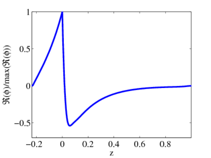
stated in the experiment is between $10\%$ and $20\%$ . We have also compared our theoretical model with the measurements of the critical wavelength and wave speed. There is excellent agreement between the theoretical and experimental values for the wave speed. The spread in values of the critical wavelength is larger, although this is acceptable, in view of the large error attached to the experimental measurements. The energy budget in Tab. 6 is based on a theoretical calculation, with parameters taken from experiment (3). The corresponding streamfunction and the wave Reynolds stress function are presented in Fig. 23. The instability is confirmed to be due to the viscosity-contrast mechanism.

Craik (1966) performs a similar experiment with liquid films thinner than those found in Cohen and Hanratty. He reports critical conditions for the generation of unstable waves. The trend in the data agrees with that in the theoretical calculations, although the quantitative agreement is poor. Craik explains that waves

	$d_{L}$ (mm)	$Re_{Cr}$	$Re_{Cr}$ (exp)
(1.1)	0.128	$20$	$30$
(1.2)	0.230	$68$	$61$
(1.3)	0.218	$66$	$71$
(1.4)	0.355	$110$	$140$
(1.5)	0.307	$94$	$140$

	$d_{L}$ (mm)	$Re_{Cr}$	$Re_{Cr}$ (exp)	$c_{\mathrm{r}}/U_{\mathrm{int}}$	$c_{\mathrm{r}}/U_{\mathrm{int}}$ (exp)
(2.1)	0.535	$35$	$94$	1.1	1.75
(2.2)	0.665	$50$	$89$	1.0	1.9
(2.3)	0.820	$56$	$91$	1.1	1.8

Table 7: Comparison with Table 1 (p. 375) and Table 2 (p. 378) in the work of Craik (1966). There is good agreement between the theory and the experiment in the first case, and only very rough agreement in the second case. As explained in the experimental paper, a sharp transition to wavy flows was not observed in this second case, which explains these quantitative differences. We do not refer to experiments (2.4)–(2.5), wherein our model predicts laminar gas flow.

are observed for film thickness below that quoted in experiment (1.1), although the uniform thin film of liquid is difficult to maintain under these conditions. It is possible that the thinness of the film inhibits precision in the measurement at film thickness above this lower bound too. Craik also explains that accurate measurements of wave speed were difficult owing to the long wavelengths of the observed waves (compared to the channel length). These are sources of error that explain why there is only qualitative agreement between the theoretical and experimental data.

	$\alpha$	$KIN_{G}$	$KIN_{L}$	$REY_{L}$	$REY_{G}$	$DISS_{L}$	$DISS_{G}$	$NOR$	$TAN$
(1.5)	0.3	1.00	0.00	0.00	-165.56	-2.47	-1359.25	-0.09	1528.37
(2.1)	0.02	1.00	0.00	0.00	-45.06	-3.23	-701.34	-0.14	750.76

Table 8: Theoretical energy-budget calculations related to experiments (1.5) and (2.1) of Craik. The instability is viscosity-induced, and there are no other contributions to the instability, unlike in the Cohen data.

We also perform theoretical calculations based on the parameters in experiments (1.5) and (2.3), to examine that character of the unstable waves. We provide the energy budgets associated with these calculations in Tab. 8. The instability is interfacial: the contribution from $REY_{L}$ and $REY_{G}$ present in the Cohen data are absent here. This makes sense: $REY_{L}$ should be negligible because the liquid layer is so thin and thus $\phi_{L}$ cannot contribute meaningfully to the dynamics, while $REY_{G}$ is unimportant because the waves are slow ( $c_{\mathrm{r}}/U_{0}$ is $O(10^{-2})$ or $O(10^{-1})$ for the film thicknesses and Reynolds numbers considered).

V.2 Comparison with Viscous Kelvin–Helmholtz theory

In this section, we compare our predictions with those obtained using viscous Kelvin–Helmholtz theory (Barnea, 1991). This is a simplified theory for the interfacial instability of two-phase turbulent flow, and takes account of turbulence in either or both phases. It is commonly used in one-dimensional models for large-scale stratified and slug-flow predictions. The velocity field enters only through the liquid- and gas-average values, $u_{L}$ and $u_{G}$ , while the cross-sectional area fractions $\epsilon_{L}=d_{L}/\left(d_{L}+d_{G}\right)$ and $\epsilon_{G}=d_{G}/\left(d_{L}+d_{G}\right)$ also play a role. Then, the complex frequency $\omega$ is obtainable from a quadratic equation:

\omega^{2}-2\left(x_{0}\alpha-x_{1}i\right)\omega+\left(x_{2}\alpha^{2}-x_{3}\alpha^{4}-ix_{4}\alpha\right)=0,

where

$\displaystyle\rho_{*}$	$\displaystyle=$	$\displaystyle\frac{\rho_{L}}{\epsilon_{L}}+\frac{\rho_{G}}{\epsilon_{G}},$
$\displaystyle x_{1}$	$\displaystyle=$	$\displaystyle\frac{1}{\rho_{*}}\left(\frac{\rho_{L}u_{L}}{\epsilon_{L}}+\frac{\rho_{G}u_{G}}{\epsilon_{G}}\right),$
$\displaystyle x_{2}$	$\displaystyle=$	$\displaystyle-\frac{S_{\mathrm{\mathrm{i}}}}{2\rho_{*}A}\left(\frac{1}{\epsilon_{L}}+\frac{1}{\epsilon_{G}}\right)\left(\frac{1}{\epsilon_{G}}\frac{\partial\tau_{\mathrm{i}}}{\partial{u_{G}}}-\frac{1}{\epsilon_{L}}\frac{\partial\tau_{\mathrm{i}}}{\partial{u_{L}}}+\frac{1}{\epsilon_{L}}\frac{\partial\tau_{\mathrm{i}L}}{\partial{u_{L}}}-\frac{1}{\epsilon_{G}}\frac{\partial\tau_{\mathrm{i}L}}{\partial{u_{G}}}\right),$
$\displaystyle x_{3}$	$\displaystyle=$	$\displaystyle\frac{1}{\rho_{*}}\left[\frac{\rho_{L}u_{L}^{2}}{\epsilon_{L}}+\frac{\rho_{G}u_{G}^{2}}{\epsilon_{G}}-g\left(\rho_{L}-\rho_{G}\right)\left(d_{L}+d_{G}\right)\right],$
$\displaystyle x_{4}$	$\displaystyle=$	$\displaystyle\frac{\sigma}{\rho_{*}}\left(d_{L}+d_{G}\right),$
$\displaystyle x_{5}$	$\displaystyle=$	$\displaystyle\frac{S_{\mathrm{\mathrm{\mathrm{i}}}}}{\rho_{*}A}\left(\frac{\partial\tau_{\mathrm{i}L}}{\partial\epsilon_{L}}-\frac{\partial\tau_{\mathrm{i}}}{\partial\epsilon_{L}}+\frac{u_{G}}{\epsilon_{G}}\frac{\partial\tau_{\mathrm{i}L}}{\partial{u_{G}}}-\frac{u_{G}}{\epsilon_{G}}\frac{\partial\tau_{\mathrm{i}}}{\partial{u_{G}}}-\frac{u_{L}}{\epsilon_{L}}\frac{\partial\tau_{\mathrm{i}L}}{\partial{u_{L}}}+\frac{u_{L}}{\epsilon_{L}}\frac{\partial\tau_{\mathrm{i}}}{\partial{u_{L}}}\right),$

and where the viscous stresses are modelled as

$\displaystyle\tau_{L}$	$\displaystyle=$	$\displaystyle\tfrac{1}{2}f_{L}\rho_{L}u_{L}^{2},\qquad f_{L}=C_{L}\left(\frac{D_{L}u_{L}}{\nu_{L}}\right)^{-n_{L}},\qquad D_{L}=4d_{L},$
$\displaystyle\tau_{G}$	$\displaystyle=$	$\displaystyle\tfrac{1}{2}f_{G}\rho_{G}u_{G}^{2},\qquad f_{G}=C_{G}\left(\frac{D_{G}u_{G}}{\nu_{G}}\right)^{-n_{G}},\qquad D_{G}=2d_{G},$
$\displaystyle\tau_{\mathrm{i}}$	$\displaystyle=$	$\displaystyle\tfrac{1}{2}f_{\mathrm{i}}\rho_{G}\left(u_{G}-u_{L}\right)\|u_{G}-u_{L}\|,$
$\displaystyle\tau_{\mathrm{i}L}$	$\displaystyle=$	$\displaystyle\frac{\tau_{L}\epsilon_{G}-\tau_{G}\epsilon_{L}}{\epsilon_{L}+\epsilon_{G}}.$

The coefficients $C_{G}$ and $C_{L}$ both take the value $0.046$ for turbulent flow and $16$ for laminar flow, while $n_{L}$ and $n_{G}$ both take the value $0.2$ for turbulent flow, and $1.0$ for laminar flow. Finally, the interfacial friction factor $f_{\mathrm{i}}$ is assumed to be constant and equal to $0.0142$ (see Barnea (1991)). We plot the stability boundary predicted by this theory in Fig. 24, and compare the results with the Craik data for the $6\,\mathrm{in.}$ channel (Tab. 7), and with a curve fit based on a number of points obtained from our theoretical calculations. The viscous Kelvin–Helmholtz model overpredicts the critical Reynolds number compared with both the data of Craik and our theoretical model by an order of magnitude (Fig. 24), which casts doubt on the usefulness of such a depth-averaged model. Our model gives better agreement with the data of Craik, although we are mindful of the uncertainty in these experimental data. Nevertheless, both our theoretical calculations and the experimental data demonstrate the unstable-stable-unstable transition that arises when the film depth is increased, holding the Reynolds number fixed. This is the statement that our theoretical curve in Fig. 24 is non-monotonic (the non-monotonicity in the model curve is masked somewhat by the large scale necessary to show the VKH results in the same figure). In conclusion, the qualitative agreement obtained here, together with the good agreement obtained relative to the Cohen data, inspires confidence in our model, while the poor agreement between our data and the predictions of the viscous Kelvin–Helmholtz theory calls into question the validity of this depth-averaged model, at least for the kind of thin-film waves studied here.

VI Conclusions

In this paper, we have investigated the stability of an interface separating a thin laminar liquid layer from a turbulent gas in a channel. We have approached this problem in two steps: first by generalizing the model of Biberg (2007) to describe the interfacial and wall zones in pressure-driven two-phase channel flow, and second by studying the linear stability of this state using an Orr–Sommerfeld analysis of the Reynolds-averaged Navier–Stokes equations. Our model has enabled us to investigate the stability of the interface as a function of various parameters. In general, the interface becomes unstable due to a mismatch between the viscosities in the liquid and the gas. In this work, we have taken into account the perturbation turbulent stresses (PTS) using two distinct models: in both cases, these stresses have only a quantitative effect on the stability results for the thin liquid layers; for the eddy-viscosity model of the PTS, this effect is particularly small. These stress contributions are therefore ignored throughout the work. We have provided an explanation for this null result using an analogy with non-Newtonian fluids. This work builds upon previous work in the field (notably that of Miesen and co-workers (Miesen and Boersma, 1995; Boomkamp and Miesen, 1996; Boomkamp et al., 1997), and Kuru et al. (1995)) by developing an accurate base-state model, validated against numerous experiments and direct-numerical simulations, and by accounting for the PTS. These efforts result in excellent agreement with the relevant experiments (Craik, 1966; Cohen and Hanratty, 1965).

Our linear stability analyses evince a definition of slow and fast waves. A slow wave is one for which the instability is driven by the viscosity contrast across the interface; a fast wave derives its energy of instability from the critical layer. The phase speed $c_{\mathrm{r}}$ of a slow waves satisfies $c_{\mathrm{r}}/U_{0}\apprle 1$ , where $\rho_{G}U_{0}^{2}=h|\partial p/\partial x|$ . We have carried out a parameter study to find ways of controlling the wave speed. The inverse Froude, inverse Weber, and density numbers control the wave speed, as suggested by the formula for free-surface waves in a liquid layer. However, in all cases considered, the waves are slow. For certain values of the triple $\left(r,Fr,S\right)$ , there is a critical-layer contribution to the instability, although this is marginal.

For certain parameter values, we also observe a positive growth rate for the so-called internal mode, associated with instability that is due both to the shear content of the liquid and to the tangential stress at the interface. By a judicious choice of parameters (in particular, for small viscosity ratios), the internal mode can be made to dominate over the interfacial mode, and gives rise to mode competition. To engineer mode competition in this way, it is necessary to modify the properties of the two fluids. However, by increasing the level of turbulence, the flat interface roughens, and this also has the effect of diminishing the interfacial mode relative to the internal mode. Morland and Saffman (1993) have explained previously how roughness can reduce the growth rate of the wave; here we go further and conjecture that this mechanism can, in addition, engender mode competition. However, this result is rather conjectural, and we simply mention it as a route for future experiments.

Acknowledgements

This work has been undertaken within the Joint Project on Transient Multiphase Flows and Flow Assurance. The Authors wish to acknowledge the contributions made to this project by the UK Engineering and Physical Sciences Research Council (EPSRC) and the following: – Advantica; BP Exploration; CD-adapco; Chevron; ConocoPhillips; ENI; ExxonMobil; FEESA; IFP; Institutt for Energiteknikk; PDVSA (INTEVEP); Petrobras; PETRONAS; Scandpower PT; Shell; SINTEF; StatoilHydro and TOTAL. The Authors wish to express their sincere gratitude for this support.

APPENDIX A

For further validation of the base state discussed in Sec. II, we compare our turbulence modelling with experimental data for flow past a wavy wall, obtained from the papers of Zilker et al. (1976), and Abrams and Hanratty (1985). The curvilinear coordinates necessary for this work were previously introduced by Benjamin (1958) $\,\dagger\,$ :^$*$^$*$footnotetext: $\dagger$ We thank S. Kalliadasis and D. Tseluiko for suggesting the application of this coordinate system to the problem.

	$\displaystyle\xi$	$\displaystyle=$	$\displaystyle x-ia\Phi,$
	$\displaystyle\eta$	$\displaystyle=$	$\displaystyle z-a\Phi,\qquad\Phi=e^{-\alpha z}e^{i\alpha x}.$		(A-1)

If the streamfunction has the form

\phi=\int_{0}^{\eta}U_{0}\left(s\right)ds+aF\left(\eta\right)e^{i\alpha\xi}

(where $U_{0}$ is the single-phase version of the base state in Eq. (12)), then the momentum-balance equation for $F$ is

	$i\alpha\left[\left(\partial_{\eta}^{2}-\alpha^{2}\right)F\left(\eta\right)-U_{0}^{\prime\prime}\left(\eta\right)F\left(\eta\right)\right]+\mathcal{C}=\frac{1}{Re_{0}}\left(\partial_{\eta}^{2}-\alpha^{2}\right)^{2}F\left(\eta\right)+\mathcal{R},$	(A-2a)
where $\mathcal{C}$ is the curvature-related term
	$\mathcal{C}=2i\alpha^{2}\,U_{0}^{\prime}\left(\eta\right)U_{0}\left(\eta\right)e^{-\alpha\eta}+\frac{1}{Re_{0}}e^{-\alpha\eta}\left[4\alpha^{2}U_{0}^{\prime\prime}\left(\eta\right)-2\alpha U_{0}^{\prime\prime\prime}\left(\eta\right)\right],$	(A-2b)
and $\mathcal{R}$ is the Reynolds-stress term:
	${\mathcal{R}}=\left(\partial_{\eta}^{2}+\alpha^{2}\right)\Big\{\mu_{T}\left[F^{\prime\prime}\left(\eta\right)+\alpha^{2}F\left(\eta\right)+2\alpha U_{0}^{\prime}\left(\eta\right)e^{-\alpha\eta}-2\alpha^{2}U_{0}\left(\eta\right)e^{-\alpha\eta}\right]\Big\}\\ +2e^{-\alpha\eta}\left[\alpha\tau_{0}^{\prime\prime}\left(\eta\right)-\alpha^{2}\tau_{0}^{\prime}\left(\eta\right)\right],\qquad\tau_{0}\left(\eta\right)=\mu_{T}\left(\eta\right)U_{0}^{\prime}\left(\eta\right).$	(A-2c)

The function $\mu_{T}\left(\eta\right)$ is the eddy viscosity. It is set to zero in the quasi-laminar case, and assigned the form of Eq. (6) if the perturbation turbulent stresses are considered. We solve Eqs. (A-2c) subject to the boundary conditions $F=F^{\prime}=0$ on $\eta=0$ and on $\eta=1$ , which are no-slip conditions on the perturbation $F$ . Although the no-slip condition on the upper boundary is at $z=1$ , not $\eta=1$ , these planes are close to one another: the physical boundary $z=1$ corresponds to an $\eta$ -value $1-ae^{-\alpha}e^{i\alpha x}$ , which is close to unity for large $\alpha$ -values. Thus, for simplicity, we impose a boundary condition at $\eta=1$ .

The solution of the boundary-value problem facilitates a comparison with experimental data. In this comparison, we use the quasi-laminar assumption: the eddy-viscosity terms $\mathcal{R}$ are set to zero, and turbulence enters only through the shape of the base state $U_{0}$ . To make an accurate comparison between the experiments and Eqs. (A-2c) we study the shear stress at the interface:

\tau_{0}=Re_{0}^{-1}\left(\phi_{zz}-\phi_{xx}\right)_{\eta=0}=\frac{ae^{i\alpha\xi}}{Re_{0}}\left[F^{\prime\prime}\left(0\right)+\alpha^{2}F\left(0\right)+2\alpha\left(Re_{*}^{2}/Re_{0}\right)\right].

(A-3)

We also study the phase shift between this stress function and the wave surface $a\Re\left[e^{i\alpha\xi}\right]$ . We examine the situation described by Fig. (5) in the work of Zilker et al. (1976), for which

a/H=0.003,\qquad\alpha H=13.3,\qquad Re_{*}=2270,

where $H=5.08\,\mathrm{cm}$ is the channel depth. We also look at Fig. (4) in the work of Abrams and Hanratty, where

a/H=0.007,\qquad\alpha H=2\pi,\qquad Re_{*}=1110,

where $H$ is the same is in the Zilker experiment. A comparison between theory and experiment is shown in Fig. A-1, where good agreement is obtained.

Note that in several crucial respects, the stability calculations performed in the main part of paper and the wavy-wall calculations performed in this Appendix are different. In the case of small-amplitude waves on an interface, the growth of waves is understood through a linear stability analysis. Thus, the amplitude of the initial interfacial disturbance is assumed to be small, and functions as a small parameter in a linear stability analysis. In contrast, the amplitude of the wavy wall is not infinitesimally small, and it is the finiteness of this amplitude that gives rise to the curvature terms in the equations (A-2c), which in turn affects the distribution of stress at the interface. Furthermore, the wave speed in the wavy-wall calculation is a known parameter. In the linear stability analysis, it is determined as the solution of an eigenvalue problem. It might be tempting to guess the wave speed in the case of interfacial waves by recourse to the free-surface formula (21) but our linear stability analysis shows that the $\alpha$ -range of maximal wave growth is precisely that range where this formula is least reliable (See Fig. 8). Thus, a key difference between these two calculations is that in the wavy-call case, $c$ is a parameter; in the wavy-interface case, it must be determined from other parameters. One similarity between the calculations is the shape of the streamfunction. In the two-phase calculation, the shape of the streamfunction in the upper layer is similar to that obtained from the wavy-wall calculation (Figs. A-1 (b) and A-1 (d)). This is a consequence of the boundary conditions, which impose severe limitations on the shape of the streamfunction. In conclusion, the wavy-wall calculation, because it assumes that the wave speed is a parameter, is an incomplete model for two-phase wavy interface calculations. It is, however, a testbed for verifying the turbulence modelling of the basic state.

References

Abrams and Hanratty (1985) J. Abrams and T. J. Hanratty. Relaxation effects observed for turbulent flow over a wavy surface. J. Fluid Mech., 151:443–455, 1985.
Adjoua and Magnaudet (2009) S. Adjoua and J. Magnaudet. Développement d’une méthode de simulation à un fluide d�écoulements diphasiques turbulents. In 19 $\,{}^{\text{\`{e}me}}$ Congrès Français de Mécanique, 2009.
Akai et al. (1980) M. Akai, A. Isoue, S. Aoki, and K. Endo. A co-current stratified air-mercury flow with wavy interface. Int. J. Multiphase Flow, 6:173–190, 1980.
Akai et al. (1981) M. Akai, A. Isoue, S. Aoki, and K. Endo. The prediction of stratified two-phase flow with a two-equation model of turbulence. Int. J. Multiphase Flow, 7:21–39, 1981.
Barnea (1991) D. Barnea. On the effect of viscosity on stability of stratified gas-liquid flow – Application to flow pattern transition at various pipe inclinations. Chem. Eng. Sci., 46:2123–2131, 1991.
Belcher and Hunt (1993) S. E. Belcher and J. C. R. Hunt. Turbulent shear flow over slowly moving waves. J. Fluid Mech., 251:109–148, 1993.
Belcher et al. (1994) S. E. Belcher, J. A. Harris, and R. L. Street. Linear dynamics of wind waves in coupled turbulent air-water flow. Part 1. Theory. J. Fluid Mech., 271:119–151, 1994.
Benjamin (1958) T. B. Benjamin. Shearing flow over a wavy boundary. J. Fluid Mech., 6:161–205, 1958.
Biberg (2007) D. Biberg. A mathematical model for two-phase stratified turbulent duct flow. Multiph. Sci. Techn., 19:1–48, 2007.
Boeck et al. (2007) T. Boeck, J. Li, E. Lopez-Pages, P. Yecko, and S. Zaleski. Ligament formation in sheared liquid-gas layers. Theor. Comput. Fluid Dyn., 21:59–76, 2007.
Boomkamp and Miesen (1996) P. A. M. Boomkamp and R. H. M. Miesen. Classification of instabilities in parallel two-phase flow. Int. J. Multiphase Flow, 22:67–88, 1996.
Boomkamp et al. (1997) P. A. M. Boomkamp, B. J. Boersma, R. H. M. Miesen, and G. v. Beijnon. A Chebyshev collocation method for solving two-phase flow stability problems. J. Comput. Phys, 132:191–200, 1997.
Bradshaw (1974) P. Bradshaw. Possible origin of prandtl’s mixing-length theory. Nature, 249:135, 1974.
Chandrasekhar (1961) S. Chandrasekhar. Hydrodynamic and Hydromagnetic Stability. Dover, New York, 1961.
Cohen and Hanratty (1965) L. S. Cohen and T. J. Hanratty. Generation of waves in the concurrent flow of air and a liquid. A.I.Ch.E. Journal, 11:138, 1965.
Craik (1966) A. D. D. Craik. Wind-generated waves in thin liquid films. J. Fluid Mech., 26:369–392, 1966.
Fulgosi et al. (2002) M. Fulgosi, D. Lakehal, S. Banerjee, and V. De Angelis. Direct numericical simulations of turbulence in a sheared air-water flow with a deformable interface. J. Fluid Mech., 482:319–345, 2002.
Fuster et al. (2009) D. Fuster, A. Bague, T. Boeck, L. Le Moyne, A. Leboissetier, S. Popinet, P. Ray, R. Scardovelli, and S. Zaleski. Simulation of primary atomization with an octree adaptive mesh refinement and vof method. Int. J. Multiph. Flow, 35:550–565, 2009.
Hall-Taylor and Hewitt (1970) N. S. Hall-Taylor and G. F. Hewitt. Annular Two-Phase Flows. Pergamon Press, Oxford, 1970.
Ierley and Miles (2001) G. Ierley and J. Miles. On Townsend’s rapid-distortion model of the turbulent-wind-wave problem. J. Fluid Mech., 435:175–189, 2001.
Janssen (2004) P. A. E. M. Janssen. The interaction of ocean waves and wind. Cambridge University Press, Cambridge, UK, 2004.
Kuru et al. (1995) W. C. Kuru, M. Sangalli, D. D. Uphold, and M. J. McCready. Linear stability of stratified channel flow. Int. J. Multiphase Flow, 21:733–753, 1995.
Lin et al. (2008) M.-Y. Lin, C.-H. Moeng, W.-T. Tsai, P.P. Sullivan, and S.E. Belcher. Direct numerical simulation of wind-wave. J. Fluid Mech., 616:1–30, 2008.
Miesen and Boersma (1995) R. Miesen and B. J. Boersma. Hydrodynamic stability of a sheared liquid film. J. Fluid Mech., 301:175–202, 1995.
Miles (1957) J. W. Miles. On the generation of surface waves by shear flows. J. Fluid Mech., 3:185–204, 1957.
Miles (1962) J. W. Miles. On the generation of surface waves by shear flows. Part 4. J. Fluid Mech., 13:433–448, 1962.
Monin and Yaglom (1971) A. S. Monin and A. M. Yaglom. Statistical Fluid Mechanics: Mechanics of Turbulence. MIT Press, Cambridge, MA, 1971.
Morland and Saffman (1993) L. C. Morland and P. G. Saffman. Effect of wind profile on the instability of wind blowing over water. J. Fluid Mech., 252:383–398, 1993.
Náraigh and Spelt (2010) L. Ó Náraigh and P. D. M. Spelt. Interfacial instability of turbulent two-phase stratified flow: pressure-driven flow and non-newtonian layers. J. Non-Newt. Fluid Mech., 165:489–508, 2010.
Orr (1907a) W. M’F Orr. The stability or instability of the steady motions of a perfect liquid and of a viscous liquid. Part I. Proc. R. Irish Acad., 27:9–138, 1907a.
Orr (1907b) W. M’F Orr. The stability or instability of the steady motions of a perfect liquid and of a viscous liquid. Part II. Proc. R. Irish Acad., 27:69–138, 1907b.
Orszag (1971) S. A. Orszag. Accurate solution of the orr–sommerfeld stability equation. J. Fluid Mech., 50:689–703, 1971.
Özgen et al. (1998) S. Özgen, G. Degrez, and G. S. R. Sarma. Two-fluid boundary layer stability. Phys. Fluids, 10:2746–2757, 1998.
Phillips (1957) O. M. Phillips. On the generation of waves by turbulent wind. J. Fluid Mech., 2:417–445, 1957.
Pope (2000) S. B. Pope. Turbulent Flows. Cambridge University Press, Cambridge, UK, 2000.
Sahu et al. (2007) K. C. Sahu, P. Valluri, P. D. M. Spelt, and O. K. Matar. Linear instability of pressure-driven channel flow of a Newtonian and Herschel–Bulkley fluid. Phys. Fluids, 19:122101, 2007.
Shapiro and Timoshin (2005) E. Shapiro and S. Timoshin. On the patterns of interaction between shear and interfacial modes in plane air-water poiseuille flow. Proc. R. Soc. A, 461:1583, 2005.
Solbakken and Andersson (2004) S. Solbakken and H. I. Andersson. On the drag reduction mechanism in a lubricated turbulent channel flow. Int. J. Heat Fluid Flow, 25:618, 2004.
Spalart (1988) P. R. Spalart. Direct simulation of a turbulent boundary layer up to $r_{\theta}=1410$ . J. Fluid Mech., 187:61–98, 1988.
Sullivan et al. (2000) P. P. Sullivan, J. McWilliams, and C.-H. Moeng. Simulation of turbulent flow over idealized water waves. J. Fluid Mech., 404:47–85, 2000.
Townsend (1972) A. A. Townsend. Flow in a deep turbulent boundary layer over a surface distorted by water waves. J. Fluid Mech., 55:719–735, 1972.
Townsend (1980) A. A. Townsend. The response of sheared turbulence to additional distortion. J. Fluid Mech., 81:171–191, 1980.
Valluri et al. (2008) P. Valluri, P. D. M. Spelt, C. J. Lawrence, and G. F. Hewitt. Numerical simulation of the onset of slug initiation in laminar horizontal channel flow. Int. J. Multiph. Flow, 34:206–225, 2008.
Valluri et al. (2010) P. Valluri, L. Ó Náraigh, H. Ding, and P. D. M. Spelt. Linear and nonlinear spatio-temporal instability in laminar two-layer flows. J. Fluid Mech. (in press), 2010.
Willmarth et al. (1987) W. W. Willmarth, T. Wei, and C. O. Lee. Laser anemometer measurements of reynolds stress in a turbulent channel flow with drag reducing polymer additives. Phys. Fluids, 30:933, 1987.
Yecko et al. (2002) P. Yecko, S. Zaleski, and J.-M. Fullana. Viscous modes in two-phase mixing layers. Phys. Fluids, 14:4115, 2002.
Yiantsios and Higgins (1988) S. G. Yiantsios and B. G. Higgins. Linear stability of plane Poiseuile flow of two superposed fluids. Phys. Fluids, 31:3225–3238, 1988.
Yih (1967) C. S. Yih. Instability due to viscosity stratification. J. Fluid Mech., 27:337–352, 1967.
Zilker et al. (1976) D. P. Zilker, G. W. Cook, and T. J. Hanratty. Influence of the amplitude of a solid wavy wall on a turbulent flow. part 1. non-separated flows. J. Fluid Mech., 82:29–51, 1976.
Zou (1998) Q. Zou. A viscoelastic model for turbulent flow over undulating topography. J. Fluid Mech., 355:81–112, 1998.