Fighting decoherence in a continuous two-qubit odd or even parity measurement
with a closed-loop setup

It has been realized that measurements provide a powerful toolbox to manipulate the state of quantum systems in ways that might be difficult to achieve with standard interactions. An example is the possibility of quantum computing with only single photon sources, linear optics, and photo detectors [1]. A measurement may consist in observing a part of a larger system such as in several recent experiments preparing various quantum states of light by conditional detection of a small part of the light field [2, 3, 4]. Alternatively, one may use a probe to gain information about the state of a system as in atomic spin squeezing by use of Faraday rotation [5]. In the latter case, the measurement should ideally be constructed in such a way that the interaction between the probe and the system does not affect the time evolution of the measured observable.

A particularly interesting case arises, when the measured observable has degenerate eigenvalues, since one may then obtain partial information about the state of the system, while leaving a specific subspace unaffected. This opens the way to use measurements to prepare macroscopic quantum superposition states [6, 7] and to detect errors in quantum computations without destroying the quantum information stored in the qubits [8]. An example is the three-qubit bit-flip code, where each qubit is encoded in the two states $|000\rangle$ and $|111\rangle$ of three physical qubits, and a single bit-flip error can be detected by measuring the parity of qubits 1 and 2 and the parity of qubits 2 and 3. Other applications of parity measurements include entanglement generation [9], quantum computing [10], and state transfer [11].

Recently, it has been proposed to perform a continuous parity measurement on two qubits in a cavity quantum electrodynamics network by allowing a coherent state probe to interact sequentially with the two qubits and then measure the phase shift imposed on the probe light with a homodyne detector [12]. More precisely, each qubit is encoded in two ground state levels $|0\rangle$ and $|1\rangle$ of a single atom in a cavity, and the probe light couples the state $|1\rangle$ resonantly to an excited state $|e\rangle$. In the strong coupling limit, the vacuum Rabi splitting prevents the light from entering into the cavity if the atom is in the state $|1\rangle$ [13], and each interaction thus leaves the probe light unaffected except for a conditional phase shift of $\pi$ [14]. The measurement takes a finite amount of time due to uncertainties arising from shot noise, and it is suitable for continuous quantum error correction, where feedback is used to keep the state of the qubits within the code space as far as possible [15, 16]. Quantum error correction is often thought of as strong measurements followed by fast corrections, but continuous error correction contains some interesting aspects due to the intrinsic robustness of feedback control. In [17] a setup has been proposed in which the above interaction is used, but rather than detecting the probe field, the probe field is used in a feedback loop, which automatically corrects errors.

Independent of whether the probe field is detected or used for coherent feedback, it is important to minimize decoherence within the parity subspaces due to the interaction with the probe. The above scheme is sensitive to light field losses between and within the two cavities as well as to spontaneous emission from the excited state of each atom, arising because the field is not completely expelled when the coupling strength is finite. In the present paper we show that a slight change of the setup can decrease the rate of decoherence in the odd or the even parity subspace by about one order of magnitude. The basic idea is to allow the light field to interact several times with the two qubits by reflecting some of the light emerging from the second cavity back onto the input mirror of the first cavity as shown in Fig. 1. For the odd subspace (and $P=1$), the light field experiences a phase shift of $\pi$ for each round trip in the loop, and the resulting destructive interference between light fields having traveled a different number of round trips in the loop almost extinguishes the field. The difference between the field amplitudes obtained for the two possible states within the odd subspace is thus small, and this improves the robustness of the measurement with respect to loss. The destructive interference also decreases the field amplitudes inside the qubit cavities, which reduces the rate of spontaneous emission events and further decreases the decoherence rate. On the other hand, the sensitivity of the measurement is not decreased, since the even parity subspace leads to constructive interference in the loop, i.e., the phase of the output field differs by $\pi$ for the two subspaces as before. We note that the roles of the odd and the even parity subspaces could be exchanged by adding a phase shift of $\pi$ within the loop, but in the following we focus on protecting the odd subspace. The reason for this is that the output field is not exactly the same for the two even parity states, because spontaneous emission is possible for $|11\rangle$ but not for $|00\rangle$, and as a result the homodyne detection of the output field does not leave the even subspace completely unaffected. While this makes the analysis more complicated, it will not have any significant effects, since the corrections are of second order. A parity measurement can also be realized with a light field, which is far detuned from the atomic transition, and this possibility will also be investigated.

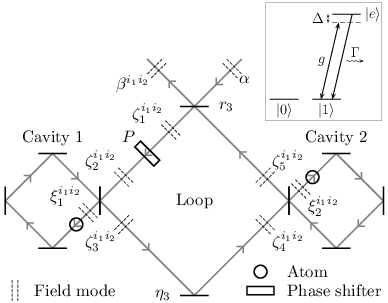
In Sec. II we provide the theoretical framework required to analyze the proposed setup, and we obtain expressions for the field amplitudes, which substantiate the above statements. In Sec. III we derive an equation for the time evolution of the purity of a state restricted to either the odd or the even parity subspace and identify the parameters, which characterize the performance of the proposal. These parameters are evaluated for a nonresonant light-atom interaction in Sec. IV and for a resonant light-atom interaction in Sec. V. We also compute the optimal value of the reflectivity $r_{3}^{2}$ of the input beam splitter and compare the performance of the resonant and the nonresonant interaction. Finally, Sec. VI concludes the paper.

As discussed in Sec. II.1, the probe light does not drive any transitions between the atomic states $|0\rangle$ and $|1\rangle$. On the other hand, the interaction does, in general, lead to entanglement between the atoms and the light field such that the state of the atoms and the state of the light field are correlated. A subsequent detection of the probe field may hence provide information about the state of the atoms, and this will, in general, change the coefficients $c_{i_{1}j_{1}i_{2}j_{2}}(t)$ in Eq. (5). In other words, the back action of the continuous measurement gradually projects the state onto an eigenstate of the measured observable, i.e., onto a state with either even or odd parity. In the ideal case, the measurement is unable to distinguish states within the odd subspace and to distinguish states within the even subspace. A main indication of the quality of the measurement is thus the rate at which a state within the odd subspace or a state within the even subspace decoheres compared to the duration of the measurement, i.e., the time required to distinguish odd parity states from even parity states.

If the atoms are initially in a state of odd parity, the state of the system at time $t$ is given by Eq. (5) with the additional requirements $i_{1}\neq i_{2}$ and $j_{1}\neq j_{2}$. The entanglement between the atoms and the light fields reduces the purity of the atomic state during the measurement, but this purity is regained, when the input field is turned off and the cavity fields decay to the vacuum state. While the rate of nonregainable loss of purity may be slightly different during the initial and final transients, we do not expect anything dramatic to happen, since the transient dynamics does not break the symmetry, which ensures that the odd parity states are indistinguishable in the output field. For a total measurement time $t_{m}$, which is long compared to the transients, we may thus concentrate on the rate of loss of purity in steady state. (This is a matter of $|\alpha|^{2}$ being sufficiently small, since the duration of the transients does not depend on $\alpha$, while $t_{m}^{-1}\propto|\alpha|^{2}$ as we shall find below.)

In the time interval from $t$ to $t+dt$ several interactions take place. The coherent state $|\xi^{10}_{1}\sqrt{\tau_{1}}\rangle$ in cavity 1 interacts with the atom and an average number of $2C_{1}\kappa_{1}dt|\xi^{10}_{1}|^{2}\tau_{1}/(1+D_{1}^{2})$ photons are lost through spontaneous emission. The loss can be modeled as a beam splitter, which transforms $|\xi^{10}_{1}\sqrt{\tau_{1}}\rangle|\textrm{vac}\rangle$ into $|\sqrt{\eta_{\textrm{SE},1}}\xi^{10}_{1}\sqrt{\tau_{1}}\rangle|\sqrt{1-\eta_{\textrm{SE},1}}\xi^{10}_{1}\sqrt{\tau_{1}}\rangle$, where $1-\eta_{\textrm{SE},1}\equiv 2C_{1}\kappa_{1}dt/(1+D_{1}^{2})$, followed by a trace over the last mode. In steady state, $|\sqrt{\eta_{\textrm{SE},1}}\xi^{10}_{1}\sqrt{\tau_{1}}\rangle$ is transformed back into $|\xi^{10}_{1}\sqrt{\tau_{1}}\rangle$ before the next interaction with the atom. The overall transformation is thus

while $c_{1100}$ and $c_{0011}$ are unchanged. Spontaneous emission in cavity 2 leads to a similar transformation, and loss through the lower mirror in Fig. 1 gives rise to a factor $\langle\sqrt{1-\eta_{3}}\zeta_{3}^{01}\sqrt{dt}|\sqrt{1-\eta_{3}}\zeta_{3}^{10}\sqrt{dt}\rangle$ on $c_{1001}$ and the complex conjugate factor on $c_{0110}$. Finally, homodyne detection of the $p$-quadrature of the output field leaves the state unchanged if $\textrm{Im}(\beta^{10})=\textrm{Im}(\beta^{01})$. In fact, if $\beta^{10}=\beta^{01}$, it does not even lead to decoherence if the output field is simply traced out, which is why we do not consider detection inefficiency here.

Collecting the factors for the whole measurement from $0$ to $t_{m}$ and neglecting transients, the final purity of the atomic state after the measurement evaluates to

where $\rho_{\textrm{at}}(t)$ is the density operator of the state of the atoms obtained by tracing out the light fields,

is the rate of spontaneous emission events (i.e., the number of photons emitted spontaneously per unit time) when atom $q$ is in the state $|1\rangle$, and

represents the rate at which it would be possible to distinguish the two states within the odd subspace if the light lost at the lower mirror in Fig. 1 was detected. The interpretation of Eq. (15) follows from the fact that the right hand side is the product of the photon loss rate $\Gamma_{q}g_{q}^{2}/((\Gamma_{q}/2)^{2}+\Delta_{q}^{2})$ from Eq. (4) and the expectation value $|\xi_{q}^{\delta_{1q}\delta_{2q}}|^{2}\tau_{q}$ of the number of photons in cavity $q$, whereas the interpretation of Eq. (16) follows from the result in appendix B. Additional photon losses in cavity 1 and 2 could be taken into account by including a factor of $\sqrt{\eta_{q}}$ in (6) and adding the terms $(1-\eta_{q})|\xi_{q}^{10}-\xi_{q}^{01}|^{2}t_{m}$, $q=1,2$, to the exponent in (14), where $(1-\eta_{q})$ is the fraction of photons lost in cavity $q$ per round trip. In appendix B, we show that the rate of gain of information in homodyne detection is of order the square of the distance between the conditional amplitudes of the output field projected onto the direction of the measured quadrature, and for $\alpha=\alpha^{*}$ and $\textrm{Im}(\beta^{10})=\textrm{Im}(\beta^{01})$, the relevant size of $t_{m}$ is thus

where

If $\textrm{Im}(\beta^{00})=\textrm{Im}(\beta^{11})$, the final purity of a state restricted to the even subspace is likewise

where

and

For $\textrm{Im}(\beta^{00})\neq\textrm{Im}(\beta^{11})$, the two-qubit state is projected onto either $|00\rangle$ or $|11\rangle$ at a rate, which is of order $|\textrm{Im}(\beta^{00})-\textrm{Im}(\beta^{11})|^{2}\sim C^{-2}$, and we need to multiply $|c_{1111}(0)|^{2}$, $|c_{0000}(0)|^{2}$, and $|c_{1010}(0)|^{2}$ by the square of the accumulated weight factors arising due to the measurement.

In the following, we compare the performance of the setup in Fig. 1 with $r_{3}\neq 0$ and an open loop setup with $r_{3}=0$. We first consider a nonresonant light-atom interaction with $D\sim C$ and $C\gg 1$, assuming $D_{1}=D_{2}=D$ and $C_{1}=C_{2}=C$. In this case, the primary effect of the light-atom interaction is a phase shift of the light field, and we apply the approximation $F_{1}^{1}=F_{2}^{1}\approx(D+iC)/(D-iC)\equiv F$ (see Eq. (10)). Furthermore, $F_{1}^{0}=F_{2}^{0}=F^{*}$. Combining $\zeta_{3}^{i_{1}i_{2}}=-iF_{1}^{i_{1}}\zeta_{2}^{i_{1}i_{2}}$, (7), (8), (9), (15), (16), (17), (18), (20), and (21), we then derive

and

The latter four quantities are plotted in Fig. 2, and we note that $\nu_{\textrm{odd},2}^{\textrm{(SE)}}=\eta_{3}\nu_{\textrm{odd},1}^{\textrm{(SE)}}$ and $\nu_{\textrm{even},2}^{\textrm{(SE)}}=\eta_{3}\nu_{\textrm{even},1}^{\textrm{(SE)}}$.

The figure shows that it is possible in the odd subspace to reduce both the rate of spontaneous emission events and the rate of decoherence due to other light field losses relative to the rate of gain of information due to the measurement by choosing a nonzero value of $r_{3}$, but only if $D/C$ is sufficiently close to plus or minus one, which corresponds to the situation of constructive interference in the loop for the even subspace. Note that $\nu_{\textrm{odd},q}^{\textrm{(SE)}}$ and $\nu_{\textrm{odd}}^{\textrm{(L)}}$ depend on $r_{3}$ in the same way, and for a given value of $D/C\in[-\sqrt{3},-1/\sqrt{3}]\cup[1/\sqrt{3},\sqrt{3}]$ and $\eta_{3}=1$, the optimal choice of beam splitter reflectivity is given by

Outside this interval, it is optimal to choose $r_{3}=0$. As far as light field losses in the loop are concerned, the smallest losses occur for $|D|/C=1$, and Fig. 2(a) suggests that this is also a good choice to reduce the total number of spontaneous emission events (the optimal value of $|D|/C$ with respect to loss due to spontaneous emission varies from $\sqrt{2}$ for $\sqrt{\eta_{3}}r_{3}=0$ to $1$ for $\sqrt{\eta_{3}}r_{3}=1$). For $|D|/C\rightarrow 1$, $r_{3,\textrm{opt}}\rightarrow 1$, but since $\sqrt{\eta_{3}}PF_{1}^{1}F_{2}^{1}=+1$ for the even subspace, the results are only valid if $1-r_{3}\gg C^{-1}$. In fact, if $\eta_{3}<1$ or $C$ is not infinite, the curves go to infinity for $r_{3}\rightarrow 1$. This happens because $t_{m}\rightarrow\infty$, which in turn is a consequence of the fact that it is only possible to couple light into the system for $r_{3}=1$ if there is perfect constructive interference within the loop and no loss, and the output field amplitude is hence $i\alpha$ for all states of the qubits if this is not the case. In conclusion, a reasonable strategy is to choose the light-atom detuning such that $|D|/C=1$, and then compute the optimal value of $r_{3}$ from the above expressions if the relative photon loss $1-\eta_{3}$ in the loop is large compared to $C^{-1}$. Otherwise one has to optimize $r_{3}$ under the constraint $|1+r_{3}F_{1}^{1}F_{2}^{1}\sqrt{\eta_{3}}|\gg C^{-1}$. For the even subspace, on the other hand, it is always optimal to choose $r_{3}=0$.

For a resonant light-atom coupling $D=0$ and identical atom and cavity parameters, $F_{1}^{1}=F_{2}^{1}=(1-2C)/(1+2C)\equiv G$ and $F_{1}^{0}=F_{2}^{0}=1$. In this case,

and

while $\nu_{\textrm{odd},2}^{\textrm{(SE)}}=\eta_{3}\nu_{\textrm{odd},1}^{\textrm{(SE)}}$ and $\nu_{\textrm{even},2}^{\textrm{(SE)}}=\eta_{3}G^{2}\nu_{\textrm{even},1}^{\textrm{(SE)}}$. These results are illustrated for $\eta_{3}=1$ in Fig. 3, which shows that the total decoherence in the odd subspace also in this case can be reduced by choosing a nonzero $r_{3}$. For a given value of $C$ and $\eta_{3}$, the minimum appears at $r_{3,\textrm{opt}}=\sqrt{\eta_{3}}G^{2}$, but again one should keep the constraint $|1-r_{3}F_{1}^{1}F_{2}^{1}\sqrt{\eta_{3}}|\gg C^{-1}$ in mind.

Assuming $D=C$ and $C\rightarrow\infty$ for the nonresonant case and $C\rightarrow\infty$ for the resonant case, we observe that the expressions for $t_{m}$ are the same, and the two possibilities are thus equally efficient in distinguishing the even and the odd subspaces. We also note that $\zeta_{1}^{i_{1}i_{2}}$ is the same for the resonant and the nonresonant coupling, leading to the same values for the rate of decoherence due to light field losses in the loop. The rates of spontaneous emission are also the same except for a factor of 2, which arises from the details of the light-atom interaction: For cavities containing an atom in the state $|1\rangle$, the number of photons in the cavity is a factor of $1/(2C^{2})$ smaller in the resonant case compared to the nonresonant case, but the fraction of photons lost per round trip is a factor of $C^{2}$ larger. Finally, the significance of additional photon losses in cavity 1 and 2 is the same for resonant and nonresonant coupling because $|\xi_{q}^{10}-\xi_{q}^{01}|$ is the same and $|\xi_{q}^{11}-\xi_{q}^{00}|$ is the same. The performance is thus roughly the same for a resonant and a nonresonant light-atom interaction.

It is interesting to note that the total number of spontaneous emission events is of order $C^{-1}$, while the contribution to the exponent in (14) from loss at the lower mirror in Fig. 1 is of order $(1-\eta_{3})$, such that the relative importance of the two effects is determined by $C(1-\eta_{3})$. The importance of additional photon losses in cavity 1 or 2 relative to spontaneous emission is likewise given by $C(1-\eta_{q})$. High performance is thus obtained for high cooperativity parameters and low propagation and reflection losses for the light field. On the other hand, Eqs. (23)-(26) and Eqs. (29)-(32) show that the performance is independent of the intensity of the input field as long as Eq. (11) is satisfied. This is the case, because both the rate of gain of information due to the measurement and the photon loss rates scale linearly with $|\alpha|^{2}$. Equation (11) defines an upper limit for $|\alpha|^{2}$, but $|\alpha|^{2}$ should not be chosen too small either in order to limit the time required to carry out the parity measurement.

In conclusion, we have analyzed the performance of a parity measurement on two qubits, each encoded in two ground state levels of a single atom in a cavity. The measurement relies on the phase shift imposed conditionally on a continuous beam of light, which interacts sequentially with the two qubits. We have found that the rate of decoherence within the odd parity subspace due to spontaneous emission and light field losses can be decreased by allowing the probe field to interact several times with the two qubits before it is detected, but the decrease happens at the expense of an increased decoherence rate within the even parity subspace. Finally, we have shown that the performance of the parity measurement is about the same for a resonant and for a nonresonant light-atom interaction if the light-atom detuning is chosen as $|\Delta|=g^{2}/\kappa$, where $g$ is the light-atom coupling strength and $\kappa$ is the decay rate of light in the cavity.

The proposed measurement can, for instance, be used to prepare two qubits in an entangled odd parity state with higher purity. Improvements can also be obtained in quantum error correction if the qubit state is encoded in the odd subspace and errors are corrected continuously such that the even subspace is practically avoided. In case of the three-qubit bit-flip correction code, for instance, one would use the three-qubit states $|010\rangle$ and $|101\rangle$ as the code space and then perform the proposed parity measurement on qubits 1 and 2 and on qubits 2 and 3. This could be done either by switching between the two measurements or by using two different polarizations of the light field, one of which interacts with the qubit state $|1\rangle$ and the other with the qubit state $|0\rangle$. Polarizing beam splitters could then be used to guide the polarization components into the right cavities.

We have presented the proposed structure as a closed loop setup, but we note the similarities with both a coherent feedback loop and a cavity array. The idea of having cavities within cavities and utilizing constructive and destructive interference may be useful in other settings as well.