跳到论文正文
W Papers独立论文阅读器 arXiv:0908.0706 论文正文 计算阅读时间 · 0%
引用这篇论文根据当前论文元数据生成,正式投稿前建议核对。


License: arXiv.org perpetual non-exclusive license
arXiv:0908.0706v3 [quant-ph] 01 Jun 2010

Superqubits

Preprint: Imperial/TP/2009/mjd/2
L. Borsten Email: leron.borsten@imperial.ac.uk Affiliation: Theoretical Physics, Blackett Laboratory, Imperial College London, London SW7 2AZ, United Kingdom    D. Dahanayake Email: duminda.dahanayake@imperial.ac.uk Affiliation: Theoretical Physics, Blackett Laboratory, Imperial College London, London SW7 2AZ, United Kingdom    M. J. Duff Email: m.duff@imperial.ac.uk Affiliation: Theoretical Physics, Blackett Laboratory, Imperial College London, London SW7 2AZ, United Kingdom    W. Rubens Email: william.rubens06@imperial.ac.uk Affiliation: Theoretical Physics, Blackett Laboratory, Imperial College London, London SW7 2AZ, United Kingdom
August 24, 2026
Abstract

We provide a supersymmetric generalization of nn quantum bits by extending the local operations and classical communication entanglement equivalence group [S​U​(2)]n[SU(2)]^{n} to the supergroup [u​O​S​p​(1|2)]n[uOSp(1|2)]^{n} and the stochastic local operations and classical communication equivalence group [S​L​(2,ℂ)]n[SL(2,\mathds{C})]^{n} to the supergroup [O​S​p​(1|2)]n[OSp(1|2)]^{n}. We introduce the appropriate supersymmetric generalizations of the conventional entanglement measures for the cases of n=2n=2 and n=3n=3. In particular, super-Greenberger-Horne-Zeilinger states are characterized by a nonvanishing superhyperdeterminant.

Keywords: 
qubit, entanglement, hyperdeterminant
pacs
11.30.Pb, 03.65.Ud, 03.67.Mn

I Introduction

The question of computable entanglement measures for arbitrary quantum systems is, to a large extent, an open one. However, substantial progress has been made utilizing the paradigms of local operations and classical communication (LOCC) and stochastic local operations and classical communication (SLOCC). For example, 2-qubit and 3-qubit systems both admit concise, but nontrivial, SLOCC classifications which reveal a number of important qualitative features of multipartite entanglement [1, 2, 3, 4, 5, 6]. In particular, 2-qubit Bell states and 3-qubit Greenberger-Horne-Zeilinger (GHZ) states are characterized, respectively, by nonvanishing determinant and hyperdeterminant.

Here we propose a supersymmetric generalization of the qubit, the superqubit. We proceed by extending the nn-qubit SLOCC equivalence group [S​L​(2,ℂ)]n[SL(2,\mathds{C})]^{n} and the LOCC equivalence group [S​U​(2)]n[SU(2)]^{n} to the supergroups [O​S​p​(1|2)]n[OSp(1|2)]^{n} and [u​O​S​p​(1|2)]n[uOSp(1|2)]^{n}, respectively. A single superqubit forms a 3-dimensional representation of O​S​p​(1|2)OSp(1|2) consisting of two commuting “bosonic” components and one anticommuting “fermionic” component. For n=2n=2 and n=3n=3 we introduce the appropriate supersymmetric generalizations of the conventional entanglement measures. In particular, super-Bell and super-GHZ states are characterized, respectively, by nonvanishing superdeterminant (distinct from the Berezinian) and superhyperdeterminant11 1 The present work was in part inspired by the construction of the superhyperdeterminant in [7]..

This mathematical construction seems a very natural one. Moreover, from a physical point of view, it makes contact with various condensed-matter systems. For example, the three-dimensional representation of O​S​p​(1|2)OSp(1|2) is encountered in the supersymmetric tt-JJ model where it describes spinons and holons on a one-dimensional lattice [8, 9, 10, 11, 12]. It also shows up in the quantum Hall effect [13] and Affleck-Kennedy-Lieb-Tasaki models of superconductivity [14].

In order to facilitate the introduction of a super Hilbert space, super LOCC and superqubits in section IV, we first recall some familiar properties of ordinary Hilbert space, LOCC, and qubits in section II. Similarly, in order to discuss the superentanglement of two and three superqubits in section V, we first review the ordinary entanglement of two and three qubits in section III.

II Qubits

II.1 Hilbert space

A complex Hilbert space ℋ\mathcal{H} is equipped with a one-to-one map into its dual space ℋ†\mathcal{H}^{\dagger},

†:ℋ→ℋ†,|ψ⟩↦(|ψ⟩)†:=⟨ψ|\begin{split}{}^{\dagger}:\mathcal{H}&\to\mathcal{H}^{\dagger},\\ \lvert\psi\rangle&\mapsto(\lvert\psi\rangle)^{\dagger}:=\langle\psi\rvert\end{split} (1)

which defines an inner product ⟨ψ|ϕ⟩\langle\psi|\phi\rangle and satisfies the following properties:

  1. 1.

    For all |ψ⟩,|ϕ⟩∈ℋ\lvert\psi\rangle,\lvert\phi\rangle\in\mathcal{H}, and any complex number α\alpha we have,

    (α|ψ⟩)†=⟨ψ|α∗,(|ψ⟩+|ϕ⟩)†=⟨ψ|+⟨ϕ|.\begin{split}(\alpha\lvert\psi\rangle)^{\dagger}&=\langle\psi\rvert\alpha^{*},\\ (\lvert\psi\rangle+\lvert\phi\rangle)^{\dagger}&=\langle\psi\rvert+\langle\phi\rvert.\end{split} (2)
  2. 2.

    For all |ψ⟩,|ϕ⟩∈ℋ\lvert\psi\rangle,\lvert\phi\rangle\in\mathcal{H},

    ⟨ψ|ϕ⟩∗=⟨ϕ|ψ⟩.\langle\psi|\phi\rangle^{*}=\langle\phi|\psi\rangle. (3)
  3. 3.

    For all |ψ⟩∈ℋ\lvert\psi\rangle\in\mathcal{H},

    ⟨ψ|ψ⟩≥0\langle\psi|\psi\rangle\geq 0 (4)

    with equality holding if and only if |ψ⟩\lvert\psi\rangle is the null vector.

In particular a qubit lives in the two-dimensional complex Hilbert space ℂ2\mathds{C}^{2}. An arbitrary nn-qubit system is then simply a vector in the nn-fold tensor product Hilbert space ℂ2⊗⋯⊗ℂ2=[ℂ2]n\mathds{C}^{2}\otimes\dotsb\otimes\mathds{C}^{2}=[\mathds{C}^{2}]^{n}.

II.2 LOCC and SLOCC

Two states are said to be LOCC equivalent if and only if they may be transformed into one another with certainty using LOCC protocols. Reviews of the LOCC paradigm and entanglement measures may be found in [15, 16]. It is well known that two states of a composite system are LOCC equivalent if and only if they are related by the group of local unitaries (which we will refer to as the LOCC equivalence group), unitary transformations that factorize into separate transformations on the component parts [17]. In the case of nn qubits the group of local unitaries is given (up to a global phase) by [S​U​(2)]n[SU(2)]^{n}.

Similarly, two quantum states are said to be SLOCC equivalent if and only if they may be transformed into one another with some nonvanishing probability using LOCC operations [17, 2]. The set of SLOCC transformations relating equivalent states forms a group (which we will refer to as the SLOCC equivalence group). For nn qubits the SLOCC equivalence group is given (up to a global complex factor) by the nn-fold tensor product, [S​L​(2,ℂ)]n[SL(2,\mathds{C})]^{n}, one factor for each qubit [2]. Note, the LOCC equivalence group forms a compact subgroup of the larger SLOCC equivalence group.

The Lie algebra 𝔰​𝔩​(2)\mathfrak{sl}(2) may be conveniently summarized as

[PA1​A2,PA3​A4]=2​ε(A1​(A3CLOSECLOSE​POPENOPENA4)​A2)\left[P_{A_{1}A_{2}},P_{A_{3}A_{4}}\right]=2\varepsilon_{(A_{1}(A_{3}}P_{A_{4})A_{2})} (5)

where A=0,1A=0,1, and throughout this paper we use “strength one” (anti)symmetrization, so that

X(A1​A2)≡12​(XA1​A2+XA2​A1).X_{(A_{1}A_{2})}\equiv\tfrac{1}{2}(X_{A_{1}A_{2}}+X_{A_{2}A_{1}}). (6)

We permit the indices to be raised/lowered by the S​L​(2,ℂ)SL(2,\mathds{C})–invariant epsilon tensors according to the rules:

VA1\displaystyle V_{A_{1}} =εA1​A2​VA2\displaystyle=\varepsilon_{A_{1}A_{2}}V^{A_{2}} VA1\displaystyle V^{A_{1}} =εA1​A2​VA2,\displaystyle=\varepsilon^{A_{1}A_{2}}V_{A_{2}}, (7)

where we adopt the following conventions

εA1​A2=−εA1​A2,εA1​A2​εA2​A3=δA1A3.\varepsilon_{A_{1}A_{2}}=-\varepsilon^{A_{1}A_{2}},\quad\varepsilon_{A_{1}A_{2}}\varepsilon^{A_{2}A_{3}}=\delta_{A_{1}}^{A_{3}}. (8)

Consequently,

UA​VA=−UA​VA.U^{A}V_{A}=-U_{A}V^{A}. (9)

The compact subalgebra 𝔰​𝔲​(2)\mathfrak{su}(2) is given by

𝔰​𝔲​(2):={X∈𝔰​𝔩​(2)|X†=−X}.\mathfrak{su}(2):=\{X\in\mathfrak{sl}(2)|X^{\dagger}=-X\}. (10)

An arbitrary element X∈𝔰​𝔲​(2)X\in\mathfrak{su}(2) may be written as

X=ξi​Ai,X=\xi_{i}A_{i}, (11)

where ξi∈ℝ\xi_{i}\in\mathds{R} and

A1=i2​(P00−P11),A2=12​(P00+P11),A3=i​P01,Ai†=−Ai.\begin{gathered}A_{1}=\tfrac{i}{2}(P_{00}-P_{11}),\\ A_{2}=\tfrac{1}{2}(P_{00}+P_{11}),\\ A_{3}=iP_{01},\\ A_{i}^{{\dagger}}=-A_{i}.\end{gathered} (12)

II.3 One qubit

The one-qubit system (Alice) is described by the state

|Ψ⟩=aA|A⟩,\lvert\Psi\rangle=a_{A}\lvert A\rangle, (13)

and the Hilbert space has dimension 22. The SLOCC equivalence group is S​L​(2,ℂ)ASL(2,\mathds{C})_{A}, under which aAa_{A} transforms as a 2.

The norm squared ⟨Ψ|Ψ⟩\langle\Psi|\Psi\rangle is given by

⟨Ψ|Ψ⟩=δA1​A2​aA1∗​aA2\langle\Psi|\Psi\rangle=\delta^{A_{1}A_{2}}a_{A_{1}}^{*}a_{A_{2}} (14)

and is invariant under S​U​(2)ASU(2)_{A}. The one-qubit density matrix is given by

ρ:=|Ψ⟩⟨Ψ|=aA1aA2∗|A1⟩⟨A2|.\begin{split}\rho&:=\lvert\Psi\rangle\!\langle\Psi\rvert\\ &=a_{A_{1}}a_{A_{2}}^{*}\lvert{A_{1}}\rangle\!\langle{A_{2}}\rvert.\end{split} (15)

The norm squared is then given by

⟨Ψ|Ψ⟩=tr⁡(ρ).\langle\Psi|\Psi\rangle=\tr(\rho). (16)

Unnormalized pure state density matrices satisfy

ρ2=tr⁡(ρ)​ρ.\rho^{2}=\tr(\rho)\rho. (17)

II.4 Two qubits

The two-qubit system (Alice and Bob) is described by the state

|Ψ⟩=aA​B|AB⟩,\lvert\Psi\rangle=a_{AB}\lvert AB\rangle, (18)

and the Hilbert space has dimension 22=42^{2}=4. The SLOCC equivalence group is S​L​(2,ℂ)A×S​L​(2,ℂ)BSL(2,\mathds{C})_{A}\times SL(2,\mathds{C})_{B} under which aA​Ba_{AB} transforms as a (𝟐,𝟐)\mathbf{(2,2)}.

The norm squared ⟨Ψ|Ψ⟩\langle\Psi|\Psi\rangle is given by

⟨Ψ|Ψ⟩=δA1​A2​δB1​B2​aA1​B1∗​aA2​B2.\langle\Psi|\Psi\rangle=\delta^{A_{1}A_{2}}\delta^{B_{1}B_{2}}a_{A_{1}B_{1}}^{*}a_{A_{2}B_{2}}. (19)

and is invariant under S​U​(2)A×S​U​(2)BSU(2)_{A}\times SU(2)_{B}. The two-qubit density matrix is given by

ρ:=|Ψ⟩⟨Ψ|=aA1​B1aA2​B2∗|A1B1⟩⟨A2B2|.\begin{split}\rho&:=\lvert\Psi\rangle\!\langle\Psi\rvert\\ &=a_{A_{1}B_{1}}a_{A_{2}B_{2}}^{*}\lvert{A_{1}B_{1}}\rangle\!\langle{A_{2}B_{2}}\rvert.\end{split} (20)

The reduced density matrices are defined using the partial trace

ρA=trB|Ψ⟩⟨Ψ|,ρB=trA|Ψ⟩⟨Ψ|,\begin{split}\rho_{A}=\tr_{B}\lvert\Psi\rangle\langle\Psi\rvert,\\ \rho_{B}=\tr_{A}\lvert\Psi\rangle\langle\Psi\rvert,\\ \end{split} (21)

or

(ρA)A1​A2=δB1​B2​aA1​B1​aA2​B2∗,(ρB)B1​B2=δA1​A2​aA1​B1​aA2​B2∗.\begin{split}(\rho_{A})_{A_{1}A_{2}}&=\delta^{B_{1}B_{2}}a_{A_{1}B_{1}}a^{*}_{A_{2}B_{2}},\\ (\rho_{B})_{B_{1}B_{2}}&=\delta^{A_{1}A_{2}}a_{A_{1}B_{1}}a^{*}_{A_{2}B_{2}}.\end{split} (22)

II.5 Three qubits

The three-qubit system (Alice, Bob, Charlie) is described by the state

|Ψ⟩=aA​B​C|ABC⟩,\lvert\Psi\rangle=a_{ABC}\lvert ABC\rangle, (23)

and the Hilbert space has dimension 23=82^{3}=8. The SLOCC equivalence group is S​L​(2,ℂ)A×S​L​(2,ℂ)B×S​L​(2,ℂ)CSL(2,\mathds{C})_{A}\times SL(2,\mathds{C})_{B}\times SL(2,\mathds{C})_{C} under which aA​B​Ca_{ABC} transforms as a (𝟐,𝟐,𝟐)\mathbf{(2,2,2)}.

The norm squared ⟨Ψ|Ψ⟩\langle\Psi|\Psi\rangle is given by

⟨Ψ|Ψ⟩=δA1​A2​δB1​B2​δC1​C2​aA1​B1​C1∗​aA2​B2​C2\langle\Psi|\Psi\rangle=\delta^{A_{1}A_{2}}\delta^{B_{1}B_{2}}\delta^{C_{1}C_{2}}a_{A_{1}B_{1}C_{1}}^{*}a_{A_{2}B_{2}C_{2}} (24)

and is invariant under S​U​(2)A×S​U​(2)B×S​U​(2)CSU(2)_{A}\times SU(2)_{B}\times SU(2)_{C}. The three-qubit density matrix is given by

ρ:=|Ψ⟩⟨Ψ|=aA1​B1​C1aA2​B2​C2∗|A1B1C1⟩⟨A2B2C2|.\begin{split}\rho&:=\lvert\Psi\rangle\!\langle\Psi\rvert\\ &=a_{A_{1}B_{1}C_{1}}a_{A_{2}B_{2}C_{2}}^{*}\lvert{A_{1}B_{1}C_{1}}\rangle\!\langle{A_{2}B_{2}C_{2}}\rvert.\end{split} (25)

The singly reduced density matrices are defined using the partial trace

ρA​B=trC|Ψ⟩⟨Ψ|,ρB​C=trA|Ψ⟩⟨Ψ|,ρC​A=trB|Ψ⟩⟨Ψ|,\begin{split}\rho_{AB}&=\tr_{C}\lvert\Psi\rangle\langle\Psi\rvert,\\ \rho_{BC}&=\tr_{A}\lvert\Psi\rangle\langle\Psi\rvert,\\ \rho_{CA}&=\tr_{B}\lvert\Psi\rangle\langle\Psi\rvert,\end{split} (26)

or

(ρA​B)A1​A2​B1​B2=δC1​C2​aA1​B1​C1​aA2​B2​C2∗,(ρB​C)B1​B2​C1​C2=δA1​A2​aA1​B1​C1​aA2​B2​C2∗,(ρC​A)C1​C2​A1​A2=δB1​B2​aA1​B1​C1​aA2​B2​C2∗.\begin{split}(\rho_{AB})_{A_{1}A_{2}B_{1}B_{2}}&=\delta^{C_{1}C_{2}}a_{A_{1}B_{1}C_{1}}a^{*}_{A_{2}B_{2}C_{2}},\\ (\rho_{BC})_{B_{1}B_{2}C_{1}C_{2}}&=\delta^{A_{1}A_{2}}a_{A_{1}B_{1}C_{1}}a^{*}_{A_{2}B_{2}C_{2}},\\ (\rho_{CA})_{C_{1}C_{2}A_{1}A_{2}}&=\delta^{B_{1}B_{2}}a_{A_{1}B_{1}C_{1}}a^{*}_{A_{2}B_{2}C_{2}}.\end{split} (27)

The doubly reduced density matrices are defined using the partial traces

ρA=trB​C|Ψ⟩⟨Ψ|,ρB=trC​A|Ψ⟩⟨Ψ|,ρC=trA​B|Ψ⟩⟨Ψ|,\begin{split}\rho_{A}&=\tr_{BC}\lvert\Psi\rangle\langle\Psi\rvert,\\ \rho_{B}&=\tr_{CA}\lvert\Psi\rangle\langle\Psi\rvert,\\ \rho_{C}&=\tr_{AB}\lvert\Psi\rangle\langle\Psi\rvert,\end{split} (28)

or

(ρA)A1​A2=δB1​B2​δC1​C2​aA1​B1​C1​aA2​B2​C2∗,(ρB)B1​B2=δC1​C2​δA1​A2​aA1​B1​C1​aA2​B2​C2∗,(ρC)C1​C2=δA1​A2​δB1​B2​aA1​B1​C1​aA2​B2​C2∗.\begin{split}(\rho_{A})_{A_{1}A_{2}}&=\delta^{B_{1}B_{2}}\delta^{C_{1}C_{2}}a_{A_{1}B_{1}C_{1}}a^{*}_{A_{2}B_{2}C_{2}},\\ (\rho_{B})_{B_{1}B_{2}}&=\delta^{C_{1}C_{2}}\delta^{A_{1}A_{2}}a_{A_{1}B_{1}C_{1}}a^{*}_{A_{2}B_{2}C_{2}},\\ (\rho_{C})_{C_{1}C_{2}}&=\delta^{A_{1}A_{2}}\delta^{B_{1}B_{2}}a_{A_{1}B_{1}C_{1}}a^{*}_{A_{2}B_{2}C_{2}}.\end{split} (29)

III Entanglement

III.1 Two qubits

For two qubits there are only two distinct SLOCC entanglement classes - two qubits are either entangled or not. The two classes are distinguished by the SLOCC invariant, detaA​B\det a_{AB}. For separable states detaA​B=0\det a_{AB}=0, while it is nonzero for any entangled state.

There are two independent [S​U​(2)]2[SU(2)]^{2} invariants, the norm ⟨Ψ|Ψ⟩1/2\langle\Psi|\Psi\rangle^{1/2} and the 2-tangle τA​B\tau_{AB} [18, 1],

τA​B=4​detρA=4​detρB=4​|detaA​B|2.\tau_{AB}=4\det\rho_{A}=4\det\rho_{B}=4|\det a_{AB}|^{2}. (30)

The 2-tangle is maximized, τA​B=1\tau_{AB}=1, by the Bell state:

|Ψ⟩Bell=12(|00⟩+|11⟩).\lvert\Psi\rangle_{\textrm{Bell}}=\tfrac{1}{\sqrt{2}}(\lvert 00\rangle+\lvert 11\rangle). (31)

III.2 Three qubits

For three qubits there are six distinct SLOCC entanglement classes [2, 4, 5, 6]. These classes and their representative states are summarized as follows:

Separable

Zero entanglement orbit for completely factorisable product states,

A-B-C:|000⟩.A\text{-}B\text{-}C:\quad\lvert 000\rangle. (32)
Biseparable

Three classes of bipartite entanglement

A-BC:|010⟩+|001⟩,B-CA:|100⟩+|001⟩,C-AB:|010⟩+|100⟩.\begin{split}A\text{-}BC:\quad\lvert 010\rangle+\lvert 001\rangle,\\ B\text{-}CA:\quad\lvert 100\rangle+\lvert 001\rangle,\\ C\text{-}AB:\quad\lvert 010\rangle+\lvert 100\rangle.\end{split} (33)
W

Three-way entangled states that do not maximally violate Bell-type inequalities in the same way as the GHZ class discussed below. However, they are robust in the sense that tracing out a subsystem generically results in a bipartite mixed state that is maximally entangled under a number of criteria [2],

W:|100⟩+|010⟩+|001⟩.\text{W}:\quad\lvert 100\rangle+\lvert 010\rangle+\lvert 001\rangle. (34)
GHZ

Genuinely tripartite entangled Greenberger-Horne-Zeilinger [19] states. These maximally violate Bell’s inequalities but, in contrast to class W, are fragile under the tracing out of a subsystem since the resultant state is completely unentangled,

GHZ:|000⟩+|111⟩.\text{GHZ}:\quad\lvert 000\rangle+\lvert 111\rangle. (35)

The six classes may be distinguished either by appealing to simple arguments concerning the conservation of reduced density matrix ranks as in [2] or by considering the vanishing or not of five algebraically independent covariants/invariants as in [6]. For our purposes it is more convenient to follow the latter approach as it better facilitates our supersymmetric extension. The five covariants/invariants are given as follows:

  1. 1.

    Three covariants

    (γA)A1​A2=aA1​​B​C​aA2​B​C,(γB)B1​B2=a​B1​A​​C​aA​B2​C,(γC)C1​C2=a​C1A​B​​aA​B​C2,\displaystyle\begin{split}(\gamma^{A})_{A_{1}A_{2}}&=a^{{\mathchoice{\makebox[8.96391pt][c]{$\displaystyle$}}{\makebox[8.96391pt][c]{$\textstyle$}}{\makebox[5.925pt][c]{$\scriptstyle$}}{\makebox[4.875pt][c]{$\scriptscriptstyle$}}{BC}}}_{{{A_{1}}\mathchoice{\makebox[12.60898pt][c]{$\displaystyle$}}{\makebox[12.60898pt][c]{$\textstyle$}}{\makebox[7.81512pt][c]{$\scriptstyle$}}{\makebox[5.58223pt][c]{$\scriptscriptstyle$}}}}a_{A_{2}BC},\\ (\gamma^{B})_{B_{1}B_{2}}&=a^{{{A}\mathchoice{\makebox[9.333pt][c]{$\displaystyle$}}{\makebox[9.333pt][c]{$\textstyle$}}{\makebox[6.21252pt][c]{$\scriptstyle$}}{\makebox[5.08037pt][c]{$\scriptscriptstyle$}}{C}}}_{{\mathchoice{\makebox[6.01392pt][c]{$\displaystyle$}}{\makebox[6.01392pt][c]{$\textstyle$}}{\makebox[3.675pt][c]{$\scriptstyle$}}{\makebox[2.625pt][c]{$\scriptscriptstyle$}}{B_{1}}\mathchoice{\makebox[6.22598pt][c]{$\displaystyle$}}{\makebox[6.22598pt][c]{$\textstyle$}}{\makebox[3.8526pt][c]{$\scriptstyle$}}{\makebox[2.75186pt][c]{$\scriptscriptstyle$}}}}a_{AB_{2}C},\\ (\gamma^{C})_{C_{1}C_{2}}&=a^{{{AB}\mathchoice{\makebox[9.17598pt][c]{$\displaystyle$}}{\makebox[9.17598pt][c]{$\textstyle$}}{\makebox[6.1026pt][c]{$\scriptstyle$}}{\makebox[5.00186pt][c]{$\scriptscriptstyle$}}}}_{{\mathchoice{\makebox[12.39691pt][c]{$\displaystyle$}}{\makebox[12.39691pt][c]{$\textstyle$}}{\makebox[7.63753pt][c]{$\scriptstyle$}}{\makebox[5.45537pt][c]{$\scriptscriptstyle$}}{C_{1}}}}a_{ABC_{2}},\end{split} (36)

    transforming, respectively, as a (𝟑,𝟏,𝟏)\mathbf{(3,1,1)}, (𝟏,𝟑,𝟏)\mathbf{(1,3,1)}, and (𝟏,𝟏,𝟑)\mathbf{(1,1,3)} under S​LA​(2,ℂ)×S​LB​(2,ℂ)×S​LC​(2,ℂ)SL_{A}(2,\mathds{C})\times SL_{B}(2,\mathds{C})\times SL_{C}(2,\mathds{C}).

  2. 2.

    One covariant TA​B​CT_{ABC} transforming as a (𝟐,𝟐,𝟐)\bf{(2,2,2)} under [S​L​(2,ℂ)]3[SL(2,\mathds{C})]^{3}, which may be written in one of three equivalent forms

    TA​B​C=(γA)A​A′​a​B​CA′​TA​B​C=(γB)B​B′​aA​​C​B′​TA​B​C=(γC)C​C′​aA​B​​C′.\begin{split}T_{ABC}&=(\gamma^{A})_{AA^{\prime}}a^{{{A^{\prime}}\mathchoice{\makebox[12.60898pt][c]{$\displaystyle$}}{\makebox[12.60898pt][c]{$\textstyle$}}{\makebox[7.81512pt][c]{$\scriptstyle$}}{\makebox[5.58223pt][c]{$\scriptscriptstyle$}}}}_{{\mathchoice{\makebox[7.8614pt][c]{$\displaystyle$}}{\makebox[7.8614pt][c]{$\textstyle$}}{\makebox[5.1375pt][c]{$\scriptstyle$}}{\makebox[4.0875pt][c]{$\scriptscriptstyle$}}{BC}}}\\ T_{ABC}&=(\gamma^{B})_{BB^{\prime}}a^{{\mathchoice{\makebox[6.01392pt][c]{$\displaystyle$}}{\makebox[6.01392pt][c]{$\textstyle$}}{\makebox[3.675pt][c]{$\scriptstyle$}}{\makebox[2.625pt][c]{$\scriptscriptstyle$}}{B^{\prime}}\mathchoice{\makebox[6.22598pt][c]{$\displaystyle$}}{\makebox[6.22598pt][c]{$\textstyle$}}{\makebox[3.8526pt][c]{$\scriptstyle$}}{\makebox[2.75186pt][c]{$\scriptscriptstyle$}}}}_{{{A}\mathchoice{\makebox[8.23048pt][c]{$\displaystyle$}}{\makebox[8.23048pt][c]{$\textstyle$}}{\makebox[5.42502pt][c]{$\scriptstyle$}}{\makebox[4.29286pt][c]{$\scriptscriptstyle$}}{C}}}\\ T_{ABC}&=(\gamma^{C})_{CC^{\prime}}a^{{\mathchoice{\makebox[12.39691pt][c]{$\displaystyle$}}{\makebox[12.39691pt][c]{$\textstyle$}}{\makebox[7.63753pt][c]{$\scriptstyle$}}{\makebox[5.45537pt][c]{$\scriptscriptstyle$}}{C^{\prime}}}}_{{{AB}\mathchoice{\makebox[8.07347pt][c]{$\displaystyle$}}{\makebox[8.07347pt][c]{$\textstyle$}}{\makebox[5.3151pt][c]{$\scriptstyle$}}{\makebox[4.21436pt][c]{$\scriptscriptstyle$}}}}.\end{split} (37)
  3. 3.

    Cayley’s hyperdeterminant Det⁡aA​B​C\Det a_{ABC} [20, 4, 5], the unique quartic [S​L​(2,ℂ)]3[SL(2,\mathds{C})]^{3} invariant, where

    DetaA​B​C=−detγA=−detγB=−detγC.\Det a_{ABC}=-\det\gamma^{A}=-\det\gamma^{B}=-\det\gamma^{C}. (38)

The entanglement classification as determined by these covariants/invariants is summarized in Table 1.

Table 1: The entanglement classification of three qubits.
Class Vanishing Nonvanishing
AA-BB-CC γA,γB,γC\gamma^{A},\gamma^{B},\gamma^{C} aA​B​Ca_{ABC}
AA-B​CBC γB,γC\gamma^{B},\gamma^{C} γA\gamma^{A}
BB-C​ACA γA,γC\gamma^{A},\gamma^{C} γB\gamma^{B}
CC-A​BAB γA,γB\gamma^{A},\gamma^{B} γC\gamma^{C}
W Det⁡aA​B​C\Det a_{ABC} TA​B​CT_{ABC}
GHZ ⋯\cdots Det⁡aA​B​C\Det a_{ABC}

There are six independent [S​U​(2)]3[SU(2)]^{3} pure state invariants [21]: the norm, the three local entropies 4​detρA4\det\rho_{A}, 4​detρB4\det\rho_{B}, 4​detρC4\det\rho_{C}, the Kempe invariant [22], and finally the all important 3-tangle τA​B​C\tau_{ABC} [1],

τA​B​C=4​|Det⁡aA​B​C|.\tau_{ABC}=4|\Det a_{ABC}|. (39)

The 3-tangle is maximized, τA​B​C=1\tau_{ABC}=1, by the GHZ state:

|Ψ⟩GHZ=12(|000⟩+|111⟩).\lvert\Psi\rangle_{\textrm{GHZ}}=\tfrac{1}{\sqrt{2}}(\lvert 000\rangle+\lvert 111\rangle). (40)

IV Superqubits

IV.1 Super Hilbert space and u​O​S​p​(1|2)uOSp(1|2)

IV.1.1 The dual space

With one important difference, explained below, our definition of a super Hilbert space follows that of DeWitt [23]. We define a super Hilbert space to be a supervector space ℋ\mathcal{H} equipped with an injection to its dual space ℋ‡\mathcal{H}^{\ddagger},

‡:ℋ→ℋ‡,|ψ⟩↦(|ψ⟩)‡:=⟨ψ|.\begin{split}{}^{\ddagger}:\mathcal{H}&\to\mathcal{H}^{\ddagger},\\ \lvert\psi\rangle&\mapsto(\lvert\psi\rangle)^{\ddagger}:=\langle\psi\rvert.\end{split} (41)

Details of even and odd Grassmann numbers and supervectors may be found in Appendix A. A basis in which all basis vectors are pure even or odd is said to be pure. Such a basis may always be found [23].

The map ‡:ℋ→ℋ‡{}^{\ddagger}:\mathcal{H}\to\mathcal{H}^{\ddagger} defines an inner product ⟨ψ|ϕ⟩\langle\psi|\phi\rangle and satisfies the following axioms:

  1. 1.

    ‡ sends pure bosonic (fermionic) supervectors in ℋ\mathcal{H} into bosonic (fermionic) supervectors in ℋ‡\mathcal{H}^{\ddagger}.

  2. 2.

    ‡ is linear

    (|ψ⟩+|ϕ⟩)‡=⟨ψ|+⟨ϕ|.(\lvert\psi\rangle+\lvert\phi\rangle)^{\ddagger}=\langle\psi\rvert+\langle\phi\rvert. (42)
  3. 3.

    For pure even/odd α\alpha and |ψ⟩\lvert\psi\rangle

    (|ψ⟩α)‡=(−)α​ψα#⟨ψ|(\lvert\psi\rangle\alpha)^{\ddagger}=(-)^{\alpha\psi}\alpha^{\#}\langle\psi\rvert (43)

    and

    (α⟨ψ|)‡=(−)ψ+α​ψ|ψ⟩α#,(\alpha\langle\psi\rvert)^{\ddagger}=(-)^{\psi+\alpha\psi}\lvert\psi\rangle\alpha^{\#}, (44)

    where # is the superstar introduced in Appendix A. In particular,

    |ψ⟩‡⁣‡=(−)ψ|ψ⟩.\lvert\psi\rangle^{{\ddagger}{\ddagger}}=(-)^{\psi}\lvert\psi\rangle. (45)

    Note, an α\alpha (or ψ\psi and the like) appearing in the exponent of (−)(-) is shorthand for its grade, deg⁡(α)\deg(\alpha), which takes the value 00 or 11 according to whether α\alpha is even or odd. The impure case follows from the linearity of ‡.

In a pure even/odd orthonormal basis {|i⟩}\{\lvert i\rangle\} we adopt the following convention:

|ψ⟩=|i⟩ψi\lvert\psi\rangle=\lvert i\rangle\psi_{i} (46)

so that for pure even/odd ψ\psi (43) and (44) imply

(|i⟩ψi)‡=(−)ψi​iψi#⟨i|=(−)i+i​ψψi#⟨i|((−)i+i​ψψi#⟨i|)‡=(−)ψ|i⟩ψi\begin{split}(\lvert i\rangle\psi_{i})^{\ddagger}&=(-)^{\psi_{i}i}\psi_{i}^{\#}\langle i\rvert=(-)^{i+i\psi}\psi_{i}^{\#}\langle i\rvert\\ ((-)^{i+i\psi}\psi_{i}^{\#}\langle i\rvert)^{\ddagger}&=(-)^{\psi}\lvert i\rangle\psi_{i}\end{split} (47)

where we have used deg⁡(ψi)=deg⁡(i)+deg⁡(ψ)\deg(\psi_{i})=\deg(i)+\deg(\psi). This is consistent with (150).

IV.1.2 Inner product

For all pure even/odd |ψ⟩,|ϕ⟩∈ℋ\lvert\psi\rangle,\lvert\phi\rangle\in\mathcal{H} the inner product ⟨ψ|ϕ⟩\langle\psi|\phi\rangle satisfies

⟨ψ|ϕ⟩#=(−)ψ+ψ​ϕ​⟨ϕ|ψ⟩.\langle\psi|\phi\rangle^{\#}=(-)^{\psi+\psi\phi}\langle\phi|\psi\rangle. (48)

Consequently,

⟨ψ|ϕ⟩#​#=(−)ψ+ϕ​⟨ϕ|ψ⟩,\langle\psi|\phi\rangle^{\#\#}=(-)^{\psi+\phi}\langle\phi|\psi\rangle, (49)

as would be expected of a pure even/odd Grassmann number since deg⁡(⟨ϕ|ψ⟩)=deg⁡(ψ)+deg⁡(ϕ)\deg(\langle\phi|\psi\rangle)=\deg(\psi)+\deg(\phi). In a pure even/odd orthonormal basis we find

⟨ϕ|ψ⟩=(−)i+i​ϕ​ϕi#​ψi.\langle\phi|\psi\rangle=(-)^{i+i\phi}\phi_{i}^{\#}\psi_{i}. (50)

In using the superstar we depart from the formalism presented in [23], which uses the ordinary star. A comparison of the star and superstar may be found in Appendix A . The use of the superstar anticipates the implementation of u​O​S​p​(1|2)uOSp(1|2) as the compact subgroup of O​S​p​(1|2)OSp(1|2) as will be explained in subsection IV.2.

IV.1.3 Linear superoperators and the superadjoint

A linear superoperator A:ℋ→ℋA:\mathcal{H}\rightarrow\mathcal{H} is required to satisfy the following properties:

  1. 1.

    A(|ψ⟩+|ϕ⟩)=A|ψ⟩+A|ϕ⟩,A(\lvert\psi\rangle+\lvert\phi\rangle)=A\lvert\psi\rangle+A\lvert\phi\rangle,

  2. 2.

    A(|ψ⟩α)=(A|ψ⟩)α.A(\lvert\psi\rangle\alpha)=(A\lvert\psi\rangle)\alpha.

Linear superoperators may be combined using

  1. 1.

    (A+B)|ψ⟩=A|ψ⟩+B|ψ⟩,(A+B)\lvert\psi\rangle=A\lvert\psi\rangle+B\lvert\psi\rangle,

  2. 2.

    (AB)|ψ⟩=A(B|ψ⟩).(AB)\lvert\psi\rangle=A(B\lvert\psi\rangle).

A linear superoperator is said to be pure even (odd) if it takes pure even supervectors into pure even (odd) supervectors and pure odd supervectors into pure odd (even) supervectors.

The superadjoint of a pure even/odd linear superoperator is defined through

(A|ϕ⟩)‡=(−)ϕ​A⟨ϕ|A‡.(A\lvert\phi\rangle)^{\ddagger}=(-)^{\phi A}\langle\phi\rvert A^{\ddagger}. (51)

This is in fact equivalent to

⟨ϕ|A‡|ψ⟩=(−)ψ+ϕ​ψ+(ϕ+ψ)​A⟨ψ|A|ϕ⟩#,\langle\phi\rvert A^{\ddagger}\lvert\psi\rangle=(-)^{\psi+\phi\psi+(\phi+\psi)A}\langle\psi\rvert A\lvert\phi\rangle^{\#}, (52)

which is the natural supersymmetric generalization of the conventional definition of the adjoint. This equivalence may be established by simply inserting the identity operator, 𝟙=|i⟩⟨i|\mathds{1}=\lvert i\rangle\!\langle i\rvert, in (51),

(|i⟩⟨i|A|ϕ⟩)‡=(−)ϕ​A⟨ϕ|A‡|i⟩⟨i|⇒(−)i⁡(i+A+ϕ)⟨i|A|ϕ⟩#⟨i|=(−)ϕ​A⟨ϕ|A‡|i⟩⟨i|⇒(−)i+i​ϕ+(i+ϕ)​A⟨i|A|ϕ⟩#=⟨ϕ|A‡|i⟩⇒∑i(−)i+i​ϕ+(i+ϕ)​A⟨i|A|ϕ⟩#ψi=∑i⟨ϕ|A‡|i⟩ψi⇒∑i(−)i+i​ϕ+(i+ϕ)​A+ψi​(i+A+ϕ)+ψi(ψi#⟨i|A|ϕ⟩)#=∑i⟨ϕ|A‡|i⟩ψi⇒(−)ψ+ϕ​ψ+(ψ+ϕ)​A⟨ψ|A|ϕ⟩#=⟨ϕ|A‡|ψ⟩,\begin{array}[]{cr@{}l@{\ =\ }r@{}l}&(\lvert i\rangle\!\langle i\rvert&A\lvert\phi\rangle)^{\ddagger}&(-)^{\phi A}\langle\phi\rvert&A^{\ddagger}\lvert i\rangle\!\langle i\rvert\\ \Rightarrow&(-)^{i(i+A+\phi)}\langle i\rvert&A\lvert\phi\rangle^{\#}\langle i\rvert&(-)^{\phi A}\langle\phi\rvert&A^{\ddagger}\lvert i\rangle\!\langle i\rvert\\ \Rightarrow&(-)^{i+i\phi+(i+\phi)A}\langle i\rvert&A\lvert\phi\rangle^{\#}&\langle\phi\rvert&A^{\ddagger}\lvert i\rangle\\ \Rightarrow&\sum_{i}(-)^{i+i\phi+(i+\phi)A}\langle i\rvert&A\lvert\phi\rangle^{\#}\psi_{i}&\sum_{i}\langle\phi\rvert&A^{\ddagger}\lvert i\rangle\psi_{i}\\ \Rightarrow&\sum_{i}(-)^{i+i\phi+(i+\phi)A+\psi_{i}(i+A+\phi)+\psi_{i}}(\psi_{i}^{\#}\langle i\rvert&A\lvert\phi\rangle)^{\#}&\sum_{i}\langle\phi\rvert&A^{\ddagger}\lvert i\rangle\psi_{i}\\ \Rightarrow&(-)^{\psi+\phi\psi+(\psi+\phi)A}\langle\psi\rvert&A\lvert\phi\rangle^{\#}&\langle\phi\rvert&A^{\ddagger}\lvert\psi\rangle,\end{array} (53)

where we have defined |ψ⟩=|i⟩ψi\lvert\psi\rangle=\lvert i\rangle\psi_{i} and used deg⁡(ψ)=deg⁡(ψi)+deg⁡(i)\deg(\psi)=\deg(\psi_{i})+\deg(i). The converse implication follows from a similar treatment, which we omit. From (52) we also have

(⟨ϕ|A)‡=(−)ϕ+ϕ​AA‡|ϕ⟩.(\langle\phi\rvert A)^{\ddagger}=(-)^{\phi+\phi A}A^{\ddagger}\lvert\phi\rangle. (54)

Moreover,

A‡⁣‡=(−)A​A,A^{{\ddagger}{\ddagger}}=(-)^{A}A, (55)

which is consistent with the properties of supermatrices and the supermatrix superadjoint given in Appendix A.

In a pure even/odd orthonormal basis the supermatrix representation of a linear operator AA is given by

Ai​j:=⟨i|A|j⟩.A_{ij}:=\langle i\rvert A\lvert j\rangle. (56)

In particular, (52) implies that the component form of the adjoint is given by

(A‡)i​j=(−)j+i​j+(i+j)​A​Aj​i#,(A^{\ddagger})_{ij}=(-)^{j+ij+(i+j)A}A_{ji}^{\#}, (57)

where an index in the exponent of (−)(-) is understood to take the value 00 or 11 according to whether it corresponds to an even or odd basis vector. This is just the conventional supermatrix superadjoint used to define u​O​S​p​(1|2)uOSp(1|2) in subsection IV.2.

For any linear operator of the form |ψ⟩⟨ϕ|\lvert\psi\rangle\langle\phi\rvert one obtains

(|ψ⟩⟨ϕ|)‡=(−)ϕ+ϕ​ψ|ϕ⟩⟨ψ|.(\lvert\psi\rangle\langle\phi\rvert)^{\ddagger}=(-)^{\phi+\phi\psi}\lvert\phi\rangle\langle\psi\rvert. (58)

For pure even/odd |ψ⟩\lvert\psi\rangle the butterfly operator |ψ⟩⟨ψ|\lvert\psi\rangle\langle\psi\rvert is manifestly self-adjoint.

The inner product is invariant under the action of all even operators satisfying the superunitary condition

A‡​A=𝟙,Ai​j‡​Aj​k=δi​k.A^{\ddagger}A=\mathds{1},\qquad A^{{\ddagger}}_{ij}A_{jk}=\delta_{ik}. (59)

Let |ψ⟩\lvert\psi\rangle be a pure even/odd supervector and

|ψ~⟩=A|ψ⟩.\lvert\tilde{\psi}\rangle=A\lvert\psi\rangle. (60)

Then, in a pure orthonormal basis {|i⟩}\{\lvert i\rangle\}

ψ~i=⟨i|ψ~⟩=⟨i|A|j⟩ψj=Ai​j​ψj.\begin{split}\tilde{\psi}_{i}&=\langle i|\tilde{\psi}\rangle\\ &=\langle i\rvert A\lvert j\rangle\psi_{j}\\ &=A_{ij}\psi_{j}.\end{split} (61)

Hence, for pure even/odd supervectors |ϕ⟩\lvert\phi\rangle and |ψ⟩\lvert\psi\rangle and even AA the transformed inner product is given by

⟨ϕ~|ψ~⟩=(−)i+i​ϕ~​ϕ~i#​ψ~i=(−)i+i​ϕ​(Ai​j​ϕj)#​Ai​k​ψk=(−)i+i​ϕ+(j+ϕ)​(i+j)​ϕj#​Ai​j#​Ai​k​ψk=(−)i+i​ϕ+(j+ϕ)​(i+j)​ϕj#​(−)i+i​j​Aj​is​t​#​Ai​k​ψk=(−)(j+j​ϕ)​ϕj#​Aj​i‡​Ai​k​ψk=(−)(j+j​ϕ)​ϕj#​ψj=⟨ϕ|ψ⟩\begin{split}\langle\tilde{\phi}|\tilde{\psi}\rangle&=(-)^{i+i\tilde{\phi}}\tilde{\phi}_{i}^{\#}\tilde{\psi}_{i}\\ &=(-)^{i+i\phi}(A_{ij}\phi_{j})^{\#}A_{ik}\psi_{k}\\ &=(-)^{i+i\phi+(j+\phi)(i+j)}\phi_{j}^{\#}A_{ij}^{\#}A_{ik}\psi_{k}\\ &=(-)^{i+i\phi+(j+\phi)(i+j)}\phi_{j}^{\#}(-)^{i+ij}A_{ji}^{st\#}A_{ik}\psi_{k}\\ &=(-)^{(j+j\phi)}\phi_{j}^{\#}A_{ji}^{{\ddagger}}A_{ik}\psi_{k}\\ &=(-)^{(j+j\phi)}\phi_{j}^{\#}\psi_{j}\\ &=\langle\phi|\psi\rangle\end{split} (62)

where we have used deg⁡(Ai​j)=deg⁡(i)+deg⁡(j)\deg(A_{ij})=\deg(i)+\deg(j).

IV.1.4 Physical states

For all |ψ⟩∈ℋ\lvert\psi\rangle\in\mathcal{H}

⟨ψ|ψ⟩ℬ≥0.\langle\psi|\psi\rangle_{\mathcal{B}}\geq 0. (63)

Here zℬ∈ℂz_{\mathcal{B}}\in\mathds{C} denotes the purely complex number component of the Grassmann number zz and is referred to as the body, a terminology introduced in [23]. The soul of zz, denoted z𝒮z_{\mathcal{S}}, is the purely Grassmannian component. Any Grassmann number may be decomposed into body and soul, z=zℬ+z𝒮z=z_{\mathcal{B}}+z_{\mathcal{S}}.

A Grassmann number has an inverse iff it has a nonvanishing body. Consequently, a state |ψ⟩\lvert\psi\rangle is normalizable iff ⟨ψ|ψ⟩ℬ>0\langle\psi|\psi\rangle_{\mathcal{B}}>0. The state may then be normalized,

|ψ^⟩=Nψ|ψ⟩,Nψ=⟨ψ|ψ⟩−1/2,\lvert\hat{\psi}\rangle=N_{\psi}\lvert\psi\rangle,\quad N_{\psi}=\langle\psi|\psi\rangle^{-1/2}, (64)

where NψN_{\psi} is given by the general definition of an analytic function ff on the space of Grassmann numbers (133). Explicitly,

⟨ψ|ψ⟩−1/2=∑k=0∞1k!​2k∏j=0k(1−2j)⟨ψ|ψ⟩ℬ−2​k+12⟨ψ|ψ⟩𝒮k.\langle\psi|\psi\rangle^{-1/2}=\sum^{\infty}_{k=0}\frac{1}{k!2^{k}}\prod_{j=0}^{k}(1-2j)\langle\psi|\psi\rangle_{\mathcal{B}}^{-\frac{2k+1}{2}}\langle\psi|\psi\rangle_{\mathcal{S}}^{k}. (65)

Motivated by the above considerations a state |ψ⟩\lvert\psi\rangle is said to be physical iff ⟨ψ|ψ⟩ℬ>0\langle\psi|\psi\rangle_{\mathcal{B}}>0. We restrict our attention to physical states throughout.

IV.2 Super LOCC and SLOCC

We promote the conventional SLOCC equivalence group S​L​(2,ℂ)SL(2,\mathds{C}) to its minimal supersymmetric extension O​S​p​(1|2)OSp(1|2) [24, 25]. The orthosymplectic superalgebras and O​S​p​(1|2)OSp(1|2), in particular, are described in Appendix B.

The three even elements PA1​A2P_{A_{1}A_{2}} form an 𝔰​𝔩​(2)\mathfrak{sl}(2) subalgebra generating the bosonic SLOCC equivalence group, under which QAQ_{A} transforms as a spinor.

The supersymmetric generalization of the conventional group of local unitaries is given by u​O​S​p​(1|2)uOSp(1|2), a compact subgroup of O​S​p​(1|2)OSp(1|2) [26, 25]. It has a supermatrix representation as the subset of O​S​p​(1|2)OSp(1|2) supermatrices satisfying the additional superunitary condition

M‡​M=𝟙,M^{\ddagger}M=\mathds{1}, (66)

where ‡ is the superadjoint given by

M‡=(Ms​t)#.M^{\ddagger}=(M^{st})^{\#}. (67)

The u​O​S​p​(1|2)uOSp(1|2) algebra is given by

𝔲​𝔬​𝔰​𝔭​(1|2):={X∈𝔬​𝔰​𝔭​(1|2)|X‡=−X}.\mathfrak{uosp}(1|2):=\{X\in\mathfrak{osp}(1|2)|X^{\ddagger}=-X\}. (68)

An arbitrary element X∈𝔲​𝔬​𝔰​𝔭​(1|2)X\in\mathfrak{uosp}(1|2) may be written as

X=ξi​Ai+η#​Q0+η​Q1,X=\xi_{i}A_{i}+\eta^{\#}Q_{0}+\eta Q_{1}, (69)

where ξi\xi_{i} and η\eta are pure even/odd Grassmann numbers respectively and

A1=i2(P00−P11),A2=12(P00+P11),A3=i​P01,QA‡=εA​A′QA′,Ai‡=−Ai.\begin{gathered}A_{1}=\tfrac{i}{2}(P_{00}-P_{11}),\qquad A_{2}=\tfrac{1}{2}(P_{00}+P_{11}),\\ A_{3}=iP_{01},\\ Q_{A}^{{\ddagger}}=\varepsilon_{AA^{\prime}}Q_{A^{\prime}},\qquad A_{i}^{{\ddagger}}=-A_{i}.\end{gathered} (70)

IV.3 One superqubit

The one-superqubit system (Alice) is described by the state

|Ψ⟩=|A⟩aA+|∙⟩a∙,\lvert\Psi\rangle=\lvert A\rangle a_{A}+\lvert\bullet\rangle a_{\bullet}, (71)

where aA{a}_{A} is commuting with A=0,1A=0,1 and a∙a_{\bullet} is anticommuting. That is to say, the state vector is promoted to a supervector. The super Hilbert space has dimension 3, two “bosons”, and one “fermion”. In more compact notation we may write

|Ψ⟩=|X⟩aX,\lvert\Psi\rangle=\lvert X\rangle a_{X}, (72)

where X=(A,∙)X=(A,\bullet).

The super SLOCC equivalence group for a single qubit is O​S​p​(1|2)AOSp(1|2)_{A}. Under the S​L​(2)ASL(2)_{A} subgroup aAa_{A} transforms as a 2 while a∙a_{\bullet} is a singlet as shown in Table 2. The super LOCC entanglement equivalence group, i.e. the group of local unitaries, is given by u​O​S​p​(1|2)AuOSp(1|2)_{A}, the unitary subgroup of O​S​p​(1|2)AOSp(1|2)_{A}.

Table 2: The action of the 𝔬​𝔰​𝔭​(1|2)\mathfrak{osp}(1|2) generators on the superqubit fields.
Generator Field acted upon
aA3a_{A_{3}} a∙a_{\bullet}
PA1​A2P_{A_{1}A_{2}} ε(A1|A3CLOSEa|A2)\varepsilon_{(A_{1}|A_{3}}a_{|A_{2})} 00
2​QA12Q_{A_{1}} εA1​A3​a∙\varepsilon_{A_{1}A_{3}}a_{\bullet} aA1a_{A_{1}}

The norm squared ⟨Ψ|Ψ⟩\langle\Psi|\Psi\rangle is given by

⟨Ψ|Ψ⟩=δA1​A2​aA1#​aA2−a∙#​a∙,\langle\Psi|\Psi\rangle=\delta^{A_{1}A_{2}}a_{A_{1}}^{\#}a_{A_{2}}-a_{\bullet}^{\#}a_{\bullet}, (73)

where ⟨Ψ|=(|Ψ⟩)‡\langle\Psi\rvert=(\lvert\Psi\rangle)^{\ddagger} and ⟨Ψ|Ψ⟩\langle\Psi|\Psi\rangle is the conventional inner product that is manifestly u​O​S​p​(1|2)uOSp(1|2) invariant. The one-superqubit state may then be normalized.

As explained in Appendix A the nn-superqubit Hilbert space is defined over a 2n+12^{n+1}-dimensional Grassmann algebra for which z𝒮2​n+1=0z^{2n+1}_{\mathcal{S}}=0 for all zz. So (65) terminates after a finite number of terms:

⟨Ψ|Ψ⟩−1/2=∑k=0n1k!​2k∏j=0k(1−2j)⟨Ψ|Ψ⟩ℬ−2​k+12⟨Ψ|Ψ⟩𝒮k,\langle\Psi|\Psi\rangle^{-1/2}=\sum^{n}_{k=0}\frac{1}{k!2^{k}}\prod_{j=0}^{k}(1-2j)\langle\Psi|\Psi\rangle_{\mathcal{B}}^{-\frac{2k+1}{2}}\langle\Psi|\Psi\rangle_{\mathcal{S}}^{k}, (74)

where the sum only runs to nn since the bracket ⟨Ψ|Ψ⟩𝒮\langle\Psi|\Psi\rangle_{\mathcal{S}} is at least quadratic in Grassmann variables. For one superqubit, with aAa_{A} pure body, this gives

⟨Ψ|Ψ⟩−1/2=(δA1​A2a∗A1aA2)−1/2+12(δA1​A2a∗A1aA2)−3/2a∙#a∙\begin{split}\langle\Psi|\Psi\rangle^{-1/2}=\quad&(\delta^{A_{1}A_{2}}a^{*}_{A_{1}}a_{A_{2}})^{-1/2}\\ +\tfrac{1}{2}&(\delta^{A_{1}A_{2}}a^{*}_{A_{1}}a_{A_{2}})^{-3/2}a_{\bullet}^{\#}a_{\bullet}\end{split} (75)

so the normalized wave function |Ψ^⟩\lvert\hat{\Psi}\rangle, for which ⟨Ψ^|Ψ^⟩=1\langle\hat{\Psi}|\hat{\Psi}\rangle=1, is

|Ψ^⟩=|A⟩​a^A+|∙⟩​a^∙|\hat{\Psi}\rangle=|A\rangle{\hat{a}}_{A}+|\bullet\rangle{\hat{a}}_{\bullet} (76)

where

a^A=aA[(δA1​A2a∗A1aA2)−1/2+12(δA1​A2a∗A1aA2)−3/2a∙#a∙],a^∙=a∙(δA1​A2a∗A1aA2)−1/2.\begin{split}{\hat{a}}_{A}&=a_{A}[(\delta^{A_{1}A_{2}}a^{*}_{A_{1}}a_{A_{2}})^{-1/2}\\ &\qquad+\tfrac{1}{2}(\delta^{A_{1}A_{2}}a^{*}_{A_{1}}a_{A_{2}})^{-3/2}a_{\bullet}^{\#}a_{\bullet}],\\ {\hat{a}}_{\bullet}&={a}_{\bullet}(\delta^{A_{1}A_{2}}a^{*}_{A_{1}}a_{A_{2}})^{-1/2}.\end{split} (77)

The one-superqubit density matrix is given by

ρ:=|Ψ⟩⟨Ψ|=(−)X2|X1⟩aX1aX2#⟨X2|=|A1⟩aA1aA2#⟨A2|−|A1⟩aA1a∙#⟨∙|+|∙⟩a∙aA2#⟨A2|−|∙⟩a∙a∙#⟨∙|.\begin{split}\rho&:=\lvert\Psi\rangle\!\langle\Psi\rvert=(-)^{X_{2}}\lvert X_{1}\rangle a_{X_{1}}a_{X_{2}}^{\#}\langle X_{2}\rvert\\ &=\lvert A_{1}\rangle a_{A_{1}}a_{A_{2}}^{\#}\langle A_{2}\rvert-\lvert A_{1}\rangle a_{A_{1}}a_{\bullet}^{\#}\langle\bullet\rvert\\ &\phantom{=}+\lvert\bullet\rangle a_{\bullet}a_{A_{2}}^{\#}\langle A_{2}\rvert-\lvert\bullet\rangle a_{\bullet}a_{\bullet}^{\#}\langle\bullet\rvert.\end{split} (78)

Alternatively, in components, we may write

ρX1​X2=⟨X1|ρ|X2⟩=(−)X2​aX1​aX2#.\begin{split}\rho_{X_{1}X_{2}}&=\langle X_{1}\rvert\rho\lvert X_{2}\rangle\\ &=(-)^{X_{2}}a_{X_{1}}a_{X_{2}}^{\#}.\end{split} (79)

The density matrix is self-superadjoint,

ρX1​X2‡=(ρX1​X2s​t)#=(−)X2+X1​X2​ρX2​X1#=(−)X2+X1​X2​(−)X1​aX2#​aX1#​#=(−)X2​aX1​aX2#=ρX1​X2.\begin{split}\rho^{{\ddagger}}_{X_{1}X_{2}}&=(\rho^{st}_{X_{1}X_{2}})^{\#}\\ &=(-)^{X_{2}+X_{1}X_{2}}\rho_{X_{2}X_{1}}^{\#}\\ &=(-)^{X_{2}+X_{1}X_{2}}(-)^{X_{1}}a_{X_{2}}^{\#}a_{X_{1}}^{\#\#}\\ &=(-)^{X_{2}}a_{X_{1}}a_{X_{2}}^{\#}\\ &=\rho_{X_{1}X_{2}}.\end{split} (80)

The norm squared is then given by the supertrace

str⁡(ρ)=(−)X1δX1​X2⟨X1|ρ|X2⟩=∑XaX​aX#=∑X(−)X​aX#​aX=⟨Ψ|Ψ⟩\begin{split}\str(\rho)&=(-)^{X_{1}}\delta^{X_{1}X_{2}}\langle X_{1}\rvert\rho\lvert X_{2}\rangle\\ &=\sum_{X}a_{X}a_{X}^{\#}\\ &=\sum_{X}(-)^{X}a_{X}^{\#}a_{X}\\ &=\langle\Psi|\Psi\rangle\end{split} (81)

as one would expect.

Unnormalized pure state super density matrices satisfy ρ2=str⁡(ρ)​ρ\rho^{2}=\str(\rho)\rho,

ρ2=(−)X2​aX1​aX2#​δX2​X3​(−)X4​aX3​aX4#=δX2​X3​aX2​aX3#​(−)X4​aX1​aX4#=str⁡(ρ)​ρ,\begin{split}\rho^{2}&=(-)^{X_{2}}a_{X_{1}}a_{X_{2}}^{\#}\delta^{X_{2}X_{3}}(-)^{X_{4}}a_{X_{3}}a_{X_{4}}^{\#}\\ &=\delta^{X_{2}X_{3}}a_{X_{2}}a_{X_{3}}^{\#}(-)^{X_{4}}a_{X_{1}}a_{X_{4}}^{\#}\\ &=\str(\rho)\rho,\end{split} (82)

the appropriate supersymmetric version of the conventional pure state density matrix condition (17).

IV.4 Two superqubits

The two-superqubit system (Alice and Bob) is described by the state

|Ψ⟩=|AB⟩aA​B+|A∙⟩aA∙+|∙B⟩a∙B+|∙∙⟩a∙⁣∙\lvert\Psi\rangle=\lvert AB\rangle a_{AB}+\lvert A\bullet\rangle a_{A\bullet}+\lvert\bullet B\rangle a_{\bullet B}+\lvert\bullet\bullet\rangle a_{\bullet\bullet} (83)

where aA​Ba_{AB} is commuting, aA∙a_{A\bullet} and a∙Ba_{\bullet B} are anticommuting and a∙⁣∙a_{\bullet\bullet} is commuting. The super Hilbert space has dimension 9: 5 bosons and 4 fermions. The super SLOCC group for two superqubits is O​S​p​(1|2)A×O​S​p​(1|2)BOSp(1|2)_{A}\times OSp(1|2)_{B}. Under the S​L​(2)A×S​L​(2)BSL(2)_{A}\times SL(2)_{B} subgroup aA​Ba_{AB} transforms as a (𝟐,𝟐)\mathbf{(2,2)}, aA∙a_{A\bullet} as a (𝟐,𝟏)\mathbf{(2,1)}, a∙Ba_{\bullet B} as a (𝟏,𝟐)\mathbf{(1,2)} and a∙⁣∙a_{\bullet\bullet} as a (𝟏,𝟏)\mathbf{(1,1)} as summarized in Table 3.

Table 3: The action of the 𝔬​𝔰​𝔭​(1|2)⊕𝔬​𝔰​𝔭​(1|2)\mathfrak{osp}(1|2)\oplus\mathfrak{osp}(1|2) generators on the 2-superqubit fields.
Generator Field acted upon
Bosons Fermions
aA3​B3a_{A_{3}B_{3}} a∙⁣∙a_{\bullet\bullet} aA3∙a_{A_{3}\bullet} a∙B3a_{\bullet B_{3}}
PA1​A2P_{A_{1}A_{2}} ε(A1|A3CLOSEa|A2)B3\varepsilon_{(A_{1}|A_{3}}a_{|A_{2})B_{3}} 00 ε(A1|A3CLOSEa|A2)∙\varepsilon_{(A_{1}|A_{3}}a_{|A_{2})\bullet} 00
PB1​B2P_{B_{1}B_{2}} ε(B1|B3CLOSE​aOPENA3|B2)\varepsilon_{(B_{1}|B_{3}}a_{A_{3}|B_{2})} 00 00 ε(B1|B3CLOSEa∙|B2)\varepsilon_{(B_{1}|B_{3}}a_{\bullet|B_{2})}
2​QA12Q_{A_{1}} εA1​A3​a∙B3\varepsilon_{A_{1}A_{3}}a_{\bullet B_{3}} aA1∙a_{A_{1}\bullet} εA1​A3​a∙⁣∙\varepsilon_{A_{1}A_{3}}a_{\bullet\bullet} aA1​B3a_{A_{1}B_{3}}
2​QB12Q_{B_{1}} εB1​B3aA3∙\varepsilon_{B_{1}B_{3}}a_{A_{3}\bullet} −a∙B1-a_{\bullet B_{1}} aA3​B1a_{A_{3}B_{1}} −εB1​B3​a∙⁣∙-\varepsilon_{B_{1}B_{3}}a_{\bullet\bullet}

The coefficients may also be assembled into a (2|1)×(2|1)(2|1)\times(2|1) supermatrix

Figure 1: The 3×33\times 3 square supermatrix
⟨X​Y|Ψ⟩=aX​Y=(aA​BaA∙a∙Ba∙⁣∙).\langle XY|\Psi\rangle=a_{XY}=\begin{pmatrix}a_{AB}&\vrule&a_{A\bullet}\\ \hline\cr a_{\bullet B}&\vrule&a_{\bullet\bullet}\end{pmatrix}. (84)

See Figure 1.

The norm squared ⟨Ψ|Ψ⟩\langle\Psi|\Psi\rangle is given by

⟨Ψ|Ψ⟩=(−)X1+Y1​δX1​X2​δY1​Y2​aX1​Y1#​aX2​Y2=δA1​A2​δB1​B2​aA1​B1#​aA2​B2−δA1​A2aA1∙#aA1∙−δB1​B2a∙B1#a∙B1+a∙⁣∙#​a∙⁣∙,\begin{split}\langle\Psi|\Psi\rangle&=(-)^{X_{1}+Y_{1}}\delta^{X_{1}X_{2}}\delta^{Y_{1}Y_{2}}a_{X_{1}Y_{1}}^{\#}a_{X_{2}Y_{2}}\\ &=\delta^{A_{1}A_{2}}\delta^{B_{1}B_{2}}a_{A_{1}B_{1}}^{\#}a_{A_{2}B_{2}}\\ &\phantom{=}-\delta^{A_{1}A_{2}}a_{A_{1}\bullet}^{\#}a_{A_{1}\bullet}-\delta^{B_{1}B_{2}}a_{\bullet B_{1}}^{\#}a_{\bullet B_{1}}\\ &\phantom{=}+a_{\bullet\bullet}^{\#}a_{\bullet\bullet},\end{split} (85)

where ⟨Ψ|=(|Ψ⟩)‡\langle\Psi\rvert=(\lvert\Psi\rangle)^{\ddagger} and ⟨Ψ|Ψ⟩\langle\Psi|\Psi\rangle is the conventional inner product taht is manifestly u​O​S​p​(1|2)A×u​O​S​p​(1|2)BuOSp(1|2)_{A}\times uOSp(1|2)_{B} invariant.

The two-superqubit density matrix is given by

ρ=|Ψ⟩⟨Ψ|=(−)X2+Y2|X1Y1⟩aX1​Y1aX2​Y2#⟨X2Y2|.\begin{split}\rho&=\lvert\Psi\rangle\!\langle\Psi\rvert\\ &=(-)^{X_{2}+Y_{2}}\lvert X_{1}Y_{1}\rangle a_{X_{1}Y_{1}}a_{X_{2}Y_{2}}^{\#}\langle X_{2}Y_{2}\rvert.\end{split} (86)

The reduced density matrices for Alice and Bob are given by the partial supertraces:

ρA=∑Y(−)Y⟨Y|ρ|Y⟩=∑Y(−)X2|X1⟩aX1​YaX2​Y#⟨X2|,\displaystyle\begin{split}\rho_{A}&=\sum_{Y}(-)^{Y}\langle Y\rvert\rho\lvert Y\rangle\\ &=\sum_{Y}(-)^{X_{2}}\lvert X_{1}\rangle a_{X_{1}Y}a_{X_{2}Y}^{\#}\langle X_{2}\rvert,\end{split} (87a)
ρB=∑X(−)X⟨X|ρ|X⟩=∑X(−)Y2|Y1⟩aX​Y1aX​Y2#⟨Y2|.\displaystyle\begin{split}\rho_{B}&=\sum_{X}(-)^{X}\langle X\rvert\rho\lvert X\rangle\\ &=\sum_{X}(-)^{Y_{2}}\lvert Y_{1}\rangle a_{XY_{1}}a_{XY_{2}}^{\#}\langle Y_{2}\rvert.\end{split} (87b)

In component form the reduced density matrices are given by

(ρA)X1​X2=∑Y(−)X2​aX1​Y​aX2​Y#,(ρB)Y1​Y2=∑X(−)Y2​aX​Y1​aX​Y2#,\begin{split}(\rho_{A})_{X_{1}X_{2}}&=\sum_{Y}(-)^{X_{2}}a_{X_{1}Y}a_{X_{2}Y}^{\#},\\ (\rho_{B})_{Y_{1}Y_{2}}&=\sum_{X}(-)^{Y_{2}}a_{XY_{1}}a_{XY_{2}}^{\#},\end{split} (88)

and

str⁡ρA=str⁡ρB=⟨Ψ|Ψ⟩.\str{\rho_{A}}=\str{\rho_{B}}=\langle\Psi|\Psi\rangle. (89)

IV.5 Three superqubits

The three-superqubit system (Alice, Bob, and Charlie) is described by the state

|Ψ⟩=|ABC⟩aA​B​C+|AB∙⟩aAB∙+|A∙C⟩aA∙C+|∙BC⟩a∙B​C+|A∙∙⟩aA∙∙+|∙B∙⟩a∙B∙+|∙∙C⟩a∙∙C+|∙∙∙⟩a∙∙∙\begin{gathered}\lvert\Psi\rangle=\lvert ABC\rangle a_{ABC}\\ +\lvert AB\bullet\rangle a_{AB\bullet}+\lvert A\bullet C\rangle a_{A\bullet C}+\lvert\bullet BC\rangle a_{\bullet BC}\\ +\lvert A\bullet\bullet\rangle a_{A\bullet\bullet}+\lvert\bullet B\bullet\rangle a_{\bullet B\bullet}+\lvert\bullet\bullet C\rangle a_{\bullet\bullet C}\\ +\lvert\bullet\bullet\bullet\rangle a_{\bullet\bullet\bullet}\end{gathered} (90)

where aA​Ba_{AB} is commuting, aAB∙a_{AB\bullet} aA∙Ca_{A\bullet C} a∙B​Ca_{\bullet BC} are anticommuting, aA∙∙a_{A\bullet\bullet} a∙B∙a_{\bullet B\bullet} a∙∙Ca_{\bullet\bullet C} are commuting and a∙∙∙a_{\bullet\bullet\bullet} is anticommuting. The super Hilbert space has dimension 27: 14 bosons and 13 fermions. The super SLOCC group for three superqubits is O​S​p​(1|2)A×O​S​p​(1|2)B×O​S​p​(1|2)COSp(1|2)_{A}\times OSp(1|2)_{B}\times OSp(1|2)_{C}. Under the S​L​(2)A×S​L​(2)B×S​L​(2)CSL(2)_{A}\times SL(2)_{B}\times SL(2)_{C} subgroup aA​B​Ca_{ABC} transforms as a (𝟐,𝟐,𝟐)\mathbf{(2,2,2)}, aAB∙a_{AB\bullet} as a (𝟐,𝟏,𝟏)\mathbf{(2,1,1)}, aA∙Ca_{A\bullet C} as a (𝟐,𝟏,𝟐)\mathbf{(2,1,2)}, a∙B​Ca_{\bullet BC} as a (𝟏,𝟐,𝟐)\mathbf{(1,2,2)}, aA∙∙a_{A\bullet\bullet} as a (𝟐,𝟏,𝟏)\mathbf{(2,1,1)}, a∙B∙a_{\bullet B\bullet} as a (𝟏,𝟐,𝟏)\mathbf{(1,2,1)}, a∙∙Ca_{\bullet\bullet C} as a (𝟏,𝟏,𝟐)\mathbf{(1,1,2)}, and a∙∙∙a_{\bullet\bullet\bullet} as a (𝟏,𝟏,𝟏)\mathbf{(1,1,1)} as summarized in Table 4.The coefficients may also be assembled into a (2|1)×(2|1)×(2|1)(2|1)\times(2|1)\times(2|1) superhypermatrix

Figure 2: The 3×3×33\times 3\times 3 cubic superhypermatrix
⟨X​Y​Z|Ψ⟩=aX​Y​Z.\langle XYZ|\Psi\rangle=a_{XYZ}. (91)

See Figure 2.

Table 4: The action of the 𝔬​𝔰​𝔭​(1|2)⊕𝔬​𝔰​𝔭​(1|2)⊕𝔬​𝔰​𝔭​(1|2)\mathfrak{osp}(1|2)\oplus\mathfrak{osp}(1|2)\oplus\mathfrak{osp}(1|2) generators on the 3-superqubit fields.
Generator Bosons acted upon
aA3​B3​C3a_{A_{3}B_{3}C_{3}} aA3∙∙a_{A_{3}\bullet\bullet} a∙B3∙a_{\bullet B_{3}\bullet} a∙∙C3a_{\bullet\bullet C_{3}}
PA1​A2P_{A_{1}A_{2}} ε(A1|A3CLOSEa|A2)B3C3\varepsilon_{(A_{1}|A_{3}}a_{|A_{2})B_{3}C_{3}} ε(A1|A3CLOSEa|A2)∙∙\varepsilon_{(A_{1}|A_{3}}a_{|A_{2})\bullet\bullet} 00 00
PB1​B2P_{B_{1}B_{2}} ε(B1|B3CLOSE​aOPENA3|B3)​C2\varepsilon_{(B_{1}|B_{3}}a_{A_{3}|B_{3})C_{2}} 00 ε(B1|B3CLOSEa∙|A2)∙\varepsilon_{(B_{1}|B_{3}}a_{\bullet|A_{2})\bullet} 00
PC1​C2P_{C_{1}C_{2}} ε(C1|C3CLOSE​aOPENA3​B3|C2)\varepsilon_{(C_{1}|C_{3}}a_{A_{3}B_{3}|C_{2})} 00 00 ε(C1|C3CLOSEa∙∙|C2)\varepsilon_{(C_{1}|C_{3}}a_{\bullet\bullet|C_{2})}
2​QA12Q_{A_{1}} εA1​A3​a∙B3​C3\varepsilon_{A_{1}A_{3}}a_{\bullet B_{3}C_{3}} εA1​A3a∙∙∙\varepsilon_{A_{1}A_{3}}a_{\bullet\bullet\bullet} aA1B3∙a_{A_{1}B_{3}\bullet} aA1∙C3a_{A_{1}\bullet C_{3}}
2​QB12Q_{B_{1}} εB1​B3​aA3∙C3\varepsilon_{B_{1}B_{3}}a_{A_{3}\bullet C_{3}} aA3B1∙a_{A_{3}B_{1}\bullet} −εB1​B3a∙∙∙-\varepsilon_{B_{1}B_{3}}a_{\bullet\bullet\bullet} −a∙B1​C3-a_{\bullet B_{1}C_{3}}
2​QC12Q_{C_{1}} εC1​C3aA3B3∙\varepsilon_{C_{1}C_{3}}a_{A_{3}B_{3}\bullet} −aA3∙C1-a_{A_{3}\bullet C_{1}} −a∙B3​C1-a_{\bullet B_{3}C_{1}} εC1​C3a∙∙∙\varepsilon_{C_{1}C_{3}}a_{\bullet\bullet\bullet}
Fermions acted upon
aA3B3∙a_{A_{3}B_{3}\bullet} aA3∙C3a_{A_{3}\bullet C_{3}} a∙B3​C3a_{\bullet B_{3}C_{3}} a∙∙∙a_{\bullet\bullet\bullet}
PA1​A2P_{A_{1}A_{2}} ε(A1|A3CLOSEa|A2)B3∙\varepsilon_{(A_{1}|A_{3}}a_{|A_{2})B_{3}\bullet} ε(A1|A3CLOSEa|A2)∙C3\varepsilon_{(A_{1}|A_{3}}a_{|A_{2})\bullet C_{3}} 00 00
PB1​B2P_{B_{1}B_{2}} ε(B1|B3CLOSEaA3|B3)∙\varepsilon_{(B_{1}|B_{3}}a_{A_{3}|B_{3})\bullet} 00 ε(B1|B3CLOSEa∙|B3)C2\varepsilon_{(B_{1}|B_{3}}a_{\bullet|B_{3})C_{2}} 00
PC1​C2P_{C_{1}C_{2}} 00 ε(C1|C3CLOSEaA3∙|C2)\varepsilon_{(C_{1}|C_{3}}a_{A_{3}\bullet|C_{2})} ε(C1|C3CLOSEa∙B3|C2)\varepsilon_{(C_{1}|C_{3}}a_{\bullet B_{3}|C_{2})} 00
2​QA12Q_{A_{1}} εA1​A3a∙B3∙\varepsilon_{A_{1}A_{3}}a_{\bullet B_{3}\bullet} εA1​A3a∙∙C3\varepsilon_{A_{1}A_{3}}a_{\bullet\bullet C_{3}} aA1​B3​C3a_{A_{1}B_{3}C_{3}} aA1∙∙a_{A_{1}\bullet\bullet}
2​QB12Q_{B_{1}} εB1​B3aA3∙∙\varepsilon_{B_{1}B_{3}}a_{A_{3}\bullet\bullet} aA3​B1​C3a_{A_{3}B_{1}C_{3}} −εB1​B3a∙∙C3-\varepsilon_{B_{1}B_{3}}a_{\bullet\bullet C_{3}} −a∙B1∙-a_{\bullet B_{1}\bullet}
2​QC12Q_{C_{1}} aA3​B3​C1a_{A_{3}B_{3}C_{1}} −εC1​C3aA3∙∙-\varepsilon_{C_{1}C_{3}}a_{A_{3}\bullet\bullet} −εC1​C3a∙B3∙-\varepsilon_{C_{1}C_{3}}a_{\bullet B_{3}\bullet} a∙∙C1a_{\bullet\bullet C_{1}}

The norm squared ⟨Ψ|Ψ⟩\langle\Psi|\Psi\rangle is given by

⟨Ψ|Ψ⟩=(−)X1+Y1+Z1​δX1​X2​δY1​Y2​δZ1​Z2​aX1​Y1​Z1#​aX2​Y2​Z2=δA1​A2​δB1​B2​δC1​C2​aA1​B1​C1#​aA2​B2​C2−δA1​A2δB1​B2aA1B1∙#aA2B2∙−δA1​A2​δC1​C2​aA1∙C1#​aA2∙C2−δB1​B2​δC1​C2​a∙B1​C1#​a∙B2​C2+δA1​A2aA1∙∙#aA2∙∙+δB1​B2a∙B1∙#a∙B2∙+δC1​C2a∙∙C1#a∙∙C2−a∙∙∙#a∙∙∙,\begin{split}\langle\Psi|\Psi\rangle&=(-)^{X_{1}+Y_{1}+Z_{1}}\delta^{X_{1}X_{2}}\delta^{Y_{1}Y_{2}}\delta^{Z_{1}Z_{2}}a_{X_{1}Y_{1}Z_{1}}^{\#}a_{X_{2}Y_{2}Z_{2}}\\ &=\delta^{A_{1}A_{2}}\delta^{B_{1}B_{2}}\delta^{C_{1}C_{2}}a_{A_{1}B_{1}C_{1}}^{\#}a_{A_{2}B_{2}C_{2}}\\ &\phantom{=}-\delta^{A_{1}A_{2}}\delta^{B_{1}B_{2}}a_{A_{1}B_{1}\bullet}^{\#}a_{A_{2}B_{2}\bullet}\\ &\phantom{=}-\delta^{A_{1}A_{2}}\delta^{C_{1}C_{2}}a_{A_{1}\bullet C_{1}}^{\#}a_{A_{2}\bullet C_{2}}\\ &\phantom{=}-\delta^{B_{1}B_{2}}\delta^{C_{1}C_{2}}a_{\bullet B_{1}C_{1}}^{\#}a_{\bullet B_{2}C_{2}}\\ &\phantom{=}+\delta^{A_{1}A_{2}}a_{A_{1}\bullet\bullet}^{\#}a_{A_{2}\bullet\bullet}\\ &\phantom{=}+\delta^{B_{1}B_{2}}a_{\bullet B_{1}\bullet}^{\#}a_{\bullet B_{2}\bullet}\\ &\phantom{=}+\delta^{C_{1}C_{2}}a_{\bullet\bullet C_{1}}^{\#}a_{\bullet\bullet C_{2}}\\ &\phantom{=}-a_{\bullet\bullet\bullet}^{\#}a_{\bullet\bullet\bullet},\end{split} (92)

where ⟨Ψ|=(|Ψ⟩)‡\langle\Psi\rvert=(\lvert\Psi\rangle)^{\ddagger} and ⟨Ψ|Ψ⟩\langle\Psi|\Psi\rangle is the conventional inner product which is manifestly u​O​S​p​(1|2)A×u​O​S​p​(1|2)B×u​O​S​p​(1|2)CuOSp(1|2)_{A}\times uOSp(1|2)_{B}\times uOSp(1|2)_{C} invariant.

The three-superqubit density matrix is given by

ρ=|Ψ⟩⟨Ψ|=(−)X2+Y2+Z2|X1Y1Z1⟩aX1​Y1​Z1aX2​Y2​Z2#⟨X2Y2Z2|.\begin{split}\rho&=\lvert\Psi\rangle\!\langle\Psi\rvert\\ &=(-)^{X_{2}+Y_{2}+Z_{2}}\lvert X_{1}Y_{1}Z_{1}\rangle a_{X_{1}Y_{1}Z_{1}}a_{X_{2}Y_{2}Z_{2}}^{\#}\langle X_{2}Y_{2}Z_{2}\rvert.\end{split} (93)

The singly reduced density matrices are defined using the partial supertraces

ρA​B=∑Z(−)Z⟨Z|ρ|Z⟩,ρB​C=∑X(−)X⟨X|ρ|X⟩,ρC​A=∑Y(−)Y⟨Y|ρ|Y⟩,\begin{split}\rho_{AB}&=\sum_{Z}(-)^{Z}\langle Z\rvert\rho\lvert Z\rangle,\\ \rho_{BC}&=\sum_{X}(-)^{X}\langle X\rvert\rho\lvert X\rangle,\\ \rho_{CA}&=\sum_{Y}(-)^{Y}\langle Y\rvert\rho\lvert Y\rangle,\end{split} (94)

or

ρA​B=∑Z(−)X2+Y2|X1Y1⟩aX1​Y1​ZaX2​Y2​Z#⟨X2Y2|,ρB​C=∑X(−)Y2+Z2|Y1Z1⟩aX​Y1​Z1aX​Y2​Z2#⟨Y2Z2|,ρC​A=∑Y(−)X2+Z2|X1Z1⟩aX1​Y​Z1aX2​Y​Z2#⟨X2Z2|.\begin{split}\rho_{AB}&=\sum_{Z}(-)^{X_{2}+Y_{2}}\lvert X_{1}Y_{1}\rangle a_{X_{1}Y_{1}Z}a_{X_{2}Y_{2}Z}^{\#}\langle X_{2}Y_{2}\rvert,\\ \rho_{BC}&=\sum_{X}(-)^{Y_{2}+Z_{2}}\lvert Y_{1}Z_{1}\rangle a_{XY_{1}Z_{1}}a_{XY_{2}Z_{2}}^{\#}\langle Y_{2}Z_{2}\rvert,\\ \rho_{CA}&=\sum_{Y}(-)^{X_{2}+Z_{2}}\lvert X_{1}Z_{1}\rangle a_{X_{1}YZ_{1}}a_{X_{2}YZ_{2}}^{\#}\langle X_{2}Z_{2}\rvert.\end{split} (95)

The doubly reduced density matrices for Alice, Bob, and Charlie are given by the partial supertraces

ρA=∑Y,Z(−)Y+Z⟨YZ|ρ|YZ⟩,ρB=∑X,Z(−)X+Z⟨XZ|ρ|XZ⟩,ρC=∑X,Y(−)X+Y⟨XY|ρ|XY⟩,\begin{split}\rho_{A}&=\sum_{Y,Z}(-)^{Y+Z}\langle YZ\rvert\rho\lvert YZ\rangle,\\ \rho_{B}&=\sum_{X,Z}(-)^{X+Z}\langle XZ\rvert\rho\lvert XZ\rangle,\\ \rho_{C}&=\sum_{X,Y}(-)^{X+Y}\langle XY\rvert\rho\lvert XY\rangle,\end{split} (96)

or

ρA=∑Y,Z(−)X2|X1⟩aX1​Y​ZaX2​Y​Z#⟨X2|,ρB=∑X,Z(−)Y2|Y1⟩aX​Y1​ZaX​Y2​Z#⟨Y2|,ρC=∑X,Y(−)Z2|Z1⟩aX​Y​Z1aX​Y​Z2#⟨Z2|.\begin{split}\rho_{A}&=\sum_{Y,Z}(-)^{X_{2}}\lvert X_{1}\rangle a_{X_{1}YZ}a_{X_{2}YZ}^{\#}\langle X_{2}\rvert,\\ \rho_{B}&=\sum_{X,Z}(-)^{Y_{2}}\lvert Y_{1}\rangle a_{XY_{1}Z}a_{XY_{2}Z}^{\#}\langle Y_{2}\rvert,\\ \rho_{C}&=\sum_{X,Y}(-)^{Z_{2}}\lvert Z_{1}\rangle a_{XYZ_{1}}a_{XYZ_{2}}^{\#}\langle Z_{2}\rvert.\end{split} (97)

V Super entanglement

V.1 Two superqubits

In seeking a supersymmetric generalization of the 2-tangle (30) one might be tempted to replace the determinant of aA​Ba_{AB} by the Berezinian of aX​Ya_{XY}

BeraX​Y=det(aA​B−aA∙a∙⁣∙−1a∙B)a∙⁣∙−1.\Ber a_{XY}=\det(a_{AB}-a_{A\bullet}a_{\bullet\bullet}^{-1}a_{\bullet B})a_{\bullet\bullet}^{-1}. (98)

See Appendix A. However, although the Berezinian is the natural supersymmetric extension of the determinant, it is not defined for vanishing a∙⁣∙a_{\bullet\bullet}, making it unsuitable as an entanglement measure.

A better candidate follows from writing

detaA​B=12​aA​B​aA​B=12​tr⁡(at​ε​a​εt)=12​tr⁡[(a​ε)t​ε​a],\begin{split}\det a_{AB}=\tfrac{1}{2}a^{AB}a_{AB}&=\tfrac{1}{2}\tr(a^{t}\varepsilon a\varepsilon^{t})\\ &=\tfrac{1}{2}\tr[(a\varepsilon)^{t}\varepsilon a],\end{split} (99)

This expression may be generalized by a straightforward promotion of the trace and transpose to the supertrace and supertranspose and replacing the S​L​(2)SL(2) invariant tensor ε\varepsilon with the O​S​p​(1|2)OSp(1|2) invariant tensor EE. See Appendix A. This yields a quadratic polynomial, which we refer to as the superdeterminant, denoted sdet\sdet:

sdet⁡aX​Y=12​str⁡[(a​E)s​t​E​a]=12(aA​BaA​B−aA∙aA∙−a∙Ba∙B−a∙⁣∙a∙⁣∙)=(a00a11−a01a10+a0∙a1∙+a∙0a∙1)−12a∙⁣∙2,\begin{gathered}\sdet a_{XY}=\tfrac{1}{2}\str[(aE)^{st}Ea]\\ \begin{split}&=\tfrac{1}{2}(a^{AB}a_{AB}-a^{A\bullet}a_{A\bullet}-a^{\bullet B}a_{\bullet B}-a^{\bullet\bullet}a_{\bullet\bullet})\\ &=(a_{00}a_{11}-a_{01}a_{10}+a_{0\bullet}a_{1\bullet}+a_{\bullet 0}a_{\bullet 1})-\tfrac{1}{2}a_{\bullet\bullet}{}^{2},\end{split}\end{gathered} (100)

which is clearly not equal to the Berezinian, but is nevertheless supersymmetric since QAQ_{A} annihilates aA​B​aA​B−a∙B​a∙Ba^{AB}a_{AB}-a^{\bullet B}a_{\bullet B} and aA∙aA∙+a∙⁣∙a∙⁣∙a^{A\bullet}a_{A\bullet}+a^{\bullet\bullet}a_{\bullet\bullet}, while QBQ_{B} annihilates aA​BaA​B−aA∙aA∙a^{AB}a_{AB}-a^{A\bullet}a_{A\bullet} and a∙B​a∙B+a∙⁣∙​a∙⁣∙a^{\bullet B}a_{\bullet B}+a^{\bullet\bullet}a_{\bullet\bullet}. Satisfyingly, (100) reduces to detaA​B\det a_{AB} when aA∙a_{A\bullet}, a∙Ba_{\bullet B}, and a∙⁣∙a_{\bullet\bullet} are set to zero. We then define the super 2-tangle as

τX​Y=4​sdet⁡aX​Y​(sdet⁡aX​Y)#.\tau_{XY}=4\sdet a_{XY}(\sdet a_{XY})^{\#}. (101)

In summary, 2-superqubit entanglement seems to have the same two entanglement classes as 2-qubits with the invariant detaA​B\det a_{AB} replaced by its supersymmetric counterpart sdet⁡aX​Y\sdet a_{XY}.

Non-superentangled states are given by product states for which aA​B=aA​bBa_{AB}=a_{A}b_{B}, aA∙=aAb∙a_{A\bullet}=a_{A}b_{\bullet}, a∙B=a∙​bBa_{\bullet B}=a_{\bullet}b_{B}, a∙⁣∙=a∙​b∙a_{\bullet\bullet}=a_{\bullet}b_{\bullet}, and sdet⁡aX​Y\sdet a_{XY} vanishes. This provides a nontrivial consistency check.

An example of a normalized physical superentangled state is given by

|Ψ⟩=13(|00⟩+|11⟩+i|∙∙⟩)\lvert\Psi\rangle=\tfrac{1}{\sqrt{3}}(\lvert 00\rangle+\lvert 11\rangle+i\lvert\bullet\bullet\rangle) (102)

for which

sdet⁡aX​Y=13+12⋅13=12\sdet a_{XY}=\tfrac{1}{3}+\tfrac{1}{2}\cdot\tfrac{1}{3}=\tfrac{1}{2} (103)

and

τX​Y=4​sdet⁡aX​Y​(sdet⁡aX​Y)#=1.\tau_{XY}=4\sdet a_{XY}(\sdet a_{XY})^{\#}=1. (104)

So this state is not only entangled but maximally entangled, just like the Bell state

|Ψ⟩=12(|00⟩+|11⟩)\lvert\Psi\rangle=\tfrac{1}{\sqrt{2}}(\lvert 00\rangle+\lvert 11\rangle) (105)

for which sdet⁡aX​Y=1/2\sdet a_{XY}=1/2 and τX​Y=1\tau_{XY}=1. Another more curious example is

|Ψ⟩=i|∙∙⟩\lvert\Psi\rangle=i\lvert\bullet\bullet\rangle (106)

which is not a product state since a∙⁣∙a_{\bullet\bullet} is pure body and hence could never be formed by the product of two odd Grassmann numbers. In fact sdet⁡aX​Y=1/2\sdet a_{XY}=1/2 and τX​Y=1\tau_{XY}=1, so this state is also maximally entangled.

We may interpolate between these two examples with the normalized state

(|α|2+|β|2)−1/2[α|Ψ⟩Bell+β|∙∙⟩],(|\alpha|^{2}+|\beta|^{2})^{-1/2}[\alpha\lvert\Psi\rangle_{\text{Bell}}+\beta\lvert\bullet\bullet\rangle], (107)

where α,β∈ℂ\alpha,\beta\in\mathds{C}, for which we have

sdet⁡aX​Y=12​α2−β2|α|2+|β|2,τX​Y=|α2−β2|2(|α|2+|β|2)2.\begin{split}\sdet{a_{XY}}&=\frac{1}{2}\frac{\alpha^{2}-\beta^{2}}{|\alpha|^{2}+|\beta|^{2}},\\ \tau_{XY}&=\frac{|\alpha^{2}-\beta^{2}|^{2}}{(|\alpha|^{2}+|\beta|^{2})^{2}}.\end{split} (108)

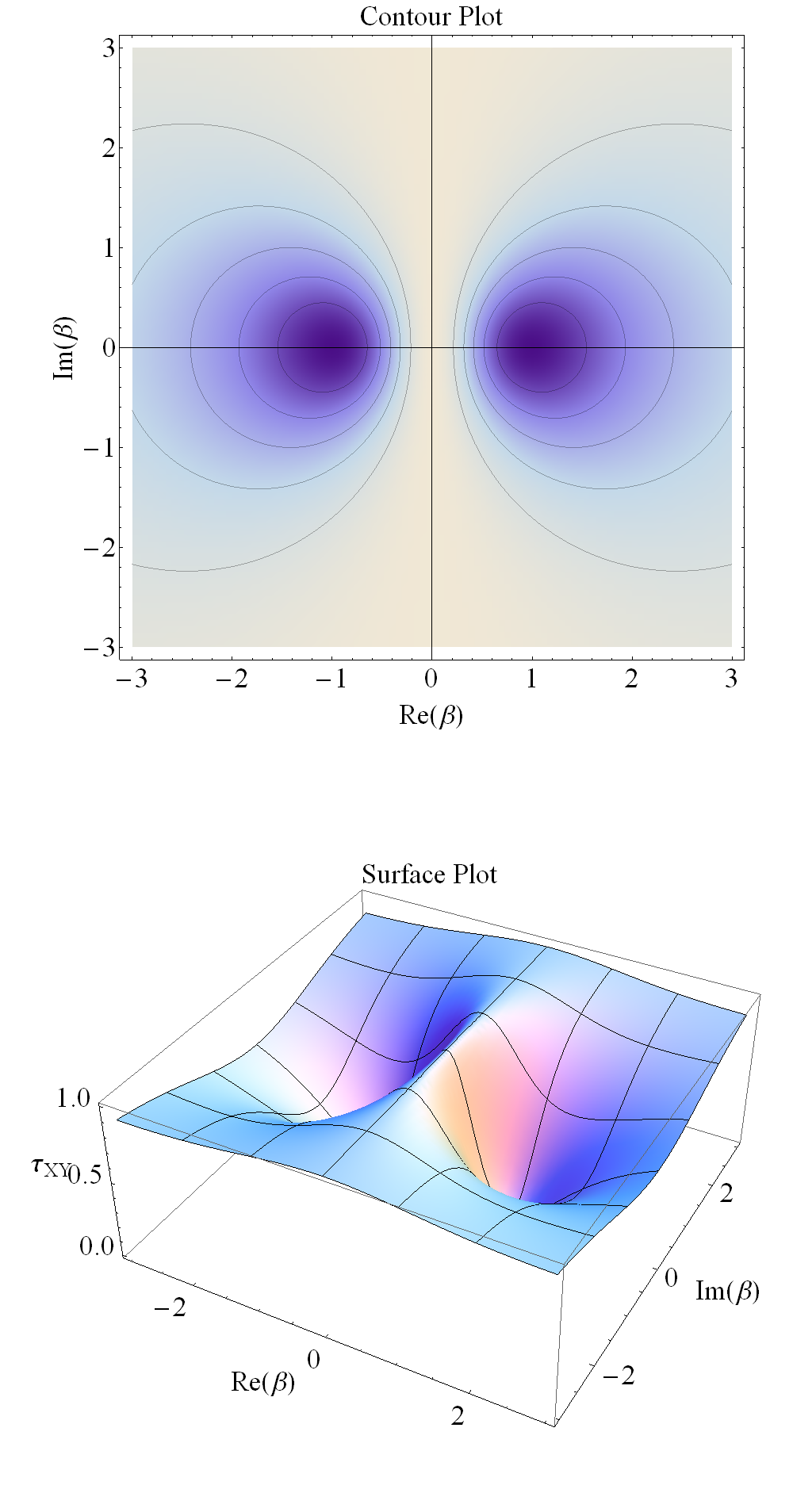
The entanglement for this state is displayed as a function of the complex parameter β\beta in Figure 3 for the case α=1\alpha=1.

Refer to caption
Figure 3: The 2-tangle τX​Y\tau_{XY} for the state (107) for a complex parameter β\beta.

Note, in particular, that while the entanglement is maximized for arbitrary pure imaginary β\beta, it has its minimum value on the real axis at β=±1\beta=\pm 1 as shown in Figure 4.

Figure 4: The 2-tangle τX​Y\tau_{XY} for the state (107) for a real parameter β\beta.

V.2 Three superqubits

In seeking to generalize the 3-tangle (39), invariant under [S​L​(2)]3[SL(2)]^{3}, to a supersymmetric object, invariant under [O​S​p​(1|2)]3[OSp(1|2)]^{3}, we need to find a quartic polynomial that reduces to Cayley’s hyperdeterminant when aAB∙a_{AB\bullet}, aA∙Ca_{A\bullet C}, a∙B​Ca_{\bullet BC}, aA∙∙a_{A\bullet\bullet}, a∙B∙a_{\bullet B\bullet}, a∙∙Ca_{\bullet\bullet C}, and a∙∙∙a_{\bullet\bullet\bullet} are set to zero. We do this by generalizing the γ\gamma matrices:

γA1​A2:=aA1B​CaA2​B​C−aA1B∙aA2B∙−aA1∙CaA2∙C−aA1∙⁣∙aA2∙∙,\displaystyle\begin{split}\gamma_{A_{1}A_{2}}:=&\phantom{-\ }a_{A_{1}}{}^{BC}a_{A_{2}BC}-a_{A_{1}}{}^{B\bullet}a_{A_{2}B\bullet}\\ &-a_{A_{1}}{}^{\bullet C}a_{A_{2}\bullet C}-a_{A_{1}}{}^{\bullet\bullet}a_{A_{2}\bullet\bullet},\end{split} (109a)
γA1∙:=aA1B​Ca∙B​C+aA1B∙a∙B∙+aA1∙Ca∙∙C−aA1∙⁣∙a∙∙∙,\displaystyle\begin{split}\gamma_{A_{1}\bullet}:=&\phantom{-\ }a_{A_{1}}{}^{BC}a_{\bullet BC}+a_{A_{1}}{}^{B\bullet}a_{\bullet B\bullet}\\ &+a_{A_{1}}{}^{\bullet C}a_{\bullet\bullet C}-a_{A_{1}}{}^{\bullet\bullet}a_{\bullet\bullet\bullet},\end{split} (109b)
γ∙A2:=a∙B​CaA2​B​C−a∙B∙aA2B∙−a∙∙CaA2∙C−a∙∙⁣∙aA2∙∙,\displaystyle\begin{split}\gamma_{\bullet A_{2}}:=&\phantom{-\ }a_{\bullet}{}^{BC}a_{A_{2}BC}-a_{\bullet}{}^{B\bullet}a_{A_{2}B\bullet}\\ &-a_{\bullet}{}^{\bullet C}a_{A_{2}\bullet C}-a_{\bullet}{}^{\bullet\bullet}a_{A_{2}\bullet\bullet},\end{split} (109c)

together with their BB and CC counterparts; notice that the building blocks with two indices are bosonic and those with one index are fermionic. The final bosonic possibility, γ(∙∙)\gamma_{(\bullet\bullet)}, vanishes identically. The simple supersymmetry relations are given by

QA1​γA2​A3=εA1​(A2CLOSEγA3)∙QA1γA2∙=12​γA1​A2QB​γA1​A2=0=QC​γA1​A2QBγA∙=0=QCγA∙.\begin{split}Q_{A_{1}}\gamma_{A_{2}A_{3}}&=\varepsilon_{A_{1}(A_{2}}\gamma_{A_{3})\bullet}\\ Q_{A_{1}}\gamma_{A_{2}\bullet}&=\tfrac{1}{2}\gamma_{A_{1}A_{2}}\\ Q_{B}\gamma_{A_{1}A_{2}}&=0=Q_{C}\gamma_{A_{1}A_{2}}\\ Q_{B}\gamma_{A\bullet}&=0=Q_{C}\gamma_{A\bullet}.\end{split} (110)

Using these expressions we define the superhyperdeterminant, denoted sDet⁡a\sDet a:

sDetaX​Y​Z=12(γA1​A2γA1​A2−γA∙γA∙−γ∙Aγ∙A)\sDet a_{XYZ}=\tfrac{1}{2}(\gamma^{A_{1}A_{2}}\gamma_{A_{1}A_{2}}-\gamma^{A\bullet}\gamma_{A\bullet}-\gamma^{\bullet A}\gamma_{\bullet A}) (111)

which is invariant under the action of the superalgebra. The corresponding expressions singling out superqubits BB and CC are also invariant and equal to (111). sDet⁡aX​Y​Z\sDet a_{XYZ} can be seen as the definition of the super-Cayley determinant of the cubic superhypermatrix given in Figure 2.

Writing

ΓA:=(γA1​A2γA1∙γ∙A2γ∙⁣∙)=(γA1​A2γA1∙γA2∙0),\Gamma^{A}:=\begin{pmatrix}\gamma_{A_{1}A_{2}}&\vrule&\gamma_{A_{1}\bullet}\\ \hline\cr\gamma_{\bullet A_{2}}&\vrule&\gamma_{\bullet\bullet}\end{pmatrix}=\begin{pmatrix}\gamma_{A_{1}A_{2}}&\vrule&\gamma_{A_{1}\bullet}\\ \hline\cr\gamma_{A_{2}\bullet}&\vrule&0\end{pmatrix}, (112)

we obtain an invariant analogous to (100)

sDet⁡aX​Y​Z=12​str⁡[(ΓA​E)s​t​E​ΓA]\sDet a_{XYZ}=\tfrac{1}{2}\str[(\Gamma^{A}E)^{st}E\Gamma^{A}] (113)

so that

sDet⁡aX​Y​Z=−sdet⁡ΓA\sDet a_{XYZ}=-\sdet\Gamma^{A} (114)

in analogy to the conventional three-qubit identity (38). This result for sDet agrees with that of [7].

Finally, using ΓA\Gamma^{A} we are able to define the supersymmetric generalization TX​Y​ZT_{XYZ} of the 3-qubit tensor TA​B​CT_{ABC} as defined in (37),

TX​Y​Z=ΓX​X′A​a​Y​ZX′​.T_{XYZ}=\Gamma^{A}_{XX^{\prime}}a^{{{X^{\prime}}\mathchoice{\makebox[12.36185pt][c]{$\displaystyle$}}{\makebox[12.36185pt][c]{$\textstyle$}}{\makebox[7.62901pt][c]{$\scriptstyle$}}{\makebox[5.44928pt][c]{$\scriptscriptstyle$}}}}_{{\mathchoice{\makebox[8.9496pt][c]{$\displaystyle$}}{\makebox[8.9496pt][c]{$\textstyle$}}{\makebox[5.90651pt][c]{$\scriptstyle$}}{\makebox[4.6368pt][c]{$\scriptscriptstyle$}}{YZ}}}. (115)

It is not difficult to verify that TX​Y​ZT_{XYZ} transforms in precisely the same way as aX​Y​Za_{XYZ} (as given in Table 4) under 𝔬​𝔰​𝔭​(1|2)⊕𝔬​𝔰​𝔭​(1|2)⊕𝔬​𝔰​𝔭​(1|2)\mathfrak{osp}(1|2)\oplus\mathfrak{osp}(1|2)\oplus\mathfrak{osp}(1|2). The superhyperdeterminant may then also be written as

sDet⁡aX​Y​Z=TA​B​C​aA​B​C+T∙B​C​a∙B​C−TA∙CaA∙C−TAB∙aAB∙−TA∙∙aA∙∙+T∙B∙a∙B∙+T∙∙Ca∙∙C−T∙∙∙a∙∙∙.\begin{split}\sDet a_{XYZ}&=T_{ABC}a^{ABC}+T_{\bullet BC}a^{\bullet BC}\\ &\phantom{=}-T_{A\bullet C}a^{A\bullet C}-T_{AB\bullet}a^{AB\bullet}\\ &\phantom{=}-T_{A\bullet\bullet}a^{A\bullet\bullet}+T_{\bullet B\bullet}a^{\bullet B\bullet}\\ &\phantom{=}+T_{\bullet\bullet C}a^{\bullet\bullet C}-T_{\bullet\bullet\bullet}a^{\bullet\bullet\bullet}.\end{split} (116)

In this sense sDet⁡aX​Y​Z\sDet a_{XYZ}, (ΓA)X1​X2(\Gamma^{A})_{X_{1}X_{2}}, and TX​Y​ZT_{XYZ} are the natural supersymmetric generalizations of the hyperdeterminant, Det⁡aA​B​C\Det a_{ABC}, and the covariant tensors, (γA)A1​A2(\gamma^{A})_{A_{1}A_{2}} and TA​B​CT_{ABC}, of the conventional 3-qubit treatment summarized in subsection III.2. Finally we are in a position to define the super 3-tangle:

τX​Y​Z=4​sDet⁡aX​Y​Z​(sDet⁡aX​Y​Z)#.\tau_{XYZ}=4\sqrt{\sDet a_{XYZ}(\sDet a_{XYZ})^{\#}.} (117)

In summary 3-superqubit entanglement seems to have the same five entanglement classes as that of 3-qubits shown in Table 1, with the covariants aA​B​C,γA,γB,γC,TA​B​Ca_{ABC},\gamma^{A},\gamma^{B},\gamma^{C},T_{ABC} and Det⁡aA​B​C\Det a_{ABC} replaced by their supersymmetric counterparts aX​Y​Z,ΓA,ΓB,ΓC,TX​Y​Za_{XYZ},\Gamma^{A},\Gamma^{B},\Gamma^{C},T_{XYZ} and sDet⁡aA​B​C\sDet a_{ABC}.

Completely separable nonsuperentangled states are given by product states for which aA​B​C=aAbBcC,aAB∙=aAbBc∙,aA∙C=aAb∙cC,a∙B​C=a∙bBcC,aA∙∙=aAb∙c∙,a∙B∙=a∙bBc∙,a∙∙C=a∙b∙cC,a∙∙∙=a∙b∙c∙a_{ABC}=a_{A}b_{B}c_{C},a_{AB\bullet}=a_{A}b_{B}c_{\bullet},a_{A\bullet C}=a_{A}b_{\bullet}c_{C},a_{\bullet BC}=a_{\bullet}b_{B}c_{C},a_{A\bullet\bullet}=a_{A}b_{\bullet}c_{\bullet},a_{\bullet B\bullet}=a_{\bullet}b_{B}c_{\bullet},a_{\bullet\bullet C}=a_{\bullet}b_{\bullet}c_{C},a_{\bullet\bullet\bullet}=a_{\bullet}b_{\bullet}c_{\bullet}, and sDet⁡aX​Y​Z\sDet a_{XYZ} vanishes. This provides a nontrivial consistency check.

An example of a normalized physical biseparable state is provided by

|Ψ⟩=13(|000⟩+|011⟩+|0∙∙⟩)\lvert\Psi\rangle=\tfrac{1}{\sqrt{3}}(\lvert 000\rangle+\lvert 011\rangle+\lvert 0\bullet\bullet\rangle) (118)

for which

(ΓA)00=13(\Gamma^{A})_{00}=\tfrac{1}{3} (119)

and ΓB\Gamma^{B}, ΓC\Gamma^{C}, TX​Y​ZT_{XYZ} and sDet⁡aX​Y​Z\sDet a_{XYZ} vanish. More generally, one can consider the combination

|Ψ⟩=(|α|2+|β|2)−1/2[12α(|000⟩+|011⟩)+β|0∙∙⟩]\lvert\Psi\rangle=(|\alpha|^{2}+|\beta|^{2})^{-1/2}[\tfrac{1}{\sqrt{2}}\alpha(\lvert 000\rangle+\lvert 011\rangle)+\beta\lvert 0\bullet\bullet\rangle] (120)

for which

(ΓA)00=α2−β2|α|2+|β|2(\Gamma^{A})_{00}=\frac{\alpha^{2}-\beta^{2}}{|\alpha|^{2}+|\beta|^{2}} (121)

and the other covariants vanish.

An example of a normalized physical W state is provided by

|Ψ⟩=16(|110⟩+|101⟩+|011⟩+|∙∙1⟩+|∙1∙⟩+|1∙∙⟩)\begin{split}\lvert\Psi\rangle=\tfrac{1}{\sqrt{6}}(&\lvert 110\rangle+\lvert 101\rangle+\lvert 011\rangle\\ +&\lvert\bullet\bullet 1\rangle+\lvert\bullet 1\bullet\rangle+\lvert 1\bullet\bullet\rangle)\end{split} (122)

for which

(ΓA)11=(ΓB)11=(ΓC)11=−12(\Gamma^{A})_{11}=(\Gamma^{B})_{11}=(\Gamma^{C})_{11}=-\tfrac{1}{2} (123)

and

T111=12​6T_{111}=\tfrac{1}{2\sqrt{6}} (124)

while sDet⁡aX​Y​Z\sDet a_{XYZ} vanishes. One could also consider

|Ψ⟩=13(|α|2+|β|2)−1/2[α(|110⟩+|101⟩+|011⟩)+β(|∙∙1⟩+|∙1∙⟩+|1∙∙⟩)]\begin{split}\lvert\Psi\rangle=\tfrac{1}{\sqrt{3}}(|\alpha|^{2}+|\beta|^{2})^{-1/2}[&\alpha(\lvert 110\rangle+\lvert 101\rangle+\lvert 011\rangle)\\ +&\beta(\lvert\bullet\bullet 1\rangle+\lvert\bullet 1\bullet\rangle+\lvert 1\bullet\bullet\rangle)]\end{split} (125)

for which

(ΓA)11=(ΓB)11=(ΓC)11=−2​α2+β23​(|α|2+|β|2)(\Gamma^{A})_{11}=(\Gamma^{B})_{11}=(\Gamma^{C})_{11}=-\frac{2\alpha^{2}+\beta^{2}}{3(|\alpha|^{2}+|\beta|^{2})} (126)

and

T111=α⁡(2​α2+β2)3​3​(|α|2+|β|2)3/2T_{111}=\frac{\alpha(2\alpha^{2}+\beta^{2})}{3\sqrt{3}(|\alpha|^{2}+|\beta|^{2})^{3/2}} (127)

while the other TT components and sDet⁡aX​Y​Z\sDet a_{XYZ} vanish.

An example of a normalized physical superentangled state is provided by

|Ψ⟩=18(|000⟩+|∙∙0⟩+|∙0∙⟩+|0∙∙⟩+|111⟩+|∙∙1⟩+|∙1∙⟩+|1∙∙⟩)\begin{split}\lvert\Psi\rangle=\tfrac{1}{\sqrt{8}}(&\lvert 000\rangle+\lvert\bullet\bullet 0\rangle+\lvert\bullet 0\bullet\rangle+\lvert 0\bullet\bullet\rangle\\ +&\lvert 111\rangle+\lvert\bullet\bullet 1\rangle+\lvert\bullet 1\bullet\rangle+\lvert 1\bullet\bullet\rangle)\end{split} (128)

for which

sDet⁡aX​Y​Z=164\sDet a_{XYZ}=\tfrac{1}{64} (129)

and

τX​Y​Z=4​sDet⁡aX​Y​Z​(sDet⁡aX​Y​Z)#=116.\tau_{XYZ}=4\sqrt{\sDet a_{XYZ}(\sDet a_{XYZ})^{\#}}=\tfrac{1}{16}. (130)

VI Conclusion

In this paper we have taken the first steps toward generalizing quantum information theory to super quantum information theory. We introduced the superqubit defined over an appropriate super Hilbert space. We acknowledge that there are still important issues to address, notably how to interpret “physical” states with nonvanishing soul for which probabilities are no longer real numbers but elements of a Grassmann algebra. (The sum of the probabilities still add up to one, however.) The examples of section V avoided this problem, being pure body. DeWitt advocates retaining only such pure body states in the Hilbert space [23], but this may be too draconian. See [27] for an alternative approach.

Nevertheless, for the SLOCC equivalence group [S​L​(2,ℂ)]n[SL(2,\mathds{C})]^{n} and the LOCC equivalence group [S​U​(2)]n[SU(2)]^{n}, we presented their minimal supersymmetric extensions, [O​S​p​(1|2)]n[OSp(1|2)]^{n} and [u​O​S​p​(1|2)]n[uOSp(1|2)]^{n} respectively, and showed explicitly how superqubits would transform under these groups for n=1,2,3n=1,2,3. Furthermore, we found supersymmetric invariants that are the obvious candidates for supersymmetric entanglement measures for n=2,3n=2,3. We hope in future work to classify fully the 2 and 3 superqubit entanglement classes and their corresponding orbits as was done for the 2 and 3 qubit entanglement classes in [2, 4, 6].

As noted in the Introduction, a physical realization of our superqubit is more likely to be found in condensed-matter physics than high-energy physics. While the polarizations of a photon or the spins of an electron provide examples of a qubit, the inclusions of photinos or selectrons do not obviously provide examples of a superqubit, since the supersymmetrization of the (S)LOCC equivalence groups is distinct from the supersymmetrization of the spacetime Poincaré group.

We would also like to point out that this work is part of the ongoing correspondence between ideas in string and M-theory and ideas in quantum information theory. See [28] for a review. This paper continues the trend of using mathematical tools from one side to describe phenomena on the other.

Acknowledgements.
We are grateful to L. Castellani, P. A. Grassi, and L. Sommovigo for useful correspondence, to S. Bellucci for helpful discussions, and to Kazuki Hasebe for alerting us to the supersymmetric tt-JJ model. This work was supported in part by the STFC under rolling Grant No. ST/G000743/1.

Note added

A very interesting paper has recently appeared [29], which analyzes quantum computing with superqubits.

Appendix A Superlinear algebra

Grassmann numbers are the 2n2^{n}-dimensional vectors populating the Grassmann algebra Λn\Lambda_{n}, which is generated by nn mutually anticommuting elements {θi}i=1n\{\theta^{i}\}_{i=1}^{n}.

Any Grassmann number zz may be decomposed into “body” zℬ∈ℂz_{\mathcal{B}}\in\mathds{C} and “soul” z𝒮z_{\mathcal{S}} viz.

z=zℬ+z𝒮z𝒮=∑k=1∞1k!ca1⋯akθa1⋯θak,\begin{split}z&=z_{\mathcal{B}}+z_{\mathcal{S}}\\ z_{\mathcal{S}}&=\textstyle\sum_{k=1}^{\infty}\tfrac{1}{k!}c_{a_{1}\cdots a_{k}}\theta^{a_{1}}\cdots\theta^{a_{k}},\end{split} (131)

where ca1⋯ak∈ℂc_{a_{1}\cdots a_{k}}\in\mathds{C} are totally antisymmetric. For finite dimension nn the sum terminates at k=2nk=2^{n} and the soul is nilpotent z𝒮n+1=0z_{\mathcal{S}}^{n+1}=0.

One may also decompose zz into even and odd parts uu and vv

u=zℬ+∑k=1∞1(2​k)!ca1⋯a2​kθa1⋯θa2​kv=∑k=0∞1(2​k+1)!ca1⋯a2​k+1θa1⋯θa2​k+1,\begin{split}u&=z_{\mathcal{B}}+\textstyle\sum_{k=1}^{\infty}\tfrac{1}{(2k)!}c_{a_{1}\cdots a_{2k}}\theta^{a_{1}}\cdots\theta^{a_{2k}}\\ v&=\textstyle\sum_{k=0}^{\infty}\tfrac{1}{(2k+1)!}c_{a_{1}\cdots a_{2k+1}}\theta^{a_{1}}\cdots\theta^{a_{2k+1}},\end{split} (132)

which may also be expressed as the direct sum decomposition Λn=Λn0⊕Λn1\Lambda_{n}=\Lambda_{n}^{0}\oplus\Lambda_{n}^{1}. Furthermore, analytic functions ff of Grassmann numbers are defined via

f⁡(z):=∑k=0∞1k!​f(k)​(zℬ)​z𝒮k,f(z):=\sum_{k=0}^{\infty}\tfrac{1}{k!}f^{(k)}(z_{\mathcal{B}})z_{\mathcal{S}}^{k}, (133)

where f(k)​(zℬ)f^{(k)}(z_{\mathcal{B}}) is the kthk^{\textrm{th}} derivative of ff evaluated at zℬz_{\mathcal{B}} and is well defined if ff is nonsingular at zℬz_{\mathcal{B}} [23].

One defines the grade of a Grassmann number as

deg⁡x:={0x∈Λn01x∈Λn1,\deg x:=\begin{cases}0&x\in\Lambda_{n}^{0}\\ 1&x\in\Lambda_{n}^{1},\end{cases} (134)

where the grades 0 and 1 are referred to as even and odd, respectively.

Define the star ⋆ and superstar # operators [30, 26, 25] satisfying the following properties:

(Λn0)⋆=Λn0,(Λn1)⋆=Λn1,(Λn0)#=Λn0,(Λn1)#=Λn1,(x​θi)⋆=x∗​θi⋆,θi⋆⁣⋆=θi,(θi​θj)⋆=θj⋆​θi⋆,(x​θi)#=x∗​θi#,θi#​#=−θi,(θi​θj)#=θi#​θj#,\begin{gathered}\begin{aligned} (\Lambda_{n}^{0})^{\star}&=\Lambda_{n}^{0},&(\Lambda_{n}^{1})^{\star}&=\Lambda_{n}^{1},\\ (\Lambda_{n}^{0})^{\#}&=\Lambda_{n}^{0},&(\Lambda_{n}^{1})^{\#}&=\Lambda_{n}^{1},\end{aligned}\\ \begin{aligned} (x\theta_{i})^{\star}&=x^{*}\theta_{i}^{\star},&\theta_{i}^{\star\star}&=\theta_{i},&(\theta_{i}\theta_{j})^{\star}&=\theta_{j}^{\star}\theta_{i}^{\star},\\ (x\theta_{i})^{\#}&=x^{*}\theta_{i}^{\#},&\theta_{i}^{\#\#}&=-\theta_{i},&(\theta_{i}\theta_{j})^{\#}&=\theta_{i}^{\#}\theta_{j}^{\#},\end{aligned}\end{gathered} (135)

where x∈ℂx\in\mathds{C} and ∗ is ordinary complex conjugation, which means

α⋆⁣⋆\displaystyle\alpha^{\star\star} =α,\displaystyle=\alpha, α#​#\displaystyle\alpha^{\#\#} =(−)deg⁡α​α\displaystyle=(-)^{\deg\alpha}\alpha (136)

for pure even/odd Grassmann α\alpha. The impure case follows by linearity.

Following [23] one may, if so desired, take the formal limit n→∞n\to\infty defining the infinite dimensional vector space Λ∞\Lambda_{\infty}. Elements of Λ∞\Lambda_{\infty} are called supernumbers. Our results are independent of the dimension of the underlying Grassmann algebra and one can use supernumbers throughout, but for the sake of simplicity we restrict to finite dimensional algebra by assigning just one Grassmann generator θ\theta and its superconjugate θ#\theta^{\#} to every superqubit.

The grade definition applies to the components TX1⋯XkT_{X_{1}\cdots X_{k}} of any kk-index array of Grassmann numbers TT, but one may also define deg⁡Xi\deg X_{i}, the grade of an index, for such an array by specifying a characteristic function from the range of the index XiX_{i} to the set {0,1}\{0,1\}. In general the indices can have different ranges and the characteristic functions can be arbitrary for each index. It is then possible to define deg⁡T\deg T, the grade of an array, as long as the compatibility condition

degT≡deg(TX1⋯Xk)+∑i=1kdegXimod2∀Xi\deg T\equiv\deg(T_{X_{1}\cdots X_{k}})+\sum_{i=1}^{k}\deg X_{i}\mod 2\quad\forall\ X_{i} (137)

is satisfied. In precisely such cases the entries of TT satisfy

deg(TX1⋯Xk)=degT+∑i=1kdegXimod2,⟹deg⁡T=deg⁡(T1⋯1⏟k),deg⁡(T1​T2)=deg⁡T1+deg⁡T2mod2,\begin{gathered}\deg(T_{X_{1}\cdots X_{k}})=\deg T+\sum_{i=1}^{k}\deg X_{i}\mod 2,\\ \implies\deg T=\deg(T_{\underbrace{1\cdots 1}_{k}}),\\ \deg(T_{1}T_{2})=\deg T_{1}+\deg T_{2}\mod 2,\end{gathered} (138)

so that in other words TT is partitioned into blocks with definite grade such that the nearest neighbors of any block are of the opposite grade to that block. The array grade simply distinguishes the two distinct ways of accomplishing such a partition (i.e. the two possible grades of the first element T1⋯1T_{1\cdots 1}). Grassmann numbers and the Grassmann number grade may be viewed as special cases of arrays and the array grade.

Special care must be taken not to confuse this notion of array grade with whether the array entries at even/odd index positions vanish. An array TT may be decomposed as

T=TE+TO,T=T_{E}+T_{O}, (139)

where the pure even part TET_{E} is obtained from TT by setting to zero all entries satisfying deg(TX1⋯Xk)=1\deg(T_{X_{1}\cdots X_{k}})=1, and similarly mutatis mutandis for TOT_{O}. The property of being pure even or pure odd is therefore independent of the array grade as defined above.

The various grades commonly appear in formulae as powers of -1 and the shorthand

(−)X:=(−1)deg⁡X(-)^{X}:=(-1)^{\deg X} (140)

is often used. The indices of superarrays may be supersymmetrized as follows:

TX1⋯[[Xi|⋯|Xj]]⋯Xk:=12[TX1⋯Xi⋯Xj⋯Xk+(−)Xi​XjTX1⋯Xj⋯Xi⋯Xk].\begin{gathered}T_{X_{1}\cdots[\![X_{i}|\cdots|X_{j}]\!]\cdots X_{k}}:=\\ \tfrac{1}{2}[T_{X_{1}\cdots X_{i}\cdots X_{j}\cdots X_{k}}+(-)^{X_{i}X_{j}}T_{X_{1}\cdots X_{j}\cdots X_{i}\cdots X_{k}}].\end{gathered} (141)

While we require these definitions for some of our considerations, one typically only uses arrays with 0, 1, or 2 indices where the characteristic functions are monotonic: supernumbers, supervectors, and supermatrices, respectively. Functions of grades extend to mixed superarrays (with nonzero even and odd parts) by linearity.

A (p|q)×(r|s)(p|q)\times(r|s) supermatrix is just an (p+q)×(r+s)(p+q)\times(r+s)-dimensional block partitioned matrix

M=   (rspABqCD)  M=\hbox{}\vbox{\kern 0.86108pt\hbox{$\kern 0.0pt\kern 2.5pt\kern-5.0pt\left(\kern 0.0pt\kern-2.5pt\kern-6.66669pt\vbox{\kern-0.86108pt\vbox{\vbox{\halign{\kern\arraycolsep\hfil\@arstrut$\kbcolstyle#$\hfil\kern\arraycolsep& \kern\arraycolsep\hfil$\@kbrowstyle#$\ifkbalignright\relax\else\hfil\fi\kern\arraycolsep&& \kern\arraycolsep\hfil$\@kbrowstyle#$\ifkbalignright\relax\else\hfil\fi\kern\arraycolsep\cr 5.0pt\hfil\hbox{\vrule height=0.0pt,depth=0.0pt,width=0.0pt}$\scriptstyle$\hfil\kern 5.0pt&5.0pt\hfil$\scriptstyle r$\hfil\kern 5.0pt&5.0pt\hfil$\scriptstyle\vrule$\hfil\kern 5.0pt&5.0pt\hfil$\scriptstyle s$\hfil\kern 5.0pt\\ 5.0pt\hfil\hbox{\vrule height=0.0pt,depth=0.0pt,width=0.0pt}$\scriptstyle p$\hfil\kern 5.0pt&5.0pt\hfil$\scriptstyle A$\hfil\kern 5.0pt&5.0pt\hfil$\scriptstyle\vrule$\hfil\kern 5.0pt&5.0pt\hfil$\scriptstyle B$\hfil\kern 5.0pt\\ \hline\cr 5.0pt\hfil\hbox{\vrule height=0.0pt,depth=0.0pt,width=0.0pt}$\scriptstyle q$\hfil\kern 5.0pt&5.0pt\hfil$\scriptstyle C$\hfil\kern 5.0pt&5.0pt\hfil$\scriptstyle\vrule$\hfil\kern 5.0pt&5.0pt\hfil$\scriptstyle D$\hfil\kern 5.0pt\crcr}}}}\right)$}} (142)

where entries in the AA and DD blocks are grade deg⁡M\deg M, and those in the BB and CC blocks are grade deg⁡M+1mod2\deg M+1\mod 2. The special cases s=0s=0 or q=0q=0 can be permitted to make the definition encapsulate row and column supervectors. Supermatrix multiplication is defined as for ordinary matrices; however, the trace, transpose, adjoint, and determinant have distinct super versions [25, 31].

The supertrace str⁡M\str M of a supermatrix is MM defined as

str⁡M:=∑X(−)(X+M)​X​MX​X\str M:=\sum_{X}(-)^{(X+M)X}M_{XX} (143)

and is linear, cyclic modulo sign, and insensitive to the supertranspose

str⁡(M+N)=str⁡(M)+str⁡(N)str⁡(M​N)=(−)M​N​str⁡(N​M)str⁡Ms​t=str⁡M.\begin{split}\str(M+N)&=\str(M)+\str(N)\\ \str(MN)&=(-)^{MN}\str(NM)\\ \str M^{st}&=\str M.\end{split} (144)

The supertranspose Ms​tM^{st} of a supermatrix MM is defined componentwise as

Ms​t:=X1​X2(−)(X2+M)​(X1+X2)MX2​X1.M^{st}{}_{X_{1}X_{2}}:=(-)^{(X_{2}+M)(X_{1}+X_{2})}M_{X_{2}X_{1}}. (145)

Unlike the transpose the supertranspose is not idempotent; instead,

Ms​t​s​tX1​X2=(−)(X1+X2)​MX1​X2,Ms​t​s​t​s​tX1​X2=(−)(X1+M)​(X1+X2)​MX2​X1,Ms​t​s​t​s​t​s​tX1​X2=MX1​X2,\begin{split}M^{st\,st}{}_{X_{1}X_{2}}&=(-)^{(X_{1}+X_{2})}M_{X_{1}X_{2}},\\ M^{st\,st\,st}{}_{X_{1}X_{2}}&=(-)^{(X_{1}+M)(X_{1}+X_{2})}M_{X_{2}X_{1}},\\ M^{st\,st\,st\,st}{}_{X_{1}X_{2}}&=M_{X_{1}X_{2}},\end{split} (146)

so that it is of order 4. The supertranspose also satisfies

(M​N)s​t=(−)M​N​Ns​t​Ms​t.(MN)^{st}=(-)^{MN}N^{st}M^{st}. (147)

The adjoint † and superadjoint ‡ of a supermatrix are defined as

M†:=M⋆tM‡:=M#​s​t,\begin{split}M^{\dagger}&:=M^{\star t}\\ M^{\ddagger}&:=M^{\#st},\end{split} (148)

and satisfy

M†⁣†\displaystyle M^{{\dagger}{\dagger}} =M,\displaystyle=M, M‡⁣‡\displaystyle M^{{\ddagger}{\ddagger}} =(−)M​M,\displaystyle=(-)^{M}M, (149)
(M​N)†\displaystyle(MN)^{\dagger} =N†​M†,\displaystyle=N^{\dagger}M^{\dagger}, (M​N)‡\displaystyle(MN)^{\ddagger} =(−)M​N​N‡​M‡.\displaystyle=(-)^{MN}N^{\ddagger}M^{\ddagger}.

The preservation of anti-super-Hermiticity, M‡=−MM^{\ddagger}=-M, under scalar multiplication by Grassmann numbers, as required for the proper definition of 𝔲​𝔬​𝔰​𝔭​(1|2)\mathfrak{uosp}(1|2) [32], necessitates the left/right multiplication rules:

(α​M)X1​X2=(−)X1​α​α​MX1​X2,(M​α)X1​X2=(−)X2​α​MX1​X2​α.\begin{split}(\alpha M)_{X_{1}X_{2}}&=(-)^{X_{1}\alpha}\alpha M_{X_{1}X_{2}},\\ (M\alpha)_{X_{1}X_{2}}&=(-)^{X_{2}\alpha}M_{X_{1}X_{2}}\alpha.\end{split} (150)

The Berezinian is defined as

Ber⁡M:=det(A−B​D−1​C)/det(D)=det(A)/det(D−C​A−1​B)\begin{split}\Ber M&:=\det(A-BD^{-1}C)/\det(D)\\ &=\det(A)/\det(D-CA^{-1}B)\end{split} (151)

and is multiplicative, insensitive to the supertranspose, and generalizes the relationship between trace and determinant

Ber⁡(M​N)=Ber⁡(M)​Ber⁡(N)Ber⁡Ms​t=Ber⁡MBer⁡eM=estr⁡M.\begin{split}\Ber(MN)&=\Ber(M)\Ber(N)\\ \Ber M^{st}&=\Ber M\\ \Ber e^{M}&=e^{\str M}.\end{split} (152)

The direct sum and super tensor product are unchanged from their ordinary versions. As such, the dimension of the tensor product of two superqubits is given by

(2|1)⊗(2|1)=(2​|1|​2​|3|​1),(2|1)\otimes(2|1)=(2|1|2|3|1), (153)

while the threefold product is

(2|1)⊗3=(2|1​|2​|3​|3​|1​|2​|3|​1|​2|​1|​2|​3|​1),(2|1)^{\otimes 3}=(2|1|2|3|3|1|2|3|1|2|1|2|3|1), (154)

with similar results holding for the associated density matrices. In analogy with the ordinary case we have

(M⊗N)t=Mt⊗Nt(M⊗N)s​t=Ms​t⊗Ns​tstr⁡(M⊗N)=str⁡M​str⁡N.\begin{split}(M\otimes N)^{t}&=M^{t}\otimes N^{t}\\ (M\otimes N)^{st}&=M^{st}\otimes N^{st}\\ \str(M\otimes N)&=\str M\str N.\end{split} (155)

These definitions are manifestly compatible with Hermiticity and super-Hermiticity.

Denoting the total number of bosonic elements in the product of nn superqubits by BnB_{n}, and similarly the total number of fermionic elements by FnF_{n}, we know that BnB_{n} (FnF_{n}) is given by the total number of basis kets with an even (odd) number of ∙\bullet’s:

Bn=(n0)​2n+(n2)​2n−2+⋯=3n+12Fn=(n1)​2n−1+(n3)​2n−3+⋯=3n−12\begin{split}B_{n}&={n\choose 0}2^{n}+{n\choose 2}2^{n-2}+\cdots=\frac{3^{n}+1}{2}\\ F_{n}&={n\choose 1}2^{n-1}+{n\choose 3}2^{n-3}+\cdots=\frac{3^{n}-1}{2}\end{split} (156)

so that, in particular, Bn−Fn=1B_{n}-F_{n}=1: the number of bosonic elements is always one more than the number of fermionic ones.

In supermatrix representations of superalgebras, one may represent the superbracket of generators MM and NN as

[[M,N]]:=M​N−NE​M−NO​(ME−MO).[\![M,N]\!]:=MN-N_{E}M-N_{O}(M_{E}-M_{O}). (157)

One may also consider supermatrices MM and NN whose components are themselves supermatrices. Provided the component supermatrices are pure even (odd) at even (odd) index positions (e.g. M11M_{11} is a pure even supermatrix for even MM), one may write the superbracket of such supermatrices as

[[MX1​X2,NX3​X4]]=MX1​X2​NX3​X4−(−)(X1+X2)​(X3+X4)​NX3​X4​MX1​X2,\begin{gathered}[\![M_{X_{1}X_{2}},N_{X_{3}X_{4}}]\!]=\\ M_{X_{1}X_{2}}N_{X_{3}X_{4}}-(-)^{(X_{1}+X_{2})(X_{3}+X_{4})}N_{X_{3}X_{4}}M_{X_{1}X_{2}},\end{gathered} (158)

where the final two indices are suppressed. This grouping of supermatrices into supermatrices is useful for summarizing the superbrackets of superalgebras.

Appendix B Orthosymplectic superalgebras

Supermatrix representations of the orthosymplectic supergroup O​S​p​(p|2​q)OSp(p|2q) consist of supermatrices M∈G​L​(p|2​q)M\in GL(p|2q) satisfying

Ms​t​E​M=E,M^{st}EM=E, (159)

but for convenience we choose instead to use supermatrices M∈G​L​(2​q|p)M\in GL(2q|p) satisfying (159). In this convention, the invariant supermatrix EE is defined by

E\displaystyle E :=(𝕁2​q00𝟙p),\displaystyle:=\begin{pmatrix}\mathds{J}_{2q}&\vrule&0\\ \hline\cr 0&\vrule&\mathds{1}_{p}\end{pmatrix}, 𝕁2​q\displaystyle\mathds{J}_{2q} :=(0𝟙q−𝟙q0).\displaystyle:=\begin{pmatrix}0&\mathds{1}_{q}\\ -\mathds{1}_{q}&0\end{pmatrix}. (160)

Definitions of supermatrices, the supertranspose, and further details of superlinear algebra may be found in Appendix A.

Writing a generic supermatrix 𝔐\mathfrak{M} of the super Lie algebra 𝔬​𝔰​𝔭​(p|2​q)\mathfrak{osp}(p|2q) as

𝔐=(ABCD)\mathfrak{M}=\begin{pmatrix}A&\vrule&B\\ \hline\cr C&\vrule&D\end{pmatrix} (161)

permits (159) to be rewritten as the following conditions on the blocks of the algebra supermatrices:

At​𝕁\displaystyle A^{t}\mathds{J} =−𝕁​A,\displaystyle=-\mathds{J}A, C\displaystyle C =Bt​𝕁,\displaystyle=B^{t}\mathds{J}, Dt\displaystyle D^{t} =−D.\displaystyle=-D. (162)

Depending on the value of pp, the superalgebra falls into one of three basic, “classical” families

𝔬​𝔰​𝔭​(p|2​q)={B⁡(r,q)p=2​r+1,r≥0C⁡(q+1)p=2D⁡(r,q)p=2r,r≥2.\mathfrak{osp}(p|2q)=\begin{cases}B(r,q)&p=2r+1,\ r\geq 0\\ C(q+1)&p=2\\ D(r,q)&p=2r,\ r\geq 2.\end{cases} (163)

Clearly it is the first case that will concern us, in particular, with r=0,q=1r=0,q=1. B⁡(r,q)B(r,q) has rank q+rq+r, dimension 2​(q+r)2+3​q+r2(q+r)^{2}+3q+r, and even part 𝔰​𝔬​(p)⊕𝔰​𝔭​(2​q)\mathfrak{so}(p)\oplus\mathfrak{sp}(2q), which for 𝔬​𝔰​𝔭​(1|2)\mathfrak{osp}(1|2) are 1, 5, and 𝔰​𝔩​(2)\mathfrak{sl}(2), respectively.

One generates 𝔬​𝔰​𝔭​(p|2​q)\mathfrak{osp}(p|2q) as a matrix superalgebra by defining the supermatrices UU and GG

(UX1​X2)X3​X4:=δX1​X4​δX2​X3,G:=(𝕁2​q00Hp),\displaystyle\begin{gathered}(U_{X_{1}X_{2}})_{X_{3}X_{4}}:=\delta_{X_{1}X_{4}}\delta_{X_{2}X_{3}},\\ G:=\begin{pmatrix}\mathds{J}_{2q}&\vrule&0\\ \hline\cr 0&\vrule&H_{p}\end{pmatrix},\end{gathered}
where
Hp:={σ1⊗𝟙rp=2​r[σ1⊗𝟙r]⊕(1)p=2​r+1\displaystyle H_{p}:=\begin{cases}\phantom{[}\sigma_{1}\otimes\mathds{1}_{r}&p=2r\\ [\sigma_{1}\otimes\mathds{1}_{r}]\oplus(1)&p=2r+1\end{cases} (166)

with σ1\sigma_{1} being the first Pauli matrix. Here the indices XiX_{i} range from 1 to 2​q+p2q+p and are partitioned as Xi=(X¯i,X˙i)X_{i}=(\bar{X}_{i},\dot{X}_{i}) with X¯i\bar{X}_{i} ranging from 1 to 2​q2q, and X˙i\dot{X}_{i} taking on the remaining pp values. Note that under (B), GG has the following symmetry properties

GX¯1​X¯2=−GX¯2​X¯1,GX˙1​X˙2=+GX˙2​X˙1,GX¯1​X˙2=0=GX˙2​X¯1,\begin{gathered}\begin{aligned} G_{\bar{X}_{1}\bar{X}_{2}}&=-G_{\bar{X}_{2}\bar{X}_{1}},&G_{\dot{X}_{1}\dot{X}_{2}}&=+G_{\dot{X}_{2}\dot{X}_{1}},\end{aligned}\\ G_{\bar{X}_{1}\dot{X}_{2}}=0=G_{\dot{X}_{2}\bar{X}_{1}},\end{gathered} (167)

which are shared with the invariant supermatrix EE. In the special case p=1p=1, GG reduces to EE.

The generators TT are obtained as

TX1​X2=2G[[X1|X3UX3|X2]],T_{X_{1}X_{2}}=2G_{[\![X_{1}|X_{3}}U_{X_{3}|X_{2}]\!]}, (168)

where TT has array grade zero and the index grades are monotonically increasing:

deg⁡X:={0X∈{1,…,2​q}1X∈{2​q+1,…,2​q+p}.\deg X:=\begin{cases}0&X\in\{1,\dotsc,2q\}\\ 1&X\in\{2q+1,\dotsc,2q+p\}.\end{cases} (169)

Clearly TT has symmetry properties TX1​X2=T[[X1​X2]]T_{X_{1}X_{2}}=T_{[\![X_{1}X_{2}]\!]}. The 2​q​(2​q+1)/22q(2q+1)/2 generators TX¯1​X¯2T_{\bar{X}_{1}\bar{X}_{2}} generate 𝔰​𝔭​(2​q)\mathfrak{sp}(2q), the p⁡(p−1)/2p(p-1)/2 generators TX˙1​X˙2T_{\dot{X}_{1}\dot{X}_{2}} generate 𝔰​𝔬​(p)\mathfrak{so}(p), and both are even (bosonic), while the 2​p​q2pq generators TX¯1​X˙2T_{\bar{X}_{1}\dot{X}_{2}} are odd (fermionic). These supermatrices yield the 𝔬​𝔰​𝔭​(p|2​q)\mathfrak{osp}(p|2q) superbrackets

[[TX1​X2,TX3​X4]]:=4G[[X1[[X3TX2]]X4]],[\![T_{X_{1}X_{2}},T_{X_{3}X_{4}}]\!]:=4G_{[\![X_{1}[\![X_{3}}T_{X_{2}]\!]X_{4}]\!]}, (170)

where the supersymmetrization on the right-hand side is over pairs X1​X2X_{1}X_{2} and X3​X4X_{3}X_{4} as on the left-hand side. The action of the generators on (2​q|p)(2q|p)-dimensional supervectors aXa_{X} is given by

(TX1​X2)X3​X4aX4≡(TX1​X2a)X3=2G[[X1|X3aX2]](T_{X_{1}X_{2}})_{X_{3}X_{4}}a_{X_{4}}\equiv(T_{X_{1}X_{2}}a)_{X_{3}}=2G_{[\![X_{1}|X_{3}}a_{X_{2}]\!]} (171)

This action may be generalized to an NN-fold super tensor product of (2​q|p)(2q|p) supervectors by labeling the indices with integers k=1,2,…,Nk=1,2,\dotsc,N

(TXk​Yka)Z1⋯Zk⋯ZN=(−)(Xk+Yk)​∑i=1k−1|Zi|2G[[Xk|ZkaZ1⋯|Yk]]⋯ZN.\begin{gathered}(T_{X_{k}Y_{k}}a)_{Z_{1}\cdots Z_{k}\cdots Z_{N}}=\\ (-)^{(X_{k}+Y_{k})\sum_{i=1}^{k-1}|Z_{i}|}2G_{[\![X_{k}|Z_{k}}a_{Z_{1}\cdots|Y_{k}]\!]\cdots Z_{N}}.\end{gathered} (172)

In our special case p=1p=1 we denote the lone dotted index X˙i\dot{X}_{i} by a bullet ∙\bullet and start counting the barred indices at zero so that Xi=(0,1,∙)X_{i}=(0,1,\bullet). Obviously the T∙⁣∙T_{\bullet\bullet} generator vanishes identically, leaving only the following superbrackets:

[TA1​A2,TA3​A4]=4​E(A1​(A3CLOSECLOSE​TOPENOPENA2)​A4)[TA1​A2,TA3∙]=2E(A1|A3CLOSETA2)∙{TA1∙,TA2∙}=TA1​A2,\begin{split}\left[T_{A_{1}A_{2}},T_{A_{3}A_{4}}\right]&=4E_{(A_{1}(A_{3}}T_{A_{2})A_{4})}\\ \left[T_{A_{1}A_{2}},T_{A_{3}\bullet}\right]&=2E_{(A_{1}|A_{3}}T_{A_{2})\bullet}\\ \left\{T_{A_{1}\bullet},T_{A_{2}\bullet}\right\}&=T_{A_{1}A_{2}},\end{split} (173)

which are written out in Table 5 with TA≡TA∙≡T∙AT_{A}\equiv T_{A\bullet}\equiv T_{\bullet A}.

Table 5: 𝔬​𝔰​𝔭​(1|2)\mathfrak{osp}(1|2) superbrackets.
T01T_{01} T00T_{00} T11T_{11} T0T_{0} T1T_{1}
T01T_{01} 00 −2​T00-2T_{00} 2​T112T_{11} −T0-T_{0} T1T_{1}
T00T_{00} 2​T002T_{00} 00 4​T014T_{01} 00 2​T02T_{0}
T11T_{11} −2​T11-2T_{11} −4​T01-4T_{01} 00 −2​T1-2T_{1} 00
T0T_{0} T0T_{0} 00 2​T12T_{1} T00T_{00} T01T_{01}
T1T_{1} −T1-T_{1} −2​T0-2T_{0} 00 T01T_{01} T11T_{11}

Explicitly the generators are

T01=(−100010000),T00=(020000000),T11=(000−200000),T0=(001000010),T1=(000001−100).\begin{gathered}T_{01}=\begin{pmatrix}-1&0&\vrule&0\\ 0&1&\vrule&0\\ \hline\cr 0&0&\vrule&0\end{pmatrix},\\ \begin{aligned} T_{00}&=\begin{pmatrix}0&2&\vrule&0\\ 0&0&\vrule&0\\ \hline\cr 0&0&\vrule&0\end{pmatrix},&T_{11}&=\begin{pmatrix}0&0&\vrule&0\\ -2&0&\vrule&0\\ \hline\cr 0&0&\vrule&0\end{pmatrix},\end{aligned}\\ \begin{aligned} T_{0}&=\begin{pmatrix}0&0&\vrule&1\\ 0&0&\vrule&0\\ \hline\cr 0&1&\vrule&0\end{pmatrix},&T_{1}&=\begin{pmatrix}0&0&\vrule&0\\ 0&0&\vrule&1\\ \hline\cr-1&0&\vrule&0\end{pmatrix}.\end{aligned}\end{gathered} (174)

In order to make contact with [7], we rescale the generators into a new supermatrix PP

PX1​X2:=12TX1​X2≡E[[X1|X3UX3|X2]]\displaystyle P_{X_{1}X_{2}}:=\tfrac{1}{2}T_{X_{1}X_{2}}\equiv E_{[\![X_{1}|X_{3}}U_{X_{3}|X_{2}]\!]} (175)

to yield the superbrackets

[PA1​A2,PA3​A4]=2​ε(A1​(A3CLOSECLOSE​POPENOPENA2)​A4)[PA1​A2,QA3]=ε(A1|A3CLOSE​QOPENA2){QA1,QA2}=12​PA1​A2,\begin{split}\left[P_{A_{1}A_{2}},P_{A_{3}A_{4}}\right]&=2\varepsilon_{(A_{1}(A_{3}}P_{A_{2})A_{4})}\\ \left[P_{A_{1}A_{2}},Q_{A_{3}}\right]&=\varepsilon_{(A_{1}|A_{3}}Q_{A_{2})}\\ \left\{Q_{A_{1}},Q_{A_{2}}\right\}&=\tfrac{1}{2}P_{A_{1}A_{2}},\end{split} (176)

where QA≡PAQ_{A}\equiv P_{A}, which are summarized as

[[PX1​X2,PX3​X4]]=2E[[X1[[X3PX2]]X4]].[\![P_{X_{1}X_{2}},P_{X_{3}X_{4}}]\!]=2E_{[\![X_{1}[\![X_{3}}P_{X_{2}]\!]X_{4}]\!]}. (177)

The rescaled generators have the action

(PX1​X2a)X3=E[[X1|X3aX2]](PXk​Yka)Z1⋯Zk⋯ZN=(−)(Xk+Yk)​∑i=1k−1ZiE[[Xk|ZkaZ1⋯|Yk]]⋯ZN,\begin{gathered}(P_{X_{1}X_{2}}a)_{X_{3}}=E_{[\![X_{1}|X_{3}}a_{X_{2}]\!]}\\ (P_{X_{k}Y_{k}}a)_{Z_{1}\cdots Z_{k}\cdots Z_{N}}=\\ (-)^{(X_{k}+Y_{k})\sum_{i=1}^{k-1}Z_{i}}E_{[\![X_{k}|Z_{k}}a_{Z_{1}\cdots|Y_{k}]\!]\cdots Z_{N}},\end{gathered} (178)

which summarizes Tables 2, 3 and 4.

References