Induced gravitational wave background and primordial black holes
Abstract
We calculate the frequency dependence of gravitational wave background arising at second order of cosmological perturbation theory due to mixing of tensor and scalar modes. The calculation of the induced gravitational background is performed for two special cases: for the power spectrum of scalar perturbations which has a peak at some scale and for the scalar spectrum predicted by the inflationary model with the running mass potential. We show that the amplitudes of the induced gravitational background, in the frequency region Hz, are effectively constrained by results of studies of primordial black hole production in early universe. We argue that though today’s LIGO bound on is weaker than the PBH one, Advanced LIGO will be able to set a stronger bound, and in future the ground-based interferometers of LIGO type will be suitable for obtaining constraints on PBH number density in the mass range g.
pacs
98.80.-k, 04.30.DbI Introduction
According to the one of the main predictions of General Relativity, the present Universe is filled with a diffuse gravitational background produced by sources of astrophysical and cosmological origin (see reviews [1, 2, 3]). In particular, relic stochastic background necessarily arises in all standard and superstring-motivated (“pre-big bang” (PBB) [4]) inflationary scenarios, as a result of the process of the amplification of vacuum fluctuations (such an amplification of quantum fluctuations of the gravitational field modes had been discovered in [5] and had been used in a model with de Sitter phase of expansion in [6]). The standard inflationary scenario is characterized by a flat or slightly decreasing spectrum [7, 8, 9, 10], which is constrained at the scale of the present Hubble radius (at Hz) by the large scale isotropy of the CMB radiation [11, 12] . On the contrary, PBB models predict a growing spectrum [13, 14] constrained at high frequencies by the nucleosynthesis bound [15, 16].
In the period near the end of inflation and after it the processes are possible which could result in additional gravitational background: in particular, first order phase transitions [17, 18] (such transitions can occur even before the end of inflation, like, e.g., in some two-field inflationary models [19]) and preheating (see, e.g., [20, 21]). These processes lead to gravitational wave radiation due to local strong inhomogeneities generated in the cosmological fluid during the transition from inflationary expansion to radiation era and subsequent phase transitions. The corresponding spectra of the background radiation have a peak at some frequency (the peak’s position depends on the inflationary energy scale and on the temperature of the phase transition), see, e.g., [22, 23].
The rather substantial gravitational wave background (GWB) is possible in cosmic string scenarios (see, e.g., the recent work [24]), in brane world models (see, e.g., [25]), in scenarios with intense production of primordial black holes (PBHs) in early universe (in the latter case GWB appears as a result of PBH evaporations [26, 27]).
It was realized during last decade that there is still another background of stochastic GWs of cosmological origin. Namely, GWB arises as a result of non-linear evolution (i.e., of gravitational instability) of curvature (density) fluctuations. The nonlinear effects (the mixing of different modes) appear already in second-order of cosmological perturbation theory [28, 29, 30]. In particular, a second order contribution to the tensor mode, , depends quadratically on the first order scalar metric perturbation, i.e., the observed scalar spectrum sources the generation of secondary tensor modes. By other words, the stochastic spectrum of second order GWs is induced by the first order scalar perturbations. Calculations of at second order and discussions on perspectives of measurements of the second order GWs are contained in works [31, 32, 33, 34].
The generation of GWs from primordial density perturbations on very small scales which are not directly studied by astronomical measurements could be used for constraining overdensities on these scales, in a close analogy with the case of primordial black holes [32, 35]. Large curvature perturbations leading to “features” (e.g., peaks or spikes) in the primordial power spectrum and to possible PBH production, can arise in multiple field scenarios at the end of inflation (during the preheating era) or between two consecutive stages of inflation, as a result of parametric resonance or tachyonic instability. Such features can, in principle, exist even in single-field inflationary models (see, e.g., [36]). These peculiarities of the primordial scalar spectrum lead to local enhancements in the induced spectrum of gravitational perturbations [32, 34]. Another example of an inflationary model predicting large amplitudes of the density perturbations at small scales is the inflationary model with the running mass potential. In a case of the positive running, the scalar spectrum at large values of (near ) can steeply rise with (which is also a kind of the “feature”).
The aim of the present paper is two-fold: we calculate a spectrum of induced GWs for two cases, which are not studied in previous works [32, 33, 34]: for a scalar power spectrum with a peak of non-zero width and for a scalar power spectrum with the running of the spectral index (the latter case is studied with using the particular model, namely, a model with the running mass potential [37, 38]). The second aim of the paper is a constraining of the induced GWB using the results of PBH searches. We consider, in the present paper, the tensor spectrum in a rather narrow interval of wave numbers, corresponding to modes leaving horizon at the time near the end of inflation. These modes enter the Hubble scale during the radiation-dominated (RD) era. Overdensities lead to production of PBHs with small masses ( g) which have enough of time for evaporation during the life of the universe. Products of evaporation of these PBHs contribute to extragalactic diffuse photon and neutrino backgrounds (which are measured experimentally). This allows to obtain constraints on the primordial power spectrum amplitudes. An independent constraint on the scalar spectrum can, in principle, be obtained by a direct detection of induced GWs [34, 35]. In this paper we compare the abilities of two methods of such a constraining.
The plan of the paper is as follows. In Sec. II calculation of the induced GW background is performed for two different cases: for the delta-function power spectrum of the primordial scalar perturbations and for the power spectrum with a peak of finite width. The comparison of PBH constraints for the induced GWB with possible constraints from the future experiments, such as Advanced LIGO, is given. In Sec. III the analogous calculation and comparison are done for the scalar spectrum predicted by the running mass model. The last section contains our summary and conclusions.
II GW background calculation
II.1 Connection between frequency and horizon mass
For a wave with comoving wave number and wavelength , propagating at the speed of light , the corresponding frequency is , or
| (1) |
From the constancy of the entropy in the comoving volume, we have the relation between the scale factor , temperature and the effective number of degrees of freedom :
| (2) |
From the Friedmann equation (), we have
| (3) |
and the horizon mass corresponding to the scale factor evolves during the radiation-dominated (RD) epoch as
| (4) |
From (3) and (4), the wave number of the mode entering horizon at the moment of time (at this time, ) is related to the horizon mass at the same moment of time by
| (5) |
where in the last equality we have adopted that , ,
| (6) |
| (7) |
The frequency of the wave corresponding to the wave number can be related to the horizon mass by the relation following from (1) and (5),
| (8) |
For scalar-induced GWs, the single mode in scalar spectrum does not correspond to the only one mode in . For example, for the -function-like spectrum , the GW spectrum is continuous and stretches from to [32]. However, the order of magnitude of wave numbers of induced GWs, as we will see, is the same as of scalar perturbations, so (8) gives an estimate of GW frequency that will be generated from perturbations entering horizon at its mass scale . Furthermore, if PBHs form from a scalar spectrum of perturbations at a horizon mass scale , the typical PBH mass will be of order of (see, e.g., [40]), so (8) relates the typical PBH mass with the characteristic frequency of second-order GWs produced.
II.2 General formulas
The components of the spatially flat FRW metric are following:
| (9) | |||||
| (10) | |||||
| (11) |
For a derivation of the equation of motion for second order tensor perturbations we used the generalized longitudinal gauge, which is defined by the relations
| (12) |
Besides, we neglect, following [33], the first order vector and tensor perturbations,
| (13) |
With these approximations the components of the second order Einstein tensor, , depend only on first-order perturbations , and second-order perturbations , , , , , and . The second-order energy-momentum tensor, with ignoring anisotropic stress contributions (in this case ), is given by
| (14) |
Here, is the vector (solenoidal) part of the first-order velocity perturbation,
| (15) |
where and is the equation of state parameter. Using the Einstein equations, with keeping in them only transverse-traceless contributions,
| (16) |
leads to the evolution equation for the second-order tensor perturbation , which contains, in the source term, only first-order scalar perturbations (all the second-order perturbations except of are eliminated):
| (17) |
Here, we have omitted the indexes: , . The elimination of all second-order perturbations except of is due to using of transverse traceless projection in Einstein equations (see Eq. (16)). It had been shown in [32, 33] (and can be straightforwardly checked) that all the second-order terms which enter the Einstein tensor (except of ) are canceled after such a projection.
According to [33], the power spectrum of induced GWs is given by the expression
| (18) |
where
| (19) |
and
| (20) |
In Eqs. (18, 19, 20) the following notations are used. is the power spectrum of the Bardeen potential, defined at some moment of time near the beginning of the RD stage (by definition, it is the primordial spectrum),
| (21) |
is the Fourier component of ,
| (22) |
is the cosine of the angle between the vectors and . The power spectrum of GWs is defined by the standard expression
| (23) |
where is the Fourier component of the tensor metric perturbation,
| (24) |
and are two polarization tensors corresponding to the wave number .
It had been shown in works of previous authors [32, 33] that the right-hand side of this equation is expressed through the correlator containing the product of four functions, i.e., is expressed through the product of two spectra, see Eq. (18). So, in this case, like in the case of Eq. (21), the average is also over fluctuations of the gravitational potential.
The evolution equation for the GW amplitude is
| (25) |
where the source term is
| (26) |
The function in Eq. (20) contains transfer functions , which are defined by
| (27) |
where is the initial (primordial) value of the potential. During RD epoch, the solution for the Bardeen potential, having the initial condition , where is the moment of the end of inflation which is close to (but ), is [39, 40]
| (28) |
Here, the variable is the curvature perturbation on the comoving hypersurfaces (see, e.g., [39]).
The value of the potential at is chosen to be zero because is typically very small during inflation [39] and it is a continuous function during the transition from inflationary to RD stage (we assume, for simplicity, that the reheating is instant). For matter-dominated (MD) epoch, on all scales.
We have chosen using the condition , and due to this the Bardeen potential at is much smaller than its asymptotic value that is reached in the super-horizon regime () for (this result can be obtained from (28) expanding the sine and cosine functions). If we are interested only in such wave numbers (), it is more convenient to define in terms of this asymptotic super-horizon value. To distinguish asymptotic value of the -spectrum from the value at the moment , we will denote it as . For , the relation between the two is very simple:
| (29) |
and . For our choice of , .
II.3 Delta function input power spectrum
The integral (18) is much simplified if we assume an idealized power spectrum with all power contained in one mode with some wave number :
| (32) |
Such a case has already been studied in [32, 34]. The formula for the GW power spectrum for such an input is obtained from (18):
| (33) |
From , it follows that , and GWs in this case are generated in the frequency interval from to .
The corresponding asyptotic value of the coefficient in the delta-spectrum (32) is equal to .

II.4 GW energy density calculation
The energy density of GWs per logarithmic interval of in units of the critical density is given by
| (34) |
The power spectrum of GWs is obtained from the formula (18). However, for very large wave numbers which we are interested in, the direct use of (18) will require numerical integration for functions having a huge number of oscillations (e.g., for this is about oscillations). This is hard to do numerically. Fortunately, we do not have to do integration until the present day. It is enough to calculate for the moment of time at which the mode is well inside the horizon, and is freely propagating. We can then easily relate energy densities of GWs at different times with simple calculation, using the fact that far inside the horizon. Really, assuming zero source term in (25) and changing the variable to , we obtain the equation
| (35) |
where . In sub-horizon regime, when , the solution of this equation is , and so, ignoring oscillations, .
However, it had been noticed in [33] that the propagation of second-order GWs in sub-horizon regime cannot be always regarded as free because the source term in the equation (25) cannot be neglected in all cases. We illustrate this point in Fig. 1, which shows the dependence of for several values of , calculated numerically using Eqs. (18, 30, 31). The input power spectrum was taken to be of a delta-function form for this example. It is seen from this figure that for rather large values of () this effect can be neglected, and a simple relation can be used while for smaller the effect is important. In the present work we are interested in GWs with much larger wave numbers than , so we can safely use this relation in our calculations.
During the RD epoch, , so , and we can write the relation for moments of calculation and matter-radiation equality
| (36) |
After the moment , is proportional to energy density fraction of the radiation, which equals at . So,
| (37) |
and, finally,
| (38) |
This formula gives the correct energy density, accurate to the oscillations in it. The exact shape of the function will, actually, depend on the choice of , and the larger we take, the more frequent are the oscillations, but the envelope which we are interested in does not change. In practice, can be either fixed or dependent on , e.g., for the last case,
| (39) |
It proves to be more convenient to use the “randomized” value of , i.e.,
| (40) |
where is constant and is a random number in the interval calculated independently for every . In this case the result of the calculation is a stochastically oscillating function whose envelope always can be easily found, and it is the envelope that we are interested in. This argumentation is illustrated in Fig. 2 where is calculated for the delta-function power spectrum using two different choices of (constant and dependent on ). It is seen that the envelope is the same for both cases.

It should be noticed here that for an input spectrum of an ideal -function form, the growth of for proceeds logarithmically even when [32]. It happens because of the “resonance” between the functions and in integral (19) in the RD epoch. Indeed, omitting the constant phase shifts,
| (41) |
| (42) |
and amplification during integration is possible if the condition
| (43) |
holds, i.e., for the case . The width of the resonant peak around this value of is proportional to and its height [32], so the power contained in the peak is small and hardly can be detected. For a realistic spectrum of a finite width, the “resonant” effect still exists, but the amplification continues only until , with being the characteristic width of the spectrum.
II.5 Power spectrum with maximum
It is convenient to use some kind of parametrization to model the realistic peaked power spectrum of finite width. We use the distribution of the form
| (44) |
Here, , characterizes the height of the peak, is the position of the maximum and is the peak’s width. Parameters of such a distribution have been constrained previously [40] from non-observation of PBHs and products of their Hawking evaporation.
In Fig. 3 we show the result of calculation for the finite-width distribution of the form (44). It is seen that for a narrow peak, the distribution looks like the one produced by a -function power spectrum. The shape is smoothing with the growth of and it is scale-invariant for the scale-invariant input. The value of in this case is proportional to and can be estimated as
| (45) |
It follows from this formula that for obtaining large second-order GW background we need relatively large value of . For instance, for to be of order of , should be of order of . In our paper we are considering examples in which the values of are just so large on small scales. The only constraint on for these scales comes from PBH studies, and the values can be, in principle, much larger than obtained from experiments at large scales.
Note that the shape of the curves shown in Fig. 3 does only depend on the relation if other parameters are fixed and . It can be seen from (18, 19): if we make a shift of (and ) by a constant factor of (so, , , and ), and the corresponding shift of calculation time (so that remains unchanged), then functions entering the Eq. (19) change in the following proportion:
| (46) |
(the change of the integration limits over does not affect the result as soon as ). Using (46) and (18), we obtain that
| (47) |
so , and, correspondingly, do not change at the calculation time, and, in fact, will have the same values after the shift of because, as we have seen, the amplitude of the real GW spectrum does not depend on (as soon as ).
II.6 Comparison with current experimental data
The ground-based interferometer LIGO during its fifth science run (S5) have obtained the limit [41]
| (48) |
This limit applies to a scale-invariant GW spectrum in the frequency range Hz. The previous limit (S4 result) was about an order of magnitude higher [42],
| (49) |
for the frequency range Hz. The target sensitivity of the planned Advanced LIGO experiment is [42].
The corresponding horizon mass for the central frequency of LIGO sensitivity range Hz calculated from (8) is about g. From the other side, it is known that the intensity of PBH production in early universe from scalar power distribution of the form (44) in this mass range can be constrained from studies of photon and neutrino extragalactic diffuse backgrounds [40]. These constraints lead to corresponding limits of . Particularly, for peak with horizon mass corresponding to its maximum g and width , the constraints obtained in [40] are (in case of standard collapse model, for which critical density contrast leading to PBH formation is ) or (for the critical collapse with adopted threshold value ). The most optimistic allowed signal of second-order GWs in the LIGO range can thus be estimated from (45):
| (50) |
which is an order of magnitude smaller than the current bound (48), but is reachable for Advanced LIGO. The results of the full calculation of -distribution expected in this case are shown in Fig. 4. It is seen that Advanced LIGO will be capable to reach sensitivity needed to improve limits on and PBH abundance in this range of scales.

III Running mass model
The running mass inflation model was proposed in [37, 38] and further studied in many papers including [44, 43, 45, 46, 47] and [36]. The model predicts a rather strong scale dependence of the spectral index, possibly allowing large values of at small scales, which can even lead to significant PBH production and helps to constrain possible model parameters [48, 49, 40, 50].

The potential of the running mass model takes into account quantum corrections in the context of the softly broken global supersymmetry and is given by the formula
| (51) |
Its shape is determined by parameters and , which are defined by the relations
| (52) | |||||
| (53) |
Here, is the inflaton field value corresponding to the maximum of the potential, is the value at the epoch of horizon exit for the pivot scale Mpc-1. The same parameters determine the behavior of the power spectrum of density perturbations. The connection of , with the observable quantities and (the spectral index and its running, respectively) is given by
| (54) |
According to analysis of [36], the possible choice is
| (55) |
corresponding to and . In the case of positive and , the inflaton field decreases during inflation. It means that the slow-roll parameter also decreases:
| (56) |
Correspondingly, the behaviors of the power spectra for density perturbations and gravitational waves are strongly different,
| (57) |
As a result, the power spectrum of induced GWs may be quite substantial at small scales in spite of the fact that is negligibly small. The parameter connects the field value with the Hubble parameter during inflation and with the normalization of the CMB power spectrum:
| (58) |
From a theoretical point of view [47], can lie in the wide range of values, depending on the mechanism for supersymmetry breaking, from GeV for “anomaly-mediation” case to GeV for “gauge-mediation” (we suppose that the inflationary potential is of order of where is the scale of supersymmetry breaking during inflation which is approximately equal to the scale of supersymmetry breaking in the vacuum). Strictly speaking, the form and amplitude of the power spectrum depend on the value of , according to Eq. (58). But we will assume, for simplicity, that the power spectrum behavior is determined mainly by parameters and , independently on , while the value of determines only the temperature of reheating, , and a value of the comoving scale crossing the horizon at the end of inflation, . If the reheating is instant, these values are given by
| (59) | |||||
| (60) |
The tensor power spectrum generated during inflation and the amplitude of the inflationary GWB are determined by the energy scale of inflation
| (61) |
and, because , we have even for the largest possible value of . This is too small to be detected even for the most sensitive experiments proposed.

The maximum values of frequencies of the GW spectrum depend on the moment of time of phase transition to RD stage from the preceding stage (see, e.g., [1]). For more general discussion about the form of the relic GW spectrum see the recent review [51]. In particular, in inflationary models, the maximum value of the frequency depends on the reheating temperature, see, e.g., Eq. (60). Our model with running mass potential predicts large values of the curvature perturbation spectrum just near , i.e., the position of the maximum of second-order GW background also depends on the reheating temperature.
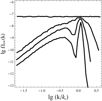
The numerically calculated power spectrum in the running mass model is shown in Fig. 5 for two sets of parameters. Parameters , of the spectra are chosen with taking into account the PBH constraints obtained in the previous work of authors [40]. It is seen from the figure, that the maximum values of the power spectrum (at large ) are very sensitive to the value of the spectral index running. The upper curve in Fig. 5 represents the spectrum with largest possible for other parameters being fixed. Larger values of spectral index running will cause too large curvature perturbation spectrum values - in this case, too many PBHs will be produced with mass g.
The spectra of second-order GWs corresponding to the scalar spectra of the running mass model are shown in Figs. 6, 7. As in the previous case of a peaked-power spectrum (Fig. 4), it is seen from these figures that scalar perturbation power spectrum generated in the running mass model can be a source of significant amount of GWs, detectable in experiments studying the frequency region Hz.
The results shown in Figs. 6, 7 correspond to different values of and (i.e., to different energy scales of inflation). It was shown in [40] that PBH constraints depend on a proposed value of : the maximum running allowed is for GeV and for GeV (for in both cases). The difference in PBH constraints originates from the connection between comoving scale and horizon mass (see Eq. 5): Mpc-1 corresponds to g, while Mpc-1 corresponds to g. PBH constraints in the region of g follow from inspection of extragalactic photon background data while PBH constraints near g follow from available limits on the intensity of extragalactic neutrino background [40].

IV Conclusions
1. The dependence of a form of the -curve on the width of the peak of the scalar power spectrum is carefully studied (Fig. 3). It is shown that this curve has a characteristic “double-peak” form; the height of the larger maximum weakly depends on the width of the proposed distribution (see Eq. (44)). It is shown also that the -function depends, in fact, on the ratio where is the position of the maximum in .
2. The distribution for the induced GWB is calculated for two different cases: for the scalar spectrum with a peak (Eq. (44)) and for the scalar power spectrum predicted by the running mass model. It is seen from the resulting figures that the behavior of -curves near the maximum in both cases is rather similar.
3. It is shown that maximum values of -distributions for the induced GWB can be constrained by PBH searches in the wide region of the comoving scales, Mpc-1 (the upper curves in Figs 4, 6, 7 are maximum ones in this sense). It is shown also that, up to now, the PBH constraints are more strong than the available limits from LIGO (see Fig. 4 and 6). In particular, it follows from Fig. 4 that the maximum value of at frequency Hz is equal to (supposing that the scalar power spectrum has the peak in this region).
Finally, it follows from Fig. 4 that, in not very distant future, when the limits for from LIGO experiment will reach the level and lower, their data will give stronger constraints on amplitudes of scalar power spectra then today’s constraints following from PBH studies. It means, that the future experiments with LIGO detector, limiting the power spectrum of primordial scalar perturbations, will give the new constraints for PBH production in the early universe. The interval of frequencies of ground-based detectors is about Hz to few kHz, and the corresponding interval of PBH masses is from to g.
In this paper we have made an accent on second-order GWs with frequencies mHz - kHz, which will be probed by space-based and ground-based laser interferometer experiments. The same effects (particularly, rather large values of induced ) can appear in other frequency regions, for which is not probed by observations (Hz), e.g., for Hz, where high-frequency GW detectors operate, or at Hz, where is constrained by pulsar timing data (in fact, these data already allow to put limits on PBH abundance [34] for PBHs with rather large masses). In the band probed by CMB measurements, the effects from second-order GWs are carefully studied in [33] and shown to be small.
Acknowledgments.
The work was supported by Federal Agency for Science and Innovation under state contract 02.740.11.5092.
References
- [1] B. Allen, “The stochastic gravity-wave background: Sources and detection”, In Les Houches 1995, Relativistic gravitation and gravitational radiation, pp. 373-417; arXiv:gr-qc/9604033.
- [2] M. Maggiore, “High-energy physics with gravitational-wave experiments”, arXiv:gr-qc/9803028.
- [3] A. Buonanno, “Gravitational waves from the early universe,”, In Boulder 2002, Particle physics and cosmology, pp. 855-892; arXiv:gr-qc/0303085.
- [4] M. Gasperini and G. Veneziano, Phys. Rept. 373, 1 (2003) [arXiv:hep-th/0207130].
- [5] L. P. Grishchuk, Sov. Phys. JETP 40, 409 (1975) [Zh. Eksp. Teor. Fiz. 67, 825 (1974)].
- [6] A. A. Starobinsky, JETP Lett. 30, 682 (1979) [Pisma Zh. Eksp. Teor. Fiz. 30, 719 (1979)].
- [7] V. A. Rubakov, M. V. Sazhin and A. V. Veryaskin, Phys. Lett. B 115, 189 (1982).
- [8] R. Fabbri and M. d. Pollock, Phys. Lett. B 125, 445 (1983).
- [9] L. F. Abbott and M. B. Wise, Nucl. Phys. B 244, 541 (1984).
- [10] A. A. Starobinsky, Sov. Astron. Lett. 11, 133 (1985).
- [11] L. M. Krauss and M. J. White, Phys. Rev. Lett. 69, 869 (1992) [arXiv:hep-ph/9205212].
- [12] D. Polarski and A. A. Starobinsky, Class. Quant. Grav. 13, 377 (1996) [arXiv:gr-qc/9504030].
- [13] M. Gasperini and G. Veneziano, Astropart. Phys. 1, 317 (1993) [arXiv:hep-th/9211021].
- [14] M. Gasperini and M. Giovannini, Phys. Rev. D 47, 1519 (1993) [arXiv:gr-qc/9211021].
- [15] V. F. Schwarztmann, JETP Letters 9, 184 (1969).
- [16] R. Brustein, M. Gasperini and G. Veneziano, Phys. Rev. D 55, 3882 (1997) [arXiv:hep-th/9604084].
- [17] M. S. Turner and F. Wilczek, Phys. Rev. Lett. 65, 3080 (1990).
- [18] A. Kosowsky, M. S. Turner and R. Watkins, Phys. Rev. D 45, 4514 (1992).
- [19] E. J. Copeland, A. R. Liddle, D. H. Lyth, E. D. Stewart and D. Wands, Phys. Rev. D 49, 6410 (1994) [arXiv:astro-ph/9401011].
- [20] S. Y. Khlebnikov and I. I. Tkachev, Phys. Rev. D 56, 653 (1997) [arXiv:hep-ph/9701423].
- [21] J. F. Dufaux, A. Bergman, G. N. Felder, L. Kofman and J. P. Uzan, Phys. Rev. D 76, 123517 (2007) [arXiv:0707.0875 [astro-ph]].
- [22] C. Grojean and G. Servant, Phys. Rev. D 75, 043507 (2007) [arXiv:hep-ph/0607107].
- [23] R. Easther, J. T. . Giblin and E. A. Lim, Phys. Rev. Lett. 99, 221301 (2007) [arXiv:astro-ph/0612294].
- [24] M. R. DePies and C. J. Hogan, Phys. Rev. D 75, 125006 (2007) [arXiv:astro-ph/0702335].
- [25] C. J. Hogan, Phys. Rev. Lett. 85, 2044 (2000) [arXiv:astro-ph/0005044].
- [26] G. S. Bisnovatyi-Kogan and V. N. Rudenko, Class. Quant. Grav. 21, 3347 (2004) [arXiv:gr-qc/0406089].
- [27] R. Anantua, R. Easther and J. T. Giblin, Phys. Rev. Lett. 103, 111303 (2009) [arXiv:0812.0825 [astro-ph]].
- [28] S. Matarrese, O. Pantano and D. Saez, Phys. Rev. Lett. 72, 320 (1994) [arXiv:astro-ph/9310036].
- [29] S. Matarrese, S. Mollerach and M. Bruni, Phys. Rev. D 58, 043504 (1998) [arXiv:astro-ph/9707278].
- [30] C. Carbone and S. Matarrese, Phys. Rev. D 71, 043508 (2005) [arXiv:astro-ph/0407611].
- [31] S. Mollerach, D. Harari and S. Matarrese, Phys. Rev. D 69, 063002 (2004) [arXiv:astro-ph/0310711].
- [32] K. N. Ananda, C. Clarkson and D. Wands, Phys. Rev. D 75, 123518 (2007) [arXiv:gr-qc/0612013].
- [33] D. Baumann, P. J. Steinhardt, K. Takahashi and K. Ichiki, Phys. Rev. D 76, 084019 (2007) [arXiv:hep-th/0703290].
- [34] R. Saito and J. Yokoyama, Phys. Rev. Lett. 102, 161101 (2009) [arXiv:0812.4339 [astro-ph]].
- [35] H. Assadullahi and D. Wands, arXiv:0907.4073 [astro-ph.CO].
- [36] E. Bugaev and P. Klimai, Phys. Rev. D 78, 063515 (2008) [arXiv:0806.4541 [astro-ph]].
- [37] E. D. Stewart, Phys. Lett. B 391, 34 (1997) [arXiv:hep-ph/9606241].
- [38] E. D. Stewart, Phys. Rev. D 56, 2019 (1997) [arXiv:hep-ph/9703232].
- [39] D. H. Lyth, K. A. Malik, M. Sasaki and I. Zaballa, JCAP 0601, 011 (2006) [arXiv:astro-ph/0510647].
- [40] E. Bugaev and P. Klimai, Phys. Rev. D 79, 103511 (2009) [arXiv:0812.4247 [astro-ph]].
- [41] B. Abbott et al. [The LIGO Scientific Collaboration & The Virgo Collaboration], Nature 460, 990 (2009).
- [42] B. Abbott et al. [LIGO Collaboration], Astrophys. J. 659, 918 (2007) [arXiv:astro-ph/0608606].
- [43] L. Covi and D. H. Lyth, Phys. Rev. D 59, 063515 (1999) [arXiv:hep-ph/9809562].
- [44] L. Covi, D. H. Lyth and L. Roszkowski, Phys. Rev. D 60, 023509 (1999) [arXiv:hep-ph/9809310].
- [45] L. Covi, Phys. Rev. D 60, 023513 (1999) [arXiv:hep-ph/9812232].
- [46] G. German, G. G. Ross and S. Sarkar, Phys. Lett. B 469, 46 (1999) [arXiv:hep-ph/9908380].
- [47] L. Covi, D. H. Lyth, A. Melchiorri and C. J. Odman, Phys. Rev. D 70, 123521 (2004) [arXiv:astro-ph/0408129].
- [48] S. M. Leach, I. J. Grivell and A. R. Liddle, Phys. Rev. D 62, 043516 (2000) [arXiv:astro-ph/0004296].
- [49] E. V. Bugaev and K. V. Konishchev, Phys. Rev. D 66 (2002) 084004 [arXiv:astro-ph/0206082].
- [50] L. Alabidi and K. Kohri, Phys. Rev. D 80, 063511 (2009) [arXiv:0906.1398 [astro-ph.CO]].
- [51] L. P. Grishchuk, Proc. of the first J. A. Wheeler School on Astrophysical Relativity, Eds. I. Ciufolini and R. Matzner, Springer (2008) [arXiv:0707.3319 [gr-qc]].
- [52] T. L. Smith, M. Kamionkowski and A. Cooray, Phys. Rev. D 78, 083525 (2008) [arXiv:0802.1530 [astro-ph]].