Direct Observation of Cosmic Strings
via their Strong Gravitational Lensing Effect:
II. Results from the HST/ACS Image Archive
Abstract
We have searched 4.5 square degrees of archival HST/ACS images for cosmic strings, identifying close pairs of similar, faint galaxies and selecting groups whose alignment is consistent with gravitational lensing by a long, straight string. We find no evidence for cosmic strings in five large-area HST treasury surveys (covering a total of 2.22 square degrees), or in any of 346 multi-filter guest observer images (1.18 square degrees). Assuming that simulations accurately predict the number of cosmic strings in the universe, this non-detection allows us to place upper limits on the unitless Universal cosmic string tension of , and cosmic string density of at the 95% confidence level (marginalising over the other parameter in each case). We find four dubious cosmic string candidates in 318 single filter guest observer images (1.08 square degrees), which we are unable to conclusively eliminate with existing data. The confirmation of any one of these candidates as cosmic strings would imply and . However, we estimate that there is at least a 92% chance that these string candidates are random alignments of galaxies. If we assume that these candidates are indeed false detections, our final limits on and fall to and . Due to the extensive sky coverage of the HST/ACS image archive, the above limits are universal. They are quite sensitive to the number of fields being searched, and could be further reduced by more than a factor of two using forthcoming HST data.
Keywords:
gravitational lensing — surveys — cosmology: observations1 Introduction
Cosmic strings, which are topological defects formed in the very early universe and persisting to the present epoch, are a quite generic prediction of many modern cosmological models (Kibble, 1976; Vilenkin & Shellard, 1994; Hindmarsh & Kibble, 1995). As microscopic objects, their internal structure can be characterised by a single number, the string tension which we express in unitless form . Numerical simulations of this phenomenon have converged on a picture where horizon-scale strings are consistently predicted to lie within the observable universe (see Polchinski, 2007, for a review). This suggests the possibility of a direct detection.
Currently, the best limits on the properties of a putative network of long strings come indirectly from studies of the CMB power spectrum and pulsar timings. The CMB power spectrum is now sufficiently well-modeled so as to permit only a very small fraction of the power in temperature fluctuations at the last scattering surface to be due to strings of any type (Pogosian et al., 2004), and Pogosian et al. (2006) sets 95% condfidence limits on of . Pulsar timing experiments like those described in Kaspi et al. (1994); Damour & Vilenkin (2005) give tighter limits, but make model-dependent assumptions on the relative densities of string loops and the long strings we search for here. Additionally, pulsar timing limits rely on string oscillations to produce gravitational radiation in observable frequency ranges (Accetta & Krauss, 1989; Mack et al., 2007). But some cosmic string models decay via Goldstone bosons or other field couplings (Polchinski, 2004b).
Direct searches for cosmic strings provide an important complement to those statistical studies. Direct searches in the CMB rely on the movement of strings, which introduce a very small apparent differential between light from other side of the string (Kibble, 2004):
| (1) |
Where is the projection of the string along the line of sight, is the angular distance from the observer to the CMB, and is the angular distance from the string to the CMB. This redshift is potentially observable using the CMB as a backlight. The instrumentation required to make these observations at high resolution is still in its infancy (Zwart et al., 2008; Muchovej et al., 2007; Stewart & Brandenberger, 2009; Fowler et al., 2007; Bouchet, 2007). Previous attempts at lower resolution have not resulted in any detections, and produced upper limits on the string tension of (Sazhina et al., 2008; Lo & Wright, 2005; Jeong & Smoot, 2007). This induced redshift is of order , too small to be detected in the optical spectroscopic galaxy surveys, where it would be dominated by galaxy motions.
Cosmic strings are also directly observable in optical imaging surveys via their gravitational lensing effect (Vilenkin, 1984; Sazhin & Khlopov, 1989, e.g.). Cosmic strings produce a unique lensing signal: two identical images of a source separated by :
| (2) |
Where is the distance between the observer and the source and is the distance between the string and the source.
In our first paper (Gasparini et al. 2008, Paper I), we showed how high resolution optical imaging surveys are capable of producing direct limits on the cosmic string tension competitive with the indirect detection from the CMB power spectrum analysis. For the tensions allowed by the CMB power spectrum analysis, this separation is ”, and the cross-section for lensing is similarly small. This realisation immediately drives us towards the need to use the most numerous distant objects—faint galaxies—as backlights, and to focus on surveys with high angular resolution.
Early optical cosmic string searches focused on large image separations and bright galaxies, but no candidate string lenses have survived inspection at higher resolution (Agol et al., 2006; Sazhin et al., 2007). Ground-based optical surveys are hampered by limited resolution and cannot probe (de Laix, 1997). Conversely, the recent searches by Christiansen et al. (2008) using the Hubble Space Telescope (HST) GOODS survey images and Timothy et al. (2009) using HST COSMOS survey images did have the angular resolution to show that no string with crossed their survey fields, but did not have the sky coverage needed to be able to place any universal limit on the string tension.
We need both large survey area and high resolution to set universal limits on string tension. For the case of HST, our best current source of high resolution imaging survey data, the solid angle needed to give a universal limit on the string tension is a few square degrees, provided this area is cut up and distributed evenly across the sky. As discussed in Paper I, a contiguous survey of comparable area would provide much weaker limits due to the clustering of cosmic string events around the roughly long strings in the sky.
In this work we search the HST/ACS archive, whose images match all three of the angular resolution, area and pointing distribution criteria, and so produce the strongest direct gravitational lensing limit on the cosmic string tension and density.
This paper is organised as follows: in Section 2, we briefly review the relevant basic theory of cosmic strings. We then discuss how searching for string lensing events can be used to set new limits (Section 3). Regarding our actual search for string lenses, we explain our use of simulated string lensing images in Section 4, and in Section 5 we describe our string-finding technique. After a brief description of the archival dataset in Section 6, we present our results in Section 7 and the corresponding limits on the string tension and density in Section 8. Finally, we discuss the implications of this work in Section 10.
2 String Lensing Theory
When searching for cosmic strings via their gravitational lensing effect, we only need to understand a few basic facts about them. We must know what type of multiple image system a cosmic string produces, and we must understand what string evolution tells us about the number of strings in the local () universe.
Cosmic strings, whether topological defects or stretched fundamental strings, can produce two identical images separated by in Eq. 2 so long as they do not “cut” the source they are lensing and so long as they are straight on scales comparable to the image separation. By “cutting” a source, we mean that the redshift-dependent strip of sky which the string copies only includes a part of a source, and the source in incompletely copied. We study this effect via simulation in Section 4.2. We discuss our assumption of straight strings below.
2.1 String network topology: straight strings and loops
We can only observe a string by its gravitational lensing effect if it crosses one of our search fields; we then expect it to be more readily detectable if it is straight on the scale of the field. We consult the theory and simulations of cosmic strings to determine whether these are reasonable possibilities. Horizon scale strings are a generic prediction of string network simulations (Polchinski, 2004a), but we must consider the total angular length of observable string and, and to what extent small scale structure (kinks and curvature) will affect the image pair alignment. We also explore the possibility of detecting string loops.
Simulations (Allen & Shellard, 1990) tend to agree that during the matter dominated epoch and beyond, the long string density is:
| (3) |
where represents the average length of long, straight string within a cosmological volume, the concentration of string. These simulations assume that strings “intercommute” with probability of 1. Lowering this probability raises the simulated value of , but we assume unity intercommutation probability, because it is theoretically favoured.
We can relate to the number of cosmic strings within some redshift limit. Substituting in for the co-moving matter density, we have:
| (4) |
We divide by (where is the angular diameter distance to the string) and obtain the concentration of string in angular units, accounting for projection effects:
| (5) |
Multiplying by the cosmological volume element and integrating over redshift yields the total expected angular length of string on the sky, in radians, :
| (6) | |||||
| (7) | |||||
corresponds to a single straight string stretching across the visible sky. Setting gives us 21 radians of string within redshift 2. This in turn corresponds to roughly 7 straight strings with redshift . Even survey fields as large as a few square degrees would most likely not be crossed by a string, and would therefore have no chance of seeing a long string regardless of survey depth or resolution (see Section 3.1 for details). A survey of the same area comprising a large number of smaller, well-distributed fields stands a much better chance of “hitting” a string.
Even if a string crosses one of our search fields, detecting it may be nontrivial. Cosmic strings that are straight on scales comparable to the field size should be readily identifiable: groups of aligned galaxy pairs make good candidates for being multiple image systems generated by the string. Fields of arcmin would then result in the requirement that, for it to be detectable, a cosmic string be straight on Mpc scales.
What can we infer from the string network simulations about the likely straightness of horizon-scale strings? Suppose that cosmic strings follow random walks. The total length of a string within the horizon of a string undergoing a random walk is roughly where is the horizon scale and is the characteristic length of the random walk. Assuming a string tension , the random walk length, and similarly the radius of curvature of the string, must be of order the or would quickly exceed 60 and would be large enough to affect the CMB spectrum (see Section 3). So must be large and this random walk behaviour only affects the Mpc scale perturbatively. The simulations do show that a string’s self-interactions and its interactions with other strings can induce smaller scale “cusps” which propagate along the string. However, at least some models suggest that these cusps will leave strings that are essentially straight on Mpc scales (Rocha, 2008).
String evolution networks also produce loops. Loops smaller than a few Mpc would not be detectable as simple alignments of image pairs. Mack et al. (2007) provides a framework for detecting string loops with proposed high resolution radio surveys. Many models and simulations set the scale of cosmic loops (Caldwell & Allen, 1992) to be of order the horizon scale, and so it is possible that many cosmic string loops are straight on the Mpc scale, but we do not include them when marginalising over string concentration in our calculations.
2.2 String lens observability
In this section we summarise the various observable features of cosmic string lenses, and thus motivate our particular search strategy.
We might hope to detect a cosmic string using a single, obvious string lensing event, where the images are demonstrably translated copies of each other (see Agol et al., 2006, for such an analysis). It is only possible to determine if a single pair is the result of string lensing if the pair separation is several times larger than the PSF, and if the sources are bright and well-resolved. The large separation requirement would directly limit our ability to probe the small (subarcsecond) string tensions of interest. The bright source requirement, and the fact that there are exponentially fewer bright sources than dim sources, would limit our ability to probe small .
The key observable feature of a cosmic string is therefore that it produces many pairs of images, as it cuts across many background sources (Huterer & Vachaspati, 2003; Oguri & Takahashi, 2005). We could look for local overdensities of well-matched (in magnitude, ellipticity and orientation) pairs, as is expected to occur when a kinked or coiled string lies in the field. This is the approach taken by Christiansen et al. (2008), and only works when the number of string pairs () is large enough that string lensing can be detected against the very high background of pairs described by the small-scale correlation function.
However, on arcsecond and sub-arcsecond scales the background sources are highly correlated (Morganson & Blandford, 2008). The increase in the abundance of apparent galaxy pairs due to the presence of a cosmic string is, as we shall see, quite small. Only for the expected straight strings from the previous section do we expect a measurable phenomenon: the appearance of groups of apparent galaxy pairs aligned with each other.
The similarity of the members of each aligned pair should still be a useful indication of string lensing. At image separations of , we are probing down to the scale of the source size itself, and so many multiple image systems will contain incompletely copied sources. If these images were well-resolved, we could detect a sharp edge, but small, incompletely copied sources look unremarkable. Pairs with incomplete images can, in rare cases, have significant differences in their magnitudes and ellipticities. In Section 4.2, we quantify these differences.
3 Estimating the expected number of string detection
In order to set limits on string parameters, we calculate the expected number of string detections in a given dataset, .
Each (assumed rectangular) field is defined by three parameters, two spatial extents and , and its limiting magnitude, . A given string is defined by its tension, , its inclination along the line of sight, , and its redshift, . The intersection between the string and the field is defined by , the projected angular length of string that crosses the field.
To calculate , we must first calculate the probability that a randomly oriented string crosses a field with crossing length , . We then calculate the probability that a string which crosses our field with length is detected, . Knowing these two quantities, we can integrate over all possible strings to obtain for a randomly oriented field:
| (8) | |||||
In Section 3.3 below, we discuss how we transform our expression for the probability of a detection in a single field to our 95% detection limits for a multi-field survey.
3.1 The Probability of a String Crossing a Field
We define as the probability that a string at redshift will cross our field with length at inclination angle, , to the line of sight. We assume that our fields are much smaller than a radian and that our strings are straight on scales longer than a few arcminutes (the size of a single field). We break down the probability of a string crossing our field with overlap length into two terms: the probability of the field crossing a randomly oriented line that is 1 radian long and the projected length of string at redshift (in radians):
| (9) |
is a quantity derived solely from two dimensional spherical geometry without any cosmological input. It is the probability of a randomly positioned rectangle being crossed by a randomly oriented rad arc with an overlap length of . The angular length 1 radian is arbitrary and chosen for mathematical convenience. We provide its (somewhat cumbersome) geometrical derivation in the appendix.
The remaining terms represent the expected projected angular length of string on the sky at every redshift and the cosmological volume element. If we plug in our model value of (equation 3) and the volume element, we obtain:
| (10) |
3.2 The Probability of a String Crossing being observable
Assuming that a string crosses a field with overlap , we define the probability of that string producing a detectable lensing signature as . To obtain this function, we must calculate the expected number events for our string and field. This is just a (-dependent) lensed area times a (-dependent) source density, integrated over .
The lensing cross sectional area of a string is its length, , times the string lensing width in equation 2:
| (11) |
We model the source density, , using the redshift distribution distribution from Leauthaud et al. (2007) and a fit to the magnitude distribution of COSMOS:
| (12) | |||||
This equation assumes magnitudes observed in the F814W filter. For fields imaged in a different filter, we measure the source density and assume the F814W limiting magnitude that would yield an identical density.
We multiply the cross sectional area by the (redshift-dependent) density of sources and integrate over source redshift to obtain the expected number of lensing events
| (13) |
Here, is the minimum source redshift that will produce a resolvable lensing event:
| (14) |
is the “effective resolution,” or the angular separation at which actual faint pairs in our survey can realistically be deblended. Morganson & Blandford (2008) found ”, and we use this value when deriving detection limits.
Most of our events will involve faint sources that are fairly weakly clustered on arcminute scales, so we can assume a Poisson event rate. We require three aligned pairs of similar galaxy images to claim a string detection, so we calculate the probability of making three detections or more:
| (15) |
When probing a potential string detection, we incorporate the information we get from the detection into the above analysis. The expected number of lensing events becomes
| (16) |
Where, and are the observed source redshifts that will produce the minimum and maximum observed lensing separations:
| (17) | |||||
In addition, we define to include the observed number of detected pairs:
| (18) |
3.3 Expected number of string detections and string limits in a multifield survey
In this paper we aim to set limits on using multifield surveys, and as an intermediate step, we must calculate , the expected number of string detections across our complete dataset. must be calculated numerically for every field at each tension , but it is linearly proportional to . For each field, we calculate , and then compute .
The expected number of string detections of multiple fields will add linearly so long as the fields are randomly distributed, so we have:
| (19) | |||||
To see what and give us 95% chance of detecting a string, we assume a Poisson distribution for the number of detections. A random variable taken from a Poisson distribution with a mean of only has a 5% chance of being 0. So for a given , we set:
| (20) | |||||
| (21) |
To compute proper Bayesian confidence limits, we must must assume prior distributions for and . We assume is log-uniformly distributed between and , and we take a logarithmic version the distribution from Eq. 3:
| (22) | |||||
The probability of a null detection is and the probability of observing a detection in one field and no detections in all other fields is . We use the above priors, these formulae and a standard Bayesian formulation to produce confidence limits in Section 8.
4 Simulated Images
As we discussed in Paper I and Section 2 above, to detect a cosmic string lensing event one must be able to detect close pairs of faint objects. Developing and testing search algorithms, and then characterising their respective selection functions, requires sets of simulated images in which we know the location of the sources and the strings. These mock images are based on those used in the faint source correlation function measurement by Morganson & Blandford (2008). These simulations reproduce the magnitude, area and ellipticity distributions of the faintest galaxies in HST/ACS GOODS images; we adapt them for cosmological settings with cosmic strings by including magnitude-dependent clustering, stochastic redshift assignment and a string lensing effect. We provide a very brief outline of the image simulation procedure we use in this section, and refer the reader to the paper by Morganson & Blandford (2008) for more details.
4.1 Image Production
Our standard simulated images are square, consisting of pixels. Each pixel is a ” square, so our mock frames are ” on a side. In each mock image we place a single straight string (as described in Section 4.1), with known orientation. We use these images to test our string detection algorithms and to measure the detection probability. We also produce a set of narrow ”” images, each containing a single string, in order to produce a high density of multiply-imaged faint galaxies and allow us to quantify the string lensing effect on the galaxy images themselves (see Section 4.2).
We choose source redshifts and magnitudes using the distributions in equation 12. Each source is assigned an independent redshift, based solely on its magnitude, and printed into the image with the nearest discrete (0.1, 0.3, 0.6, 1, 1.5, 2, 2.5, 3, 3.5, 4, 5, 6). We have one string per image. The strings are located at a constant redshift (the analog of the thin lens approximation). Each image is lensed by copying and shifting half of the image by the amount given equation 2. All simulated strings are absolutely straight and vertical. We add the images at each to produce an image with all sources.
Finally, we convolve the lensed and combined images with a point spread function (PSF) determined by an average of many model PSFs calculated using the “Tiny Tim” software package.
We then add a noise background which has been convolved with a separate PSF that mimics the image combination process. We vary the noise amplitude to produce images of various desired limiting magnitudes.


In Fig. 1, we show 5 examples of typical string-lensed image pairs from one of our simulated fields. Overlaid are ellipses representing the orientation and ellipticity measured for each source using the SExtractor program (Bertin & Arnouts, 1996). We see that some pairs will have well-measured and well-matched magnitude, size, ellipticity and orientation, and that these should be closely-matched between conjugate images in the multiple-image system. However, due to the prevalence of faint, poorly-measured sources, and to strings splitting sources, most pairs are not as readily recognizable as string lensed pairs. We quantify this below.
4.2 Properties of simulated string-lensed objects
One important application of our simulations is to compare the statistical properties of string lens multiple-images with those of unlensed, background galaxy pairs. An idealised string lensing event would produce two identical galaxy images, but incomplete copying of sources leads to non-ideal string-lensing. Still, as we show in this section, string-lensed pairs tend to be more similar than random pairs.
We compare catalogs of string-lensed image pairs and unlensed close galaxy pairs generated from a large number of simulated images. These images are the long, narrow strips mentioned in Section 4. We made a set of thin (””) simulated images with a string running along the long axis. For each combination of lens redshift (0.1, 0.5, 1, 1.5, 2, 3), (0.3”, 0.4”, 0.5”, 1”, 2”) and the F606W-band AB limiting magnitude (25, 26, 27, 28), we made 100 images, for a total of 120000.
In each image, we identify the string-lensed pairs as those whose centre lies within of the string, and whose separation vector is of length and within 0.05 radians of being perpendicular to the straight, simulated string. For the brightest magnitude limit, , this latter condition is relaxed to 0.1 radians, because the bright, large sources have larger uncertainty in their positions. In all we generate 30000 simulated string-lensed image pairs.
Those sources whose centre is further than from the string and whose separation is are chosen as sample background pairs, regardless of orientation. We find 500000 such background pairs.
We divide our catalogs of string pairs and background pairs along three different axes. First, we split the data into different limiting magnitude bins (25, 26, 27, 28). The fainter our limiting magnitude, the smaller the sources we tend to detect. We then further divided the pairs into two classes of separation of the string pair, “close” and “far,” with ” (a characteristic source size) being the cutoff separation. Pairs separated by distances much larger than this threshold are well-resolved and deblended, and so should be more similar than close pairs. Finally, we divide our sources into two classes: “dim” sources that are within one magnitude of the limit, and “bright” sources that are more than one magnitude above the limiting magnitude. Bright sources tend to have more distinct morphology which allows us to distinguish lensed pairs from random pairs more easily.
We quantify the similarity between sources in pairs using three parameters. The first two are the measured magnitude difference between the sources in a pair,
| (23) |
and the pseudo-vector ellipticity dot product,
| (24) |
where is the SExtractor ellipticity of the source, and is its orientation.
We also use , the angle between the pair separation vector and a line perpendicular to the string, to determine how well-aligned a string pair is with its string candidate. Note that two well-resolved, well-separated and well-measured string-lensed conjugate images will have , , and .


The distributions of these three parameters are shown in Fig. 2. We fit these distributions with the following functions:
| (25) | |||||
| (26) | |||||
| (27) | |||||
| (28) |
We measure separate , and for string pairs and background pairs; is the maximum we accept (0.05 or 0.1 rad, depending on ). The resulting model distributions are overlaid on Fig. 2, and the fit parameters tabulated in Table 1.
In this table we can see that sources in string pairs have lower average and higher than random pairs. We also see that for string pairs is strongly clustered within . Random pairs have a uniform random and their distribution is not shown. In Fig. 2 we see that our model distributions give good fits in all cases. We use these models in the computation of string detection probability in Section 5.4.
| Limiting Magnitude | Subsample | |||||||
|---|---|---|---|---|---|---|---|---|
| 25 | Close, Bright | 0.350 | 0.604 | 0.086 | 0.006 | 0.095 | 0.109 | 0.046 |
| Close, Faint | 0.355 | 0.511 | 0.010 | 0.010 | 0.126 | 0.152 | 0.052 | |
| Far, Bright | 0.327 | 0.997 | 0.057 | 0.002 | 0.154 | 0.157 | 0.036 | |
| Far, Faint | 0.382 | 0.569 | 0.016 | 0.000 | 0.134 | 0.157 | 0.044 | |
| 26 | Close, Bright | 0.215 | 0.707 | 0.081 | 0.019 | 0.131 | 0.126 | 0.026 |
| Close, Faint | 0.284 | 0.534 | 0.041 | 0.013 | 0.111 | 0.153 | 0.028 | |
| Far, Bright | 0.285 | 0.907 | 0.069 | 0.004 | 0.121 | 0.129 | 0.021 | |
| Far, Faint | 0.324 | 0.633 | 0.020 | 0.001 | 0.125 | 0.153 | 0.023 | |
| 27 | Close, Bright | 0.205 | 0.666 | 0.086 | 0.026 | 0.122 | 0.145 | 0.023 |
| Close, Faint | 0.234 | 0.530 | 0.039 | 0.014 | 0.101 | 0.159 | 0.027 | |
| Far, Bright | 0.299 | 0.942 | 0.090 | 0.000 | 0.125 | 0.141 | 0.019 | |
| Far, Faint | 0.263 | 0.651 | 0.033 | 0.001 | 0.115 | 0.150 | 0.021 | |
| 28 | Close, Bright | 0.200 | 0.684 | 0.100 | 0.023 | 0.116 | 0.138 | 0.022 |
| Close, Faint | 0.233 | 0.545 | 0.039 | 0.015 | 0.093 | 0.158 | 0.026 | |
| Far, Bright | 0.259 | 0.991 | 0.113 | 0.009 | 0.138 | 0.144 | 0.018 | |
| Far, Faint | 0.249 | 0.668 | 0.038 | 0.004 | 0.109 | 0.147 | 0.020 |
Incidentally, the term in equation 27 represents the background pairs which are uniformly distributed in . We use it to find that there is no more than background pair contamination in any of the string pair subsamples.
5 Lens-finding Methodology
As explained in Section 2, we look for strings that are straight on scales at least as large as ’ (corresponding to Mpc at ) by correlating close pairs of faint sources along straight lines across small-field images. We give a brief summary of the search methodology, before describing it in more detail.
5.1 Summary
For each field, we first create a catalog optimised to contain as many faint sources as possible, deblending close pairs aggressively. From this we produce a catalog of close (”) pairs of objects. The line which bisects each pair is then parametrised by its position and orientation in the image — this line represents a putative cosmic string. The change of variables between image pair position and orientation to bisector line parameters is a modified “Hough transform:” pairs straddling the same straight line will appear very close together in the Hough space (Ballester, 1996). We therefore identify clusters of points in the Hough space as indicators of possible strings. We then assign a score to each string candidates by evaluating the similarity of constituent pairs and their alignment with the possible string. We visually inspect high-scoring candidate strings, remove non-physical image pairs and retest them against a higher threshold. In the next two subsections we explain this process in more detail.
5.2 Image pair detection
We aim to find many sources and not to exclude pairs. We achieve both these goals by emulating the catalog production techniques in Morganson & Blandford (2008) which are in turn influenced by Benitez et al. (2003). Roughly speaking, we used the SExtractor program (Bertin & Arnouts, 1996) to produce catalogs of faint sources. After we make an initial source catalog, we find all pairs separated by less than ” and make a catalog of pairs. We do not probe above 5” because this corresponds to a minimum and a typical (including projection and redshift effects) which is not an interesting area of parameter space, because it is ruled out with high significance by Jeong & Smoot (2007).
Our source extraction parameters are summarised in Table 2. We make three changes to the setup used by Morganson & Blandford (2008). To make our faint detections very sensitive, we lowered our DETECT_THRESH from to for WEIGHT type weight images. However, we primarily use RMS weight images (which were not available for the GOODS data that our catalog techniques were initially designed for), and the two types are normalised differently. Setting the DETECT_THRESH for RMS weight images to produces roughly identical catalogs as those produced above with weight type WEIGHT. We also changed DEBLEND_MINCONT from to to promote more aggressive deblending.
These changes do not produce many false counts from noise peaks in our catalogs. Running SExtractor on “negative” images where the pixels have been multiplied by produces false sources for every source detected in real images. However, complex sources are often deblended into several sources. At this stage, the catalogs are inclusive as possible; false pairs will be rejected later in the lens-finding process.
| WEIGHT_TYPE | MAP_RMS |
|---|---|
| Filtering FWHM (Pixels) | 1.5 |
| DETECT_THRESH | 0.895 |
| DETECT_MINAREA | 10 |
| DEBLEND_NTHRESH | 32 |
| DEBLEND_MINCONT | 0.0003 |
From our initial faint source catalog, we produce a catalog of close pairs. In this catalog, we derive various pair parameters including the centre of each pair, , and the separation vector . We also compute each pair’s , and parameters (see Section 4.2) and interpolate between limiting magnitudes to obtain the statistical properties of string pairs and background pairs in Table 1.
String-lensed image separations can be , so we never set a minimum when looking for string pairs. However, the number of background pairs increases with the separation limit, so we search for strings with different maximum to reduce background pairs when searching for small separation strings. We produce 15 pair subcatalogs for each field with arcsec. All the work in Section 5.3 and beyond is performed on each pair subcatalog separately.
5.3 The Modified Hough Transform to String Parameter Space
We cannot make a detailed analysis of every possible string orientation in every field and must focus on straight lines with many string lens candidates along them. An efficient way to find significant numbers of aligned pairs is to perform a suitable modified Hough transform on all detected pairs, and then accumulate a Hough space image (histogram) and search this image for significant peaks. These peaks represent multiple image pairs which could have all been lensed by the same straight string.
To convert a single image pair to its corresponding putative lensing string, we find the straight line which bisects the separation vector between the objects in the pair. For a pair at mean position and separation vector , this line is defined as:
| (29) | |||||
| (30) |
where are the coordinates of the point where the bisector line (string) comes closest to the origin (the centre of the field). We convert the impact parameter vector to polar coordinates , because a set of randomly oriented and distributed pairs will produce a uniform random field in these coordinates. is then the minimum distance (in arcsec) from the bisector line to the origin, while is the polar angle to the point of closest approach between the string candidate and the origin. is measured anticlockwise from the horizontal image axis. We illustrate this transformation graphically in Fig. 3. This transform is equivalent to a standard Hough transform of point sources, except that each pair, in addition to having a position in image space, also has an implied orientation angle. When transformed into Hough space, each of these pairs becomes a point source representing a single line which goes through a source point rather than an extended Hough source representing every line that goes through that source.

In this new mathematical space, each image pair corresponds to a single source. We would like to weight these sources by their likelihood of being a string pair rather than a background pair. To this end, we assign each source a non-unit intensity given by:
| (31) | |||||
| (32) | |||||
(Note that we approximate , since and E are uncorrelated for all but the brightest, most completely copied pairs). By construction, all pairs bisected by the same line will appear at the same point in Hough space. If for every pair, each pair would have intensity of 1 and the total Hough space flux of a feature (string) would be the number of pairs along a string. However, pairs of similar sources where are weighted more significantly than other pairs. The parameter , and we discuss its purpose and optimisation in Section 5.4.
After accumulating individual points in Hough space, and assigning them intensities, we convolve the resulting space image by a kernel so that nearby points blend together to make multi-pair Hough sources. Four degrees is the typical between the pair separation vector and the actual direction of the string. ” is the typical error in caused by projecting the string back towards the origin incorrectly due to . The resulting convolved images contain bright sources corresponding to lines in the real space images which have many pairs along them; an example is shown in Fig. 4. We extract bright sources from these images using SExtractor with DETECT_MINAREA = 7 and DETECT_THRESH = 0.16. These settings are optimised to find objects with total Hough space flux of 2 units (indicating 2 or more pairs of well-matched galaxy images lying along a line in real space). Every peak we detect in this Hough space becomes a string candidate.

5.4 Candidate Assessment: Scoring Potential Strings and Score Thresholds
Having eliminated the vast majority of possible string orientations and identifying likely string candidates as significant peaks in the Hough space image, we examine each candidate more carefully using information from each galaxy image pair to assign it a score based on its relative likelihood of it being a string lensed pair and a random pair. Our first step is to find all pairs which could possibly be associated with our string candidate. We cast a wide net finding all pairs with and within and ” of our ideal strings. This allows even very incompletely copied pairs to be included for consideration as string lensing candidate pairs.
We then maximise a string “score” defined as:
| (33) | |||||
| (34) | |||||
| (35) | |||||
Except for and , the terms in the above equation are discussed in Section 4.2 and 5.3 and represent statistical distributions of string pairs and background pairs. is the distance of the centre of the pair from the string. To simplify the calculation of , we rotate our coordinates by so that the string angle and each pair angle . All the ’s are small enough to permit linear approximations. After this rotation, is the distance of the pair along the string, is the -intercept of the string and is the of the centre of each pair from the potential string.
In parameterising our string, we only maximise with respect to and . All but the last two terms of Eq. 35 are constant, and our score is maximised by solving:
At this point, the pair with the most negative — corresponding to a much higher likelihood of being a background pair than a lensed pair — is rejected, and and are recalculated until all pairs have . Only strings with at least three positively scored pairs are considered possible strings. This three pair requirement is included in our analysis in Section 3.
Two terms in this algorithm, and are not taken directly from comparisons of simulated string pairs and background pairs. In defining we aim to penalize strings which are farther from the proposed string than could be allowed by the pair separation, its small uncertainty in position or a slight curvature of the string. The centroid of legitimate string pairs can be up to (where is the pair separation) away from the string. The angular size of a typical faint galaxy is roughly ” and this leads to a similarly sized uncertainty in position when a galaxy image is cut by a string. The radius of curvature of a horizon-scale cosmic string should be of order 1 Gpc 2.1.
Across a typical Mpc GO field, a string with a 1 Gpc radius of curvature will bend 2 kpc or an observed ” from being a straight line. We do not want to penalize strings for being less than ” or half their pair separation from the string. We therefore set .
The parameter determines the relative weighting between the existence of a pair along a string, and the degree to which the pair resembles an ideal string pair. We derive the optimal value of from our simulations. Our goal is to produce the highest score differential between the string pair and the highest scored background pair. We vary in increments of and run our algorithm on 15 simulations with limiting magnitude 27, a string at and at string tensions of (five each). produces the highest average .
Having defined a metric, S, to evaluate string candidates, we use simulated string scores to set a threshold score for all potential strings. This score will be dependent on the limiting magnitude, maximum pair separation and field size (although in practice, the field size is fairly constant). We combine these factors into , the expected score for a randomly oriented string in our field:
| (44) |
Where the term accounts for the number of resolvable strings (the number of PSF areas that fit in our Hough space). and we are summing over all the pairs separated by some which has fifteen values for each field as described in Section 5.2. We plot the observed scores of all simulated strings with three or more pairs versus the expected score in Fig. 5 and determine an empirical threshold which accepts 99.5% of simulated strings:
| (45) |

Scores will be modified slightly in Section 5.5 after string candidates have been inspected by eye and bad pairs removed, so at this point, we pass all pairs with:
| (46) |
We learned by trial that random alignments of two pairs are too common to consider as strings, so we also require that each potential string have three or more constituent pairs (three pairs detections are assumed when we use our results to set limits).
5.5 Candidate Assessment: Initial Human Inspection
String candidates which exceed the threshold in equation 46 are passed along to more detailed statistical analysis, but first the constituent pairs of each string are evaluated by eye to exclude false pairs from future consideration. The false pairs we exclude come in four types: residual cosmic rays, diffraction spikes, large foreground objects (technically not false pairs, but generally not cosmologically distant) and misprocessed data. We show examples of each in Fig. 6. A common problem with these false pairs is that they can produce an overdensities along straight lines, thus mimicking the cosmic string signal. Strings with false pairs are not automatically eliminated at this stage unless their total number of valid pairs goes below three.


5.6 Candidate Assessment: Detailed String Analysis
Having eliminated bad pairs from the potential stings, we can execute two more rigorous cuts knowing that our results will not be significantly influenced by false pairs. The first cut is to require that the string go between each pair (or nearly so) while allowing for some string curvature. The second cut is to require that the score per pair is similar to that observed in simulation.
To fit a curved string to a set of pairs, we first fit a straight line using Eq. 5.4. We then rotate the pairs by so that they are perpendicular to this fitted line. We define a Cartesian system in which is along the linear approximation of a string candidate and is perpendicular to that line. We fit the pair positions with:
| (47) |
We intentionally do not fit the curve with three degrees of freedom at once. The spatial terms are centered so that is in the middle of the string. Fitting the quadratic term in equation 47 allows for symmetric curvature across the field, as we would expect for a string with a very large radius of curvature. A full three-term quadratic fit has the undesirable property of allowing the fit to curve out sharply at either end.
As noted in Section 2.1, the curvature of the string is believed to be small. We quantify this by assigning the following Gaussian prior on :
| (48) |
The most probable curved string given the data is then given by:
Once this fit is obtained, we examine all pairs in the field that this curve does not pass through and whose closest source is more than ” away from the curve. The pair whose closest source is farthest from the curve is excluded. The fit is recalculated, first as a line and then as a curve until all pairs are either split by the curve or within ” of being split by the curve. This more strict filtering eliminates many high separation string candidates, but does not affect a significant number of simulated straight strings.
Our final method of string candidate rejection is to assert a cutoff on string score as a function of the number of pairs associated with the string, . In Fig. 7, we plot for our simulated strings and find that
| (57) |
is a threshold that accepts more than 99.5% of strings with 3 or more observed pairs.

String candidates that survive these two cuts are passed along to a final round of field-dependent inspection in which neighboring fields in surveys and multi-band images are used (where possible) to eliminate string candidates. These methods require more human involvement and are not generally applicable, so we present them separately in Section 7. Having outlined the end-to-end string candidate generation procedure, we next describe the imaging dataset we use in our string search.
6 Survey data: the HST/ACS archive
We now describe the input data for our cosmic string search. As previously discussed, we use HST optical imaging data for its high resolution and background source density. For ease and homogeneity of processing we focus on images taken with the Advanced Camera for Surveys(ACS). The total sky area imaged with ACS is approximately 12 square degrees. However, we require the images to be sufficiently deep and high galactic latitude to be able to detect significant numbers of faint galaxies at redshift 1–2, and for those images to be largely free from confusing cosmic rays. We selected 4.5 square degrees of ACS imaging data that met these criteria (although see Section 6.2 below for further discussion of cosmic ray contamination); about half of this data comes from the large programs GEMS (Rix et al., 2004), GOODS (Giavalisco et al., 2004), AEGIS (Davis et al., 2007) and COSMOS (Scoville et al., 2007). The remainder are data from extragalactic Guest Observer (GO) observations. For reasons explained in Section 7 we divide the GO images into GO-M (fields with imaging in multiple filters) and GO-S (single filter fields). Approximately 0.75 square degrees of the GO-M imaging had more than 2000 seconds exposure time, and was made public before November 2005: this subset was searched for galaxy-scale strong gravitational lenses by Marshall et al. (in preparation) as part of the HST Archive Galaxy-scale Gravitational Lens Search (HAGGLeS). Here, we use a larger set that includes more recently-observed fields, fields that were only observed in one filter and fields with a little as 1500 seconds exposure time. We retain the need for 3 exposures per field for effective cosmic ray rejection. We summarise the HST/ACS imaging data used in Table 3.
| Survey | No. of fields | Area | Mean depth | |
|---|---|---|---|---|
| (deg2) | (AB mag) | |||
| GO-S | 318a | 1.08 | 25.8 | |
| GO-M | 346a | 1.18 | 26.3 | |
| COSMOS | 575 | 1.84b | 26.5 | |
| AEGIS | 63 | 0.20 | 25.8 | |
| GEMS | 63c | 0.18 | 25.3 | |
| GOODS | 35 | 0.10 | 28.6 | |
| Overall: | 1400 | 4.48 | 26.2 |

The geometry of the GO survey is shown in Fig. 8. The avoidance of the galactic plane area can be seen, but otherwise the HST/ACS archive does a reasonable job of uniformly sampling the sky.
6.1 Survey field depths and areas
We initially search through individual fields from large surveys as though they were independent entities. When determining the limits implied by null detections in each survey, however, we view each contiguous survey as one large area (with GOODS North and GOODS South being two areas). This method automatically accounts for field overlap in surveys, reducing areas by 4% (Scoville et al., 2007, as appropriate for the largest survey, COSMOS,). We could search for strings across full surveys as though they were individual fields, but our measurement of becomes less accurate as fields get larger. In Section 7.1, we discuss how we use the contiguous nature of large surveys to eliminate string candidates. The GO fields are predominantly single ACS pointings, although in some cases we mosaiced overlapping fields together.
Very few instances of GO field overlap remain. We account for overlaps between the large program fields by working with a single catalog of unique sources for each large program area; we then correct the large program survey areas downwards by 4% (Scoville et al., 2007, as appropriate for the largest survey, COSMOS) when computing string densities and parameter constraints.

The “depth” of each field is a label allowing the sensitivities to source detection to be quantified in each field. It is defined as the F814W AB 5-sigma limiting magnitude for an extended source measured within a 0.4” radius circle, were it a faint blue galaxy at redshift 1.5. This definition was adopted to allow comparisons between fields observed in different filters: specifically we assume the Scd template spectral energy distribution of (Coleman et al., 1980) for the transformations. The depths we derive match well the extended source F814W AB limiting magnitudes calculated by the AEGIS project team (Davis et al., 2007) and the 90% faint galaxy completeness limit estimated for their images by the COSMOS team (Leauthaud et al., 2007). We chose the F814W filter for consistency with the model redshift distribution of (Leauthaud et al., 2007) that we have adopted. This is plotted for each of the surveys in Fig. 9.
6.2 Image processing and Cosmic Ray rejection
In the case of the large programs, we used the high level archive science product images provided by the project teams. The GO images were reprocessed from the uncalibrated data using the multidrizzle pipeline developed for the HAGGLeS project (Marshall et al. in preparation). This processing included a visual inspection step to remove cosmic ray clusters, satellite trails, scattered light and other confusing artifacts.
Many of the GO fields were produced from only a few raw images. While HAGGLeS aims to produce uniformly high-quality data, many fields suffer from cosmic ray corruption not recorded in the weight image. Since we are not interested in perfectly accurate catalogs but rather rare, high-level correlations, we use a simple method to extract the vast majority of these sources and accept some impurity.
We have many processed images with false sources caused by cosmic rays. Typically, these detections are around the edges of images where the input raw images did not overlap, but in some fields, cosmic rays corrupt the image interior as well. The HAGGLeS weight images usually mark these pixels as having high variance, but this process is likely to fail when there are fewer input exposures. Fortunately, cosmic ray events tend to deposit more energy on a pixel than all but the bright sources. Examining the intensity of the brightest pixel in every detect source in a typical HAGGLeS GO field produces a double Gaussian distribution as shown in Fig. 10.

The higher intensity peak is due to cosmic rays, while the lower intensity peak is due to astronomical sources. We fit the distribution with two Gaussians centered at and and with widths and , and reject sources with where:
| (58) | |||||
We do not filter out bright sources if the peaks cannot be resolved at the level. Generally, these fields have very low cosmic rays counts, but some fields are dominated by cosmic rays and were excluded during visual inspection. After we have identified a population of cosmic rays, we search for significant overdensities around the edges of our image and remove these edges if an overdensity exists. This filtering is imperfect since the cosmic ray intensity peak has a long negative tail and the source peak intensity has a long positive tail, but we estimate roughly 95% purity in typical samples. We eliminated 74 of the 738 GO fields as being unsuitable for string detection due to excessive cosmic rays, stars or foreground clusters (which prohibit string detection just like excess cosmic rays) in this way.
7 Results
The search methods described in Section 5 are successful at greatly reducing the number of potential strings in our surveys, but we must address the small number of remaining candidates in a rigorous way in order to produce detections or robust upper limits on string tension and concentration. Our methods sort through millions of possible strings in 1400 fields, leaving only 50 string candidates which we must study in more depth. These remaining candidates show every indication of being the statistical tail of coincident alignments.
In Table 4, we show how many string candidates existed at each stage of our analysis. Each of our fifteen Hough images can resolve roughly 1000 strings, so we are in effect examining 15000 potential strings per field. Only 1638 potential strings (1.2 per field) pass initial automated inspection described in Section 5.4. These candidates were all examined by eye and had any obvious bad pairs removed. Only 50 of the remaining candidates passed the final automated test in Section 5.6 with at least 3 pairs and a score per pair consistent with simulated strings. The 3-pair requirement is particularly effective at eliminating potential strings in bright limiting magnitude fields (AB Mag 26) and small separation strings, because there are fewer background pairs in these cases. Potential strings in high limiting magnitude fields (AB Mag 27), and those that produce high angular separations, have higher thresholds which require more chance alignments, and so are also efficiently excluded. It is the fields with intermediate limiting magnitudes (26 AB Mag 27) that produce the most automatically-assessed candidates, and we have relatively few candidates remaining from the GO survey (which has many shallow and deep fields) and none from GOODS (which is uniformly deep).
| Survey | Number of Fields | Resolvable Strings | Passed Assessment 1 | Passed Assessment 2 | Possible Strings |
|---|---|---|---|---|---|
| GO-Sa | 318 | 4.6 106 | 323 | 4 | 4 |
| GO-Mb | 346 | 5.3 106 | 382 | 8 | 0 |
| COSMOS | 575 | 8.7 106 | 631 | 31 | 0 |
| GEMS | 63 | 1.0 106 | 135 | 5 | 0 |
| AEGIS | 63 | 1.0 106 | 120 | 2 | 0 |
| GOODS | 35c | 0.3 106 | 46 | 0 | 0 |
| Total | 1400 | 21.9 106 | 1637 | 50 | 4 |
The numbers of pairs in the 50 remaining string candidates suggest that they are false detections. While we probe separations in the range ””, we only find candidates with maximum separations of ” or greater. If a string were making ” separated image pairs of high redshift sources, we would expect it to make roughly:
| (59) |
Where the factor is to account for the fraction of sources which are significantly behind the string, ” and 5000 are typical ACS width and the number of sources in a panel of our shallow surveys, respectively. The majority of our string candidates exhibit larger separations, indicating that we would expect even more than 7 pairs. But of our 50 string candidates, 38 consist of 3 pairs, 11 consist of 4 pairs and 1 consists of 5 pairs.
The above argument is not quantitative enough to explicitly figure into our analysis. But we can use other objective methods to show that string candidates in large surveys and fields imaged in multiple filters do not represent real cosmic strings.
7.1 Detailed string candidate inspection
The 50 candidate strings described above were selected by geometry and single filter image pair morphology alone. To test the string lens hypothesis further in each case we use different methods depending on whether the string candidate in question is in a large survey or an isolated field, and whether it has been imaged with multiple filters or just one. After all string candidates are examined, we can eliminate all but four candidates using objective criteria, and we believe that even these final four candidates could be eliminated with more data as we discuss in Section 7.2.
In large contiguous surveys, our assumption of long, straight strings requires that any strings detected in a single field be detected as collinear strings in neighbouring fields. We illustrate this idea for COSMOS in Fig. 11 by plotting the extrapolation of every string candidate into the rest of the survey. While there are some coincidentally aligned strings, there is no pattern of strongly collinear string candidates to indicate a real cosmic string. To make this analysis more precise, we use the techniques in Section 5.3 to make a single survey-wide Hough image of every string candidate in the survey (Fig. 12) and see if there are any significant alignments. Our measurements of string candidate orientation angle are precise to radians in a field, but we want to allow for modest curvature so we look for pairs whose are within of each other and whose are within (allowing the uncertainty in to be projected across the survey). Only one pair of string candidates survives this cut. This pair is composed of two candidates in acs_100036+0205_unrot, which are actually parallel but separated by more than an arcminute, rather than being collinear. Analogous Hough space images for GEMS and AEGIS also show no alignment of string candidates.
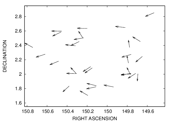

This argument breaks down for any string candidates that cut across the corner of a large survey, or any that cut across a fairly thin survey. Fortunately, none of our string candidates cut across single corner fields. The survey string candidate least likely to be observed in neighboring fields is the second string detected in the EGS-16-02. The AEGIS survey is 3 fields wide and 21 fields long, and the projection of this string cuts across only three fields. This string candidate consists of three ” pairs and the typical AEGIS field contains 5000 sources, so, analogous to Eq. 59 it should produce an average of 11.9 events per field as above. The chance of such a string producing only three events in one field and less than three events in two neighboring fields is essentially zero.
Eliminating string candidates across the GO fields requires a different approach, because the GO fields are not contiguous. For the GO-M fields, we can eliminate candidates by finding pairs for which one member of the pair has significantly different colour than the other. String lensing is ideally an achromatic effect, but it is possible that a galaxy could be incompletely copied so that, perhaps, the blue star-forming core only appeared in one image, and the two images could have very different colors. For this reason, we do not automate the process and search by eye for sources with different colour that did not seem to be cut in half. We eliminated enough pairs from each potential string to bring the pair total below three. We show an example of a colour-rejected pair in Fig. 13. This multi-band analysis could reasonably be automated, and points to the usefulness of multi-band analysis in future string searches.


7.2 The four remaining string candidates
We are left with four potential strings from the single band GO fields (see Table 5 for more information). We emphasise that there is nothing particularly suggestive about these remaining candidates, but only a lack of data that prevents us from eliminating them. We display the constituent pairs of each string candidate in Fig 14. These string candidates come from some of our noisiest data, and the images we display here are scaled differently from other data. Even qualitative analysis of these images suggests that these pairs are not exact copies. We show in this section that statistical analysis strongly suggests that these string candidates are indeed false detections. But we also show the limits on that each of these string candidates would imply if it were the result of a real cosmic string.
| Field | Right Ascension | Declination | Slope | Threshold | Score | ||||
|---|---|---|---|---|---|---|---|---|---|
| ACSJ195021-405350 | 1.0 | 297.59409 | -40.88897 | 0.1717 | 4 | 9.43 | 10.25 | ||
| ACSJ181424+411240 | 1.4 | 273.60678 | 41.20152 | 0.6494 | 3 | 6.58 | 7.88 | ||
| ACSJ042115+193600 | 2.0 | 65.31551 | 19.59700 | 0.1949 | 3 | 7.09 | 9.11 | ||
| ACSJ144146-095150 | 3.0 | 220.44917 | -9.86378 | 0.8195 | 3 | 5.55 | 5.70 |


The rejection of the 46 potential string candidates which met the same criteria as the remaining four allows us to estimate the probability that these remaining candidates are false detections. If we start with the prior assumption that the fraction of string candidates which are false detections, , is a random variable chosen uniformly between 0 and 1 (a generous assumption) and label the condition of having 46 false detections “”, then Bayes’ Theorem gives us a distribution on f:
| (60) | |||||
And in turn, the probability of the remaining three detections being false is:
| (61) |
This 0.92 is a minimum probability that makes use of a generous prior and does not take note of the fact that the scores and numbers of pairs found in the four remaining string candidates are atypically small for cosmic string detections. We thus believe that these detections are spurious, although we cannot prove it with current data.
If we accept these detections as genuine, we can calculate the implied tension and density of cosmic strings as shown in Table 5. We show the limits (as calculated in Section 3.3 for potential strings in Fig. 15.
From Table 5, these four strings would imply a most likely of , , and respectively and a most likely of , , and , respectively. Any of these strings would be consistent with limits from other direct detection methods, but inconsistent with the stricter indirect CMB detection limits (see Section 3).


Following from the results of the previous section, it would be useful to image these four string candidates with comparably high resolution imaging in a second filter. In the absence of such data, we will present our limits on string concentration and tension in the next section with the multi-band GO (for which we have no string candidates) and total GO as separate limits.
8 A new direct detection upper limit on the string tension
In this section we use the results from our direct detection programme to set direct detection limits on the cosmic string tension, , and string density, , which vastly improve upon previous optical direct detection limits and are competitive with indirect detection methods such as CMB power spectrum analysis. This improvement is largely due to our using the many scattered GO fields rather than just one or two contiguous surveys. Our limits become much tighter if we assume that the four detections in the GO single band images are false detections.
In Figure 16, we show the contours in space for which we would detect a string with 95% probability, derived from each of a range of HST/ACS surveys of increasing scale. We use the formulae from Section 3. We also show the contours for our combined dataset, the projected contour if we doubled its size, and the contour that would be obtained by a putative Joint Dark Energy Mission (JDEM) weak lensing survey covering 10000 square to an AB limiting magnitude of 26 (Aldering et al., 2004). These contours are not confidence intervals and make no prior assumption on the distribution of or .


Figure 16 illustrates the sharp dependence of our ability to probe on the number of fields being searched through. This dependence is due to the requirement that a moderate redshift string cross through at least one field. At the theoretically-predicted values of , strings at observable redshifts would cross fewer than 1% of the ACS fields. Very high strings would be observed nearly any time they cross a field, but moderate redshift strings with smaller become undetectable if their projection along the line of sight, , is small. When we add the 318 single filter GO fields to our analysis, we are exponentially decreasing the chance that every cosmic string “missed” every one of our fields. This leads to a marked decrease in our limits on .
We produce proper confidence limits using the methods in Section 3.3. As a reminder, the prior on is log-uniform from to , and the prior on is Gaussian in logspace centererd around and with width . The limits for each GO field were calculated independently, while the limits for each survey (with GOODS North and South as separate surveys) were calculated as single large fields. Limits for individual GO fields and surveys were then combined.
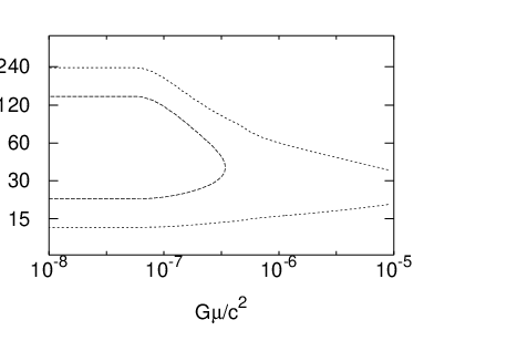

In Figure 17, we show the 68% and 95% confidence contours in string space using all surveys and the multifilter GO fields. We also show the analogous contours calculated using surveys and all GO fields. For surveys and multifilter data, our 95% confidence limits are , and . Using all of our data, our 95% confidence limits are , and . Our limits on are particularly sensitive on the prior we take in Eq. 22, but we have lowered the expected value of from 60 (the prior) to 52 (using GO-M) or 32 (using all data).
9 Discussion
Our string constraints could be lowered somewhat by new data that will soon be delivered by several different projects. The recently deployed HST Wide Field Camera 3 will provide 7 square arcminute exposures of high resolution data with similar limiting magnitudes to the Advanced Camera for Surveys (Kimble et al., 2006): this new GO data, combined with the growing ACS imaging archive should provide at least a factor of two increase in sky coverage. Looking ahead, the James Webb Space Telescope (JWST) is scheduled to launch in 2014, and will provide more images of similar depth and resolution to HST in the infrared (Gardner et al., 2006), albeit over smaller ( square arcmin) fields of view (and which may already have been observed in the optical with HST). These data would certainly enable the constraint projected in the “doubled dataset” curve in the right-hand panel of Figure 16.
Can we envision extending this study to much larger surveys? As we showed in Paper I, large ground-based projects like the Dark Energy Survey (The Dark Energy Survey Collaboration, 2005), the Panoramic Survey Telescope and Rapid Response System (Pan-STARRS) (Jedicke et al., 2007) and the Large Synoptic Survey Telescope (LSST)(Ivezic et al., 2008) would provide sufficient area and source counts for string searches, but lack the angular resolution to further constrain . Weak lensing surveys have been proposed for the Joint Dark Energy Mission (JDEM) that cover 10000 square degrees to an AB limiting magnitude of 26 (Aldering et al., 2004), although the exact details of the JDEM mission are still in flux (Gehrels & Albrecht, 2009).
Searching through more data will indeed lower our detection limits. If we were to double the number of HST fields we searched through, our 95% confidence limits would fall by a factor of 2–3 to and . The proposed JDEM survey would lower these confidence limits by a further factor of just 1.7 to and : a marginal improvement over the doubled HST limits, given the 3 orders of magnitude increase in survey area! At this point, resolution, and not lack of data would be the limiting factor. In fact, we argue that with this work we have within sight of the realm of diminishing returns, with only the next factor of two increase in survey scale gaining us a factor of two in parameter constraints.
The computational and human requirements for this work are modest and could be easily scaled up to analyse the forthcoming increased HST archive dataset. We did not use any special computational tools other than parallel batch processing, and all computation times quoted below are for modest desktop processors. We produced 6000 full HST-size simulated string images and 120000 10” wide string images (see Section 4) automatically in one month of processing time. The first round of automatic analysis (see Section 5.4) was performed on simulated data in one week and on all HST data in three days. The manual filtering described in Section 5.5 was performed on automatically-generated webpages for each field and required an average of twenty seconds per potential string for a total of ten hours of human work. In the future, the extraction of cosmic rays and other false sources would need to be automated for JDEM-scale datasets; the greater uniformity of such a survey’s images would make this process easier. The final automated phase described in Section 5.5 took essentially no computer time. The analysis of the remaining candidates (see Section 7.1) took several hours and would have to be automated for larger projects.
The technique for long string detection developed here will continue to be applicable to wider searches for lower tension, smaller image separation, and more sparsely distributed strings. Previous direct detection methods relied on finding single distinctive string lensing events (Sazhin et al., 2007) or searched for a large excess of similar pairs (Christiansen et al., 2008). The former method requires bright sources at large separation and thus does not make full use of survey depth or resolution. This prevents it from probing the smallest . In addition, it is difficult to characterise a single pair as being caused by a string lensing event. The latter method does not efficiently extract string lensing events from the background and is only effective if the field is crowded with strings. By searching for several pairs along straight lines, we probe to smaller separations (which imply smaller ), examine fainter sources (whose exponentially large number allow us to probe smaller ) and limit the possibility that a real string will be obscured by background pairs.
However, there are several straightforward improvements one could make to our string searching methods that could improve both the final limits and the searching efficiency in future projects. Firstly, our pair characterisation, based on magnitude, ellipticity and the alignment of a pair with the proposed string, does not use all the information available, and is unable to recognise a very incompletely copied pair. One could instead match the images of each pair pixel by pixel (Agol et al., 2006, as performed by), and allow incomplete copying to account for galaxy images “cut” by the string. We did not not implement this method on the grounds that our search focuses on barely resolved pairs for which there is little information, and because it would vastly increase computational time. One could imagine a hybrid survey whereby candidate image pairs were fed to an automated pixel-matching routine; this would both improve the purity of the candidate samples and also reduce the human inspection time of the search.
Using exclusively multifilter data would also make searching more efficient. None of our automatic string detection algorithms use color information because both COSMOS and half of the HAGGLeS GO fields are single filter. But we saw in Section 7 that checking for color consistency across pairs effectively eliminates potential string candidates. It may be impossible to guarantee multifilter data for large, diverse archival datasets like the GO fields, but the kind of homogeneous survey like JDEM would automatically provide color information which could be profitably exploited.
The main reason why our limits on string concentration and tension are much stricter than those of previous works is our use of a survey comprised of many scattered small fields. Because the probability of a string crossing a field scales as the linear size of the field and not its area, searching for cosmic strings in randomly scattered fields is more effective than searching many contiguous fields in a survey. This method also has the practical advantage that it does not require a dedicated survey and naturally thrives on archival data. Essentially any high resolution extragalactic images without overwhelmingly large objects in them can contribute to our limits on cosmic strings. However, the relatively small size of the ACS field means that at the low lensing cross-sections of interest we only expect to see a small number of lensed image pairs per field. This may be a problem for string searches based on the smaller WFC3 and JWST fields of view.
10 Conclusions
From an exhaustive search of some 4.5 square degrees of archival HST/ACS imaging data, we have derived significant direct detection limits on the tension and density of cosmic strings, employing a variety of techniques that could be applied to future searches. We draw the following conclusions:
- •
Using multi-filter data from the HAGGLeS, COSMOS, GEMS, AEGIS and GOODS surveys, we are able to constrain the dimensionless string tension to be below and the energy density in long strings to be below with 95% confidence.
- •
Extending the search to single filter GO imaging, we found 4 string candidates that we were unable to reject formally on the basis of the data in hand. Applying our experience with the multi-band data, we suggest that these detections are false positives: under this assumption we find stronger upper limits of and .
- •
Unlike previous optical imaging searches, we cover sufficient sky area to make these limits universal: if there were cosmic strings present in the redshift universe with tension and density greater than our limits, we would have detected them.
- •
Color information was found to be important in rejecting string candidates: high resolution imaging in multiple filters would be the most efficient way of ruling out the candidates presented here, and any future single-filter detections.
- •
Using the technology developed in this study, the upcoming factor of two increase in sky area imaged at comparably high resolution expected from the refurbished HST should enable these upper limits on string tension and density to be further reduced, by slightly more than a factor of two.
This work represents the the first direct detection limits on cosmic strings that are both competitive with and complimentary to other indirect methods. Our limit on the string tension is only a factor of 2–3 higher than the indirect upper limit of derived from the CMB power spectrum. We have shown that direct detection of strings by their gravitational lensing effect has the advantage of constraining both and , and does not require that strings emit gravitational radiation, as the pulsar timing constraints require. Perhaps most importantly, direct detection is the only method currently available that would provide the precise location of a cosmic string for future study. Prospects for using near future data to improve upon these limits are bright; however, we anticipate that this will bring us into the era where large increases in survey area would bring relatively small changes in the limits. The next significant advance in this field maybe the increase in angular resolution promised by future radio surveys.
Acknowledgments
We thank Joe Polchinski for inspiring this work with a Blackboard Lunch Talk at the Kavli Institute for Theoretical Physics (KITP), and for numerous useful suggestions. We are also very grateful for input to the early part of this project on the theoretical side from Alice Gasparini and Florian Dubath. We acknowledge Chris Fassnacht’s efforts in testing the HAGGLeS image processing pipeline and thank David Hogg for useful discussions about automated string detection. PJM received support from the TABASGO foundation in the form of a research fellowship. TT acknowledges support from the NSF through CAREER award NSF-0642621, and from the Sloan Foundation through a Sloan Research Fellowship. Support for this work was provided by NASA through grant number HST-AR-10676 (the HAGGLeS project) from the Space Telescope Science Institute, which is operated by AURA, Inc., under NASA contract NAS 5-26 555. This work was supported by the NSF under award AST05-07732 and in part by the U.S Department of Energy under contract number DE-AC02-76SF00515.
Appendix: The Probability of a 1 Radian String Crossing a Field
When calculating the probability of a rectangular, field lying on a projected radian string such that string crosses the field, we start by making useful approximations and other simplifications. We use the fact that our fields are much smaller than a radian so that the sky can be approximated as a rectangle with area steradians. We ignore the end effects and curvature of the string. As shown in Fig. 18, we imagine that the centre of our field is a distance from our string, and our field is oriented with the angle where implies that the long sides of our field (with length ) are perpendicular to the string. We need only consider the cases where and . The rest of parameter space is proportional by symmetry. The probability of a string crossing our field with toal overlap is then:
| (62) |

From Fig. 18, we can see that the vertical displacement between each of the three corners and the string is:
| (63) | |||||
| (64) | |||||
| (65) |
Where and .
A string can cross our field in three different ways: along the short axis (), along the long axis () or cutting a corner. If the string crosses our field along the short axis (entering and exiting via the two long sides), it’s crossing length is:
| (66) |
Using Eq. 62 we can convert this into the component of that represents the string crossing the field along the short axis, :
| (67) | |||||
| (68) | |||||
| (69) | |||||
If a string crosses along the long side of the field:
| (70) |
And:
| (71) |
When the string “cuts the corner”, entering and exiting via adjacent sides, is:
| (72) | |||||
Again using Eq. 62 we can find the component of that comes from the string crossing the field via adjacent sides, :
| (73) | |||||
| (74) |
and mark the points when a second corner rotates across the string so that reverts to either or . We can derive them from Eq. 64 and Eq. 65 and obtain:
| (77) | |||||
| (78) | |||||
| (79) | |||||
| (80) |
Finally, we add , and to obtain:
| (81) | |||||
References
- Accetta & Krauss (1989) Accetta, F. S., & Krauss, L. M. 1989, Physics Letters B, 233, 93
- Agol et al. (2006) Agol, E., Hogan, C. J., & Plotkin, R. M. 2006, Phys.Rev.D, 73, 087302
- Aldering et al. (2004) Aldering, G., et al. 2004, arXiv:astro-ph/0405232
- Allen & Shellard (1990) Allen, B., & Shellard, E. P. S. 1990, Phys. Rev. Lett., 64, 119
- Ballester (1996) Ballester, P. 1996, Vistas in Astronomy, 40, 479
- Benitez et al. (2003) Benitez, N., et al. 2003, ArXiv Astrophysics e-prints
- Bertin & Arnouts (1996) Bertin, E., & Arnouts, S. 1996, A&AS, 117, 393
- Bouchet (2007) Bouchet, F. R. 2007, Modern Physics Letters A, 22, 1857
- Caldwell & Allen (1992) Caldwell, R. R., & Allen, B. 1992, Phys.Rev.D, 45, 3447
- Christiansen et al. (2008) Christiansen, J. L., Albin, E., James, K. A., Goldman, J., Maruyama, D., & Smoot, G. F. 2008, ArXiv e-prints
- Coleman et al. (1980) Coleman, G. D., Wu, C.-C., & Weedman, D. W. 1980, ApJS, 43, 393
- Damour & Vilenkin (2005) Damour, T., & Vilenkin, A. 2005, Phys.Rev.D, 71, 063510
- Davis et al. (2007) Davis, M., et al. 2007, ApJ, 660, L1
- de Laix (1997) de Laix, A. A. 1997, Phys.Rev.D, 56, 6193
- Fowler et al. (2007) Fowler, J. W., et al. 2007, Appl.Optics, 46, 3444
- Gardner et al. (2006) Gardner, J. P., et al. 2006, Space Science Reviews, 123, 485
- Gasparini et al. (2008) Gasparini, M. A., Marshall, P., Treu, T., Morganson, E., & Dubath, F. 2008, MNRAS, 385, 1959
- Gehrels & Albrecht (2009) Gehrels, N., & Albrecht, A. 2009, APS Meeting Abstracts, F1001+
- Giavalisco et al. (2004) Giavalisco, M., et al. 2004, ApJ, 600, L93
- Hindmarsh & Kibble (1995) Hindmarsh, M. B., & Kibble, T. W. B. 1995, Reports on Progress in Physics, 58, 477
- Huterer & Vachaspati (2003) Huterer, D., & Vachaspati, T. 2003, Phys.Rev.D, 68, 041301
- Ivezic et al. (2008) Ivezic, Z., Tyson, J. A., Allsman, R., Andrew, J., Angel, R., & for the LSST Collaboration. 2008, ArXiv e-prints, 805
- Jedicke et al. (2007) Jedicke, R., Magnier, E. A., Kaiser, N., & Chambers, K. C. 2007, in IAU Symposium, Vol. 236, IAU Symposium, ed. G. B. Valsecchi & D. Vokrouhlický, 341–352
- Jeong & Smoot (2007) Jeong, E., & Smoot, G. F. 2007, ApJ, 661, L1
- Kaspi et al. (1994) Kaspi, V. M., Taylor, J. H., & Ryba, M. F. 1994, ApJ, 428, 713
- Kibble (1976) Kibble, T. W. B. 1976, J. Phys. A: Math. Gen. 9, 1387
- Kibble (2004) —. 2004, ArXiv Astrophysics e-prints
- Kimble et al. (2006) Kimble, R. A., MacKenty, J. W., & O’Connell, R. W. 2006, in Presented at the Society of Photo-Optical Instrumentation Engineers (SPIE) Conference, Vol. 6265, Space Telescopes and Instrumentation I: Optical, Infrared, and Millimeter. Edited by Mather, John C.; MacEwen, Howard A.; de Graauw, Mattheus W. M.. Proceedings of the SPIE, Volume 6265, pp. 62650I (2006).
- Leauthaud et al. (2007) Leauthaud, A., et al. 2007, ApJS, 172, 219
- Lo & Wright (2005) Lo, A. S., & Wright, E. L. 2005, arXiv:astro-ph/0503120
- Mack et al. (2007) Mack, K. J., Wesley, D. H., & King, L. J. 2007, Phys.Rev.D, 76, 123515
- Morganson & Blandford (2008) Morganson, E., & Blandford, R. 2008, ArXiv e-prints
- Muchovej et al. (2007) Muchovej, S., et al. 2007, in Bulletin of the American Astronomical Society, Vol. 38, Bulletin of the American Astronomical Society, 996–+
- Oguri & Takahashi (2005) Oguri, M., & Takahashi, K. 2005, Phys.Rev.D, 72, 085013
- Pogosian et al. (2006) Pogosian, L., Tye, S.-H. H., Wasserman, I., & Wyman, M. 2006, Phys.Rev.D, 73, 089904
- Pogosian et al. (2004) Pogosian, L., Wyman, M., & Wasserman, I. 2004, Journal of Cosmology and Astro-Particle Physics, 9, 8
- Polchinski (2004a) Polchinski, J. 2004a, 743, 331
- Polchinski (2004b) Polchinski, J. 2004b, in Lectures presented at the 2004 Cargese Summer School
- Polchinski (2007) Polchinski, J. 2007, in Proceedings of the Eleventh Marcel Grossmann Meeting on General Relativity, ed. R. J. H. Kleinert & R. Ruffini (World Scientific: Singapore)
- Rix et al. (2004) Rix, H.-W., et al. 2004, ApJS, 152, 163
- Rocha (2008) Rocha, J. V. 2008, ArXiv e-prints
- Sazhin & Khlopov (1989) Sazhin, M. V., & Khlopov, M. Y. 1989, Soviet Astronomy, 33, 98
- Sazhin et al. (2007) Sazhin, M. V., Khovanskaya, O. S., Capaccioli, M., Longo, G., Paolillo, M., Covone, G., Grogin, N. A., & Schreier, E. J. 2007, MNRAS, 376, 1731
- Sazhina et al. (2008) Sazhina, O. S., Sazhin, M. V., & Sementsov, V. N. 2008, Soviet Journal of Experimental and Theoretical Physics, 106, 878
- Scoville et al. (2007) Scoville, N., et al. 2007, ApJS, 172, 38
- Stewart & Brandenberger (2009) Stewart, A., & Brandenberger, R. 2009, Journal of Cosmology and Astro-Particle Physics, 2, 9
- The Dark Energy Survey Collaboration (2005) The Dark Energy Survey Collaboration. 2005, ArXiv Astrophysics e-prints
- Timothy et al. (2009) Timothy, F., James, K. A., & Christiansen, J. 2009, in Bulletin of the American Astronomical Society, Vol. 41, Bulletin of the American Astronomical Society, 445–+
- Vilenkin (1984) Vilenkin, A. 1984, ApJ, 282, L51
- Vilenkin & Shellard (1994) Vilenkin, A., & Shellard, E. P. S. 1994, Cosmic strings and other topological defects, ed. A. Vilenkin & E. P. S. Shellard
- Zwart et al. (2008) Zwart, J. T. L., et al. 2008, MNRAS, 391, 1545