跳到论文正文
W Papers独立论文阅读器 arXiv:0908.0582 论文正文 计算阅读时间 · 0%
引用这篇论文根据当前论文元数据生成,正式投稿前建议核对。


License: arXiv.org perpetual non-exclusive license
arXiv:0908.0582v2 [math.NT] 24 Feb 2010

On the recurrence of coefficients in the Lück-Fuglede-Kadison determinant

Oliver T. Dasbach    Matilde N. Lalin
Abstract

In this note, we survey results concerning variations of the Lück-Fuglede-Kadison determinant with respect to the base group. Further, we discuss recurrences of coefficients in the determinant for certain distinguished base groups. The note is based on a talk that the second author gave at the “Segundas Jornadas de Teoría de Números”, Madrid, 2007.

The object that we consider in this note is given by the following

Definition 1.

[DL09] Let Γ\Gamma be a group finitely generated by x1,…,xlx_{1},\dots,x_{l}. Let P=∑g∈Γcg​g∈ℂ​ΓP=\sum_{g\in\Gamma}c_{g}g\in\mathbb{C}\Gamma such that cg=cg−1¯c_{g}=\overline{c_{g^{-1}}}. Let λ\lambda be a small complex number. More precisely, |λ|<1l1​(P)|\lambda|<\frac{1}{l_{1}(P)}, the reciprocal of the sum of the absolute values of the coefficients of PP. The Mahler measure (or Lück-Fuglede-Kadison determinant [Lue02]) of 1−λ​P1-\lambda P is given by

mΓ(P,λ)=−∑n=1∞an​λnn,m_{\Gamma}(P,\lambda)=-\sum_{n=1}^{\infty}\frac{a_{n}\lambda^{n}}{n},

where an=[Pn]0a_{n}=[P^{n}]_{0} is the constant coefficient of the nn-th power of PP; in other words, ana_{n} is the trace of the element Pn∈ℂ​ΓP^{n}\in\mathbb{C}\Gamma.

We will often consider the generating function for the ana_{n}’s

uΓ​(P,λ)=∑n=0∞an​λn.u_{\Gamma}(P,\lambda)=\sum_{n=0}^{\infty}a_{n}\lambda^{n}.

Thus,

uΓ​(P,λ)=a0−λ​dd​λ​mΓ​(P,λ).u_{\Gamma}(P,\lambda)=a_{0}-\lambda\frac{\mbox{d}}{\mbox{d}\lambda}m_{\Gamma}(P,\lambda).

1 Summary of previous results

We have studied in [DL09] some properties of mΓ​(P,λ)m_{\Gamma}(P,\lambda) where we emphasize the variation of Γ\Gamma. For particular cases of Γ\Gamma one can find formulas for the Mahler measure over Γ\Gamma. In the following formulas, |λ|<1l1​(P)|\lambda|<\frac{1}{l_{1}(P)}.

  • •

    If Γ=ℤh\Gamma=\mathbb{Z}^{h},

    (1) Re(mΓ​(P,λ))=m⁡(1−λ​P),\mathop{\mathrm{Re}}(m_{\Gamma}(P,\lambda))=m(1-\lambda P),

    where the term on the right hand-side indicates the Mahler measure in the classical sense,

    m⁡(1−λ​P)=1(2​π​i)h​∫𝕋hlog⁡|1−λ​P​(x1,…,xh)|​d​x1x1​…​d​xhxh.m(1-\lambda P)=\frac{1}{(2\pi\mathrm{i})^{h}}\int_{\mathbb{T}^{h}}\log|1-\lambda P(x_{1},\dots,x_{h})|\frac{\;\mathrm{d}x_{1}}{x_{1}}\dots\frac{\;\mathrm{d}x_{h}}{x_{h}}.

    Here 𝕋h={|x1|=⋯=|xh|=1}\mathbb{T}^{h}=\{|x_{1}|=\dots=|x_{h}|=1\} is the hh-th unit torus.

  • •

    If Γ\Gamma is finite,

    (2) mΓ​(P,λ)=1|Γ|​log​det(1−λ​A),m_{\Gamma}(P,\lambda)=\frac{1}{|\Gamma|}\log\det(1-\lambda A),

    where AA is the adjacency matrix of a weighted Cayley graph of Γ\Gamma generated by the monomials of PP (see [DL09]) and we are considering the main branch of the logarithm. This formula provides a meromorphic continuation of the Mahler measure mΓ​(P,λ)m_{\Gamma}(P,\lambda) to the complex plane minus Spec​(A)\mbox{Spec}(A).

  • •

    If Γ=ℤ/m1​ℤ×⋯×ℤ/mh​ℤ\Gamma=\mathbb{Z}/m_{1}\mathbb{Z}\times\dots\times\mathbb{Z}/m_{h}\mathbb{Z}, then

    (3) mΓ​(P,λ)=1|Γ|​log⁡(∏j1,…,jh(1−λ​P​(ξm1j1,…,ξmhjh))),m_{\Gamma}(P,\lambda)=\frac{1}{|\Gamma|}\log\left(\prod_{j_{1},\dots,j_{h}}(1-\lambda P(\xi_{m_{1}}^{j_{1}},\dots,\xi_{m_{h}}^{j_{h}}))\right),

    where ξm\xi_{m} denotes an mm-th primitive root of the unity, and again, we are considering the main branch of the logarithm.

Of further interest are approximation results for the Mahler measure over infinite groups. In [DL09] it is shown that

  • •
    (4) limmi→∞mℤ/m1​ℤ×⋯×ℤ/mh​ℤ​(P,λ)=mℤh​(P,λ)\lim_{m_{i}\rightarrow\infty}m_{\mathbb{Z}/m_{1}\mathbb{Z}\times\dots\times\mathbb{Z}/m_{h}\mathbb{Z}}(P,\lambda)=m_{\mathbb{Z}^{h}}(P,\lambda)
  • •
    (5) limm→∞mDm​(P,λ)=mD∞​(P,λ)\lim_{m\rightarrow\infty}m_{D_{m}}(P,\lambda)=m_{D_{\infty}}(P,\lambda)

    Here DmD_{m} is the dihedral group Dm=⟨ρ,σ|ρm,σ2,σρσρ⟩D_{m}=\langle\rho,\sigma|\rho^{m},\sigma^{2},\sigma\rho\sigma\rho\rangle and D∞=⟨ρ,σ|σ2,σρσρ⟩D_{\infty}=\langle\rho,\sigma|\sigma^{2},\sigma\rho\sigma\rho\rangle.

2 Recurrence relations

Following the ideas in [RV99], notice that if Γ=ℤl\Gamma=\mathbb{Z}^{l}, then

u⁡(λ)=1(2​π​i)l​∫𝕋lω⁡(λ)whereω⁡(λ)=11−λ​P​(x1,…,xl)​d​x1x1​…​d​xlxl.u(\lambda)=\frac{1}{(2\pi\mathrm{i})^{l}}\int_{\mathbb{T}^{l}}\omega(\lambda)\hskip 20.00003pt\mathrm{where}\hskip 10.00002pt\omega(\lambda)=\frac{1}{1-\lambda P(x_{1},\dots,x_{l})}\frac{\;\mathrm{d}x_{1}}{x_{1}}\dots\frac{\;\mathrm{d}x_{l}}{x_{l}}.

For each value of λ\lambda, u⁡(λ)u(\lambda) is a period of ω⁡(λ)\omega(\lambda) in ℙl​(ℂ)\mathbb{P}^{l}(\mathbb{C}). The integral depends on the homology class of 𝕋l\mathbb{T}^{l} in Hl​(ℙl​(ℂ)∖V,ℤ)H_{l}(\mathbb{P}^{l}(\mathbb{C})\setminus V,\mathbb{Z}), where VV is the zero locus of the denominator in the rational function (which is generically non-singular as λ\lambda varies). See Griffiths [Gri69].

Now if we take successive derivatives of ω⁡(λ)\omega(\lambda), we obtain several differential forms that belong to a subspace of the de Rham cohomology Hl​(V)H^{l}(V) which has finite dimension. Griffiths proves that u⁡(λ)u(\lambda) satisfies a Picard-Fuchs differential equation

pk​(λ)​u(k)+pk−1​(λ)​u(k−1)+⋯+p0​(λ)​u=0,p_{k}(\lambda)u^{(k)}+p_{k-1}(\lambda)u^{(k-1)}+\dots+p_{0}(\lambda)u=0,

where the pip_{i} are polynomials in λ\lambda, see [Gri69] for details.

From such a differential equation it is easy to deduce a linear recurrence with polynomial coefficients for the coefficients an=[Pn]0a_{n}=[P^{n}]_{0} of u⁡(λ)u(\lambda).

One can extend this more generally:

Theorem 2.

If Γ\Gamma is a finitely generated abelian group then the coefficients an=[Pn]0a_{n}=[P^{n}]_{0} satisfy a linear recurrence relation with polynomial coefficients.

PROOF.  Let Γ=ℤl×ℤ/m1​ℤ×⋯×ℤ/mh​ℤ\Gamma=\mathbb{Z}^{l}\times\mathbb{Z}/m_{1}\mathbb{Z}\times\dots\times\mathbb{Z}/m_{h}\mathbb{Z}. Combining Equation (3) and the techniques that are used in the proof of Equation (4) (see [DL09]), we obtain that

mΓ​(P,λ)=1m1​…​mh​∑j1,…,jhm⁡(P⁡(x1,…,xl,ξm1j1,…,ξmhjh),λ),m_{\Gamma}(P,\lambda)=\frac{1}{m_{1}\dots m_{h}}\sum_{j_{1},\dots,j_{h}}m(P(x_{1},\dots,x_{l},\xi_{m_{1}}^{j_{1}},\dots,\xi_{m_{h}}^{j_{h}}),\lambda),

where ξk\xi_{k} is a primitive root of unity, and the sum on the right involves Mahler measures in the classical (abelian) sense.

Then the result follows easily since it is known for Mahler measures.

∎

For finite groups, we have the following

Theorem 3.

If Γ\Gamma is a finite group, then the coefficients an=[Pn]0a_{n}=[P^{n}]_{0} satisfy a recurrence relation (with constant coefficients) of length at most |Γ||\Gamma|.

PROOF.  In the proof of Equation (3) (Theorem 6 in [DL09]) we write

an=1|Γ|​tr​(An).a_{n}=\frac{1}{|\Gamma|}\mathrm{tr}(A^{n}).

Any polynomial that annihilates AA yields a recurrence relation with constant coefficients for ana_{n}. In particular, the characteristic polynomial yields a bound for the length of the recurrence.

∎

More is known in the case where Γ\Gamma is free [BG07]: the function u⁡(λ)u(\lambda) turns out to be algebraic. A proof for this uses algebraic functions in non-commuting variables and a theorem of Haiman [Hai93]; see [BG07] for details.

A natural question is the following: can we say anything for “intermediate” groups?

3 Some examples

Of particular interest is the case when Pl=x1+x1−1+⋯+xl+xl−1P_{l}=x_{1}+x_{1}^{-1}+\dots+x_{l}+x_{l}^{-1} where x1,…,xlx_{1},\dots,x_{l} are the generators in a given group presentation of the group Γ\Gamma.

It is easy to see that [Pln]0[P_{l}^{n}]_{0} has the following interpretation

Lemma 4.

The number of closed circuits based at the origin in the Cayley graph of Γ\Gamma - with respect to the generators x1,…,xlx_{1},\dots,x_{l} in the presentation - is given by [Pln]0[P_{l}^{n}]_{0}.

3.1 Abelian groups

Consider the example of P2=x+x−1+y+y−1P_{2}=x+x^{-1}+y+y^{-1} with group Γ=ℤ2\Gamma=\mathbb{Z}^{2}. Then one obtains (see for example [Dom60, RV99])

u⁡(λ)=∑n=0∞(2​nn)2​λ2​n.u(\lambda)=\sum_{n=0}^{\infty}\binom{2n}{n}^{2}\lambda^{2n}.

Since we only have terms with even degree, we reparametrize,

v⁡(μ)=∑n=0∞(2​nn)2​μn.v(\mu)=\sum_{n=0}^{\infty}\binom{2n}{n}^{2}\mu^{n}.

Then the differential equation is given by [RV99]

μ⁡(16​μ−1)​v′′+(32​μ−1)​v′+4​v=0.\mu(16\mu-1)v^{\prime\prime}+(32\mu-1)v^{\prime}+4v=0.

From such a differential equation it is possible to deduce a recurrence of the coefficients, in this case, a0=1,a2=4a_{0}=1,a_{2}=4, and

n2​a2​n−4​(2​n−1)2​a2​n−2=0.n^{2}a_{2n}-4(2n-1)^{2}a_{2n-2}=0.

Of course this equation can be easily deduced from the formula for ana_{n}.

If one considers one more variable, P3=x+x−1+y+y−1+z+z−1P_{3}=x+x^{-1}+y+y^{-1}+z+z^{-1}. Then one obtains

u⁡(λ)=∑n=0∞(2​nn)​∑k=0n(nk)2​(2​kk)​λ2​n,u(\lambda)=\sum_{n=0}^{\infty}\binom{2n}{n}\sum_{k=0}^{n}\binom{n}{k}^{2}\binom{2k}{k}\lambda^{2n},

and a0=1,a2=6,a4=90a_{0}=1,a_{2}=6,a_{4}=90,

(6) n3​a2​n−2​(2​n−1)​(10​n2−10​n+3)​a2​n−2+36​(2​n−1)​(n−1)​(2​n−3)​a2​n−4=0.n^{3}a_{2n}-2(2n-1)(10n^{2}-10n+3)a_{2n-2}+36(2n-1)(n-1)(2n-3)a_{2n-4}=0.

As observed in [DL09], for ll variables, we obtain

(7) a2​n(Pl)=∑j1+⋯+jl=n(2​n)!(j1!)2​…​(jl!)2.a_{2n}^{(P_{l})}=\sum_{j_{1}+\dots+j_{l}=n}\frac{(2n)!}{(j_{1}!)^{2}\dots(j_{l}!)^{2}}.

By Lemma 4 these coefficients can be interpreted as the number of circuits of length 2​n2n (that start and end at the origin) in the ll-dimensional cubic lattice.

Another polynomial that is interesting to study is

Ql=(1+x1+⋯+xl−1)​(1+x1−1+⋯+xl−1−1).Q_{l}=(1+x_{1}+\dots+x_{l-1})(1+x_{1}^{-1}+\dots+x_{l-1}^{-1}).

One has [DL09] that

(8) an(Ql)=∑j1+⋯+jl=n(n!j1!​…​jl!)2.a_{n}^{(Q_{l})}=\sum_{j_{1}+\dots+j_{l}=n}\left(\frac{n!}{j_{1}!\dots j_{l}!}\right)^{2}.

We see that the terms in equation (7) correspond to the one in (8) multiplied by (2​nn)\binom{2n}{n}, and that allows an easy translation for the recurrences. If

∑k=0l−1pk​(n)​a2​n−2​k(Pl)=0,\sum_{k=0}^{l-1}p_{k}(n)a_{2n-2k}^{(P_{l})}=0,

then

(9) ∑k=0l−1(n!)2​(2​n−2​k)!((n−k)!)2​(2​n−2​l+2)!​pk​(n)​an−k(Ql)=0.\displaystyle\sum_{k=0}^{l-1}\frac{(n!)^{2}(2n-2k)!}{((n-k)!)^{2}(2n-2l+2)!}p_{k}(n)a_{n-k}^{(Q_{l})}=0.

As an example, for l=3l=3 we have

Q3=(1+x+y)​(1+x−1+y−1)=3+x+x−1+y+y−1+x​y−1+x−1​y.Q_{3}=(1+x+y)(1+x^{-1}+y^{-1})=3+x+x^{-1}+y+y^{-1}+xy^{-1}+x^{-1}y.

One obtains a0=1,a1=15a_{0}=1,a_{1}=15,

n2​an−(10​n2−10​n+3)​an−1+9​(n−1)2​an−2=0,n^{2}a_{n}-(10n^{2}-10n+3)a_{n-1}+9(n-1)^{2}a_{n-2}=0,

from Equations (6) and (9).

Furthermore, from the above discussion a closed form is given by (see also [CRRS02, Dom60])

an=∑k=0n(nk)2​(2​kk),a_{n}=\sum_{k=0}^{n}\binom{n}{k}^{2}\binom{2k}{k},

and with the notations of this section:

[P32​n]0=(2​nn)​an=(2​nn)​[Q3n]0.[P_{3}^{2n}]_{0}=\binom{2n}{n}a_{n}=\binom{2n}{n}[Q_{3}^{n}]_{0}.

Also note that bn:=[P3n]0=[(Q3−3)n]0b_{n}:=[P_{3}^{n}]_{0}=[(Q_{3}-3)^{n}]_{0} is related to ana_{n} by

bn=∑j=0n(nj)​(−3)n−j​aj.b_{n}=\sum_{j=0}^{n}\binom{n}{j}(-3)^{n-j}a_{j}.

One can show that bnb_{n} satisfies the recursion: b0=1,b1=0,b2=6b_{0}=1,b_{1}=0,b_{2}=6,

n2​bn−n⁡(n−1)​bn−1−24​(n−1)2​bn−2−36​(n−2)​(n−1)​bn−3=0.n^{2}b_{n}-n(n-1)b_{n-1}-24(n-1)^{2}b_{n-2}-36(n-2)(n-1)b_{n-3}=0.

The numbers ana_{n} and bnb_{n} have an interesting interpretation. Since

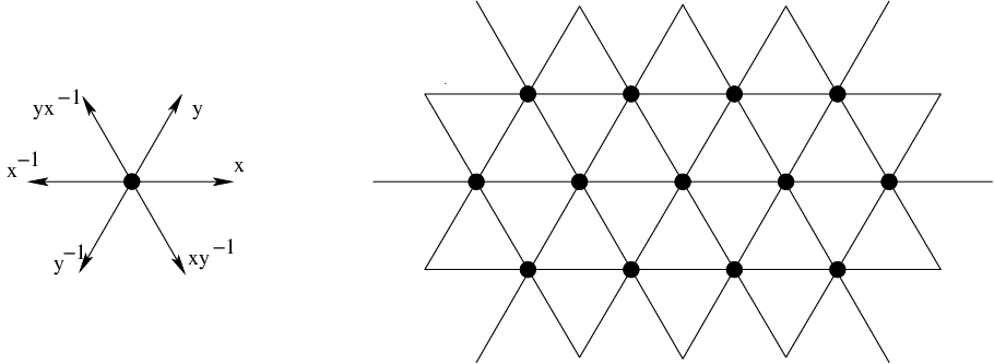
Q3−3=x+x−1+y+y−1+x​y−1+x−1​yQ_{3}-3=x+x^{-1}+y+y^{-1}+xy^{-1}+x^{-1}y

the constant coefficient bnb_{n} in (Q3−3)n(Q_{3}-3)^{n} counts the number of closed circuits of length nn, based at a fixed point, in the triangular lattice that is depicted in Figure 1.
Refer to caption
Figure 1: The triangular lattice: An edge in the lattice corresponds to a multiplication in ℤ2\mathbb{Z}^{2}.

A look at the honeycomb lattice in Figure 2 reveals that at any point there are nine different paths of length two originating from that point. Three are closed paths the other six can be labeled by x,x−1,y,y−1,x​y−1x,x^{-1},y,y^{-1},xy^{-1} and x−1​yx^{-1}y as in the triangular lattice (Figure 1). It follows that ana_{n} is the number of closed circuits in the honeycomb lattice of length 2​n2n that are based at a fixed point.

Refer to caption
Figure 2: The honeycomb lattice.

Our motivation for studying the above examples comes from the fact that

m⁡(1+x+y)=12​m​((1+x+y)​(1+x−1+y−1))m(1+x+y)=\frac{1}{2}m((1+x+y)(1+x^{-1}+y^{-1}))

and

m⁡(1+x+y)=3​34​π​L​(χ−3,2)=D⁡(e2​π​i3)π=Vol⁡(Fig​ 8)2​πm(1+x+y)=\frac{3\sqrt{3}}{4\pi}\mathrm{L}(\chi_{-3},2)=\frac{D\left(\mathrm{e}^{\frac{2\pi\mathrm{i}}{3}}\right)}{\pi}=\frac{\mathrm{Vol}(\mathrm{Fig}\,8)}{2\pi}

Here, Vol⁡(Fig​ 8)\mathrm{Vol}(\mathrm{Fig}\,8) is the hyperbolic volume of the Figure-8 knot complement. The first equality was computed by Smyth [Smy81] and the last one was observed by Boyd [Boy02].

It follows that for λ\lambda sufficiently small we have:

Vol⁡(Fig​ 8)π\displaystyle\frac{\mathrm{Vol}(\mathrm{Fig}\,8)}{\pi} =\displaystyle= 2​m​(1+x+y)=m⁡(Q3)=m⁡(1λ​(1−(1−λ​Q3)))\displaystyle 2m(1+x+y)=m(Q_{3})=m\left(\frac{1}{\lambda}(1-(1-\lambda Q_{3}))\right)
=\displaystyle= −log⁡λ+m⁡(1−(1−λ​Q3))\displaystyle-\log\lambda+m(1-(1-\lambda Q_{3}))
=\displaystyle= −log⁡λ−∑n=1∞cnn\displaystyle-\log\lambda-\sum_{n=1}^{\infty}\frac{c_{n}}{n}
=\displaystyle= −log⁡λ−∑n=1∞1n​∑k=0n(nk)​(−λ)k​ak\displaystyle-\log\lambda-\sum_{n=1}^{\infty}\frac{1}{n}\sum_{k=0}^{n}\binom{n}{k}(-\lambda)^{k}a_{k}
=\displaystyle= −log⁡λ−∑n=1∞1n​∑k=0n∑j=0k(nk)​(kj)2​(2​jj)​(−λ)k\displaystyle-\log\lambda-\sum_{n=1}^{\infty}\frac{1}{n}\sum_{k=0}^{n}\sum_{j=0}^{k}\binom{n}{k}{\binom{k}{j}}^{2}\binom{2j}{j}(-\lambda)^{k}

where cn:=[(1−λ​Q3)n]0c_{n}:=[(1-\lambda Q_{3})^{n}]_{0} and an=[Q3n]0a_{n}=[Q_{3}^{n}]_{0}.

This type of expression for the volume of the Figure-8 knot should be compared to Lück’s formula [Lue02, DL09] (Theorem 3). In that formula, the volume of a knot complement is expressed in terms of a similar formula, but the Mahler measure is computed over an element in the group ring of the fundamental group of the knot which is non-abelian. The coefficients in Lück’s formula are notably hard to compute in practice.

3.2 Predicting a recurrence relation from another recurrence relation

Recall that we saw that the circuits in the triangular lattice and the even ones in the honeycomb lattice are related by

bn=∑j=0n(nj)​(−3)n−j​aj.b_{n}=\sum_{j=0}^{n}\binom{n}{j}(-3)^{n-j}a_{j}.

More generally, in the previous example, we have that

cn=∑j=0n(nj)​(−λ)j​aj.c_{n}=\sum_{j=0}^{n}\binom{n}{j}(-\lambda)^{j}a_{j}.

Given a recurrence relation for the aja_{j} we would like to obtain a recurrence relation for the cjc_{j}. The first observation is that we can assume that −λ=1-\lambda=1, since it is easy to find a recurrence relation for (−λ)j​aj(-\lambda)^{j}a_{j} from the one for aja_{j}. In other words, we can assume

cn=∑j=0n(nj)​aj.c_{n}=\sum_{j=0}^{n}\binom{n}{j}a_{j}.

Consider one more time the generating function

u⁡(t)=∑n=0∞an​tn.u(t)=\sum_{n=0}^{\infty}a_{n}t^{n}.

For the cnc_{n} we have

v⁡(t)=∑n=0∞cn​tn=∑n=0∞∑j=0n(nj)​aj​tn.v(t)=\sum_{n=0}^{\infty}c_{n}t^{n}=\sum_{n=0}^{\infty}\sum_{j=0}^{n}\binom{n}{j}a_{j}t^{n}.

If |t||t| is small enough, we can invert the order in the sum,

v⁡(t)=∑j=0∞aj​∑n=0∞(nj)​tn.v(t)=\sum_{j=0}^{\infty}a_{j}\sum_{n=0}^{\infty}\binom{n}{j}t^{n}.

Now observe that

∑n=0∞(nj)​tn\displaystyle\sum_{n=0}^{\infty}\binom{n}{j}t^{n} =\displaystyle= tjj!∑n=0∞n⋯(n−j+1)tn−j=tjj!(11−t)(j)\displaystyle\frac{t^{j}}{j!}\sum_{n=0}^{\infty}n\cdots(n-j+1)t^{n-j}=\frac{t^{j}}{j!}\left(\frac{1}{1-t}\right)^{(j)}
=\displaystyle= tjj!​j!(1−t)j+1=tj(1−t)j+1.\displaystyle\frac{t^{j}}{j!}\frac{j!}{(1-t)^{j+1}}=\frac{t^{j}}{(1-t)^{j+1}}.

Putting everything together,

v⁡(t)=11−t​∑j=0∞aj​(t1−t)j.v(t)=\frac{1}{1-t}\sum_{j=0}^{\infty}a_{j}\left(\frac{t}{1-t}\right)^{j}.

Now, a recurrence relation for ana_{n} is equivalent to a differential equation for u⁡(t)u(t), which translates into a differential equation for v⁡(t)v(t) and from there one obtains a recurrence for cnc_{n}.

As an example let us compute the recurrence in the case of cnc_{n} with λ=16\lambda=\frac{1}{6}.

First, we set bn=an(−6)nb_{n}=\frac{a_{n}}{(-6)^{n}}. We have

n2​an−(10​n2−10​n+3)​an−1+9​(n−1)2​an−2=0.n^{2}a_{n}-(10n^{2}-10n+3)a_{n-1}+9(n-1)^{2}a_{n-2}=0.

Therefore,

(10) 12​n2​bn+2​(10​n2−10​n+3)​bn−1+3​(n−1)2​bn−2=0,12n^{2}b_{n}+2(10n^{2}-10n+3)b_{n-1}+3(n-1)^{2}b_{n-2}=0,

and

cn=∑j=0n(nj)​bj.c_{n}=\sum_{j=0}^{n}\binom{n}{j}b_{j}.

Let

u⁡(t)=∑n=0∞bn​tn,v⁡(t)=∑n=0∞cn​tn=11−t​∑n=0∞bn​(t1−t)n.u(t)=\sum_{n=0}^{\infty}b_{n}t^{n},\hskip 20.00003ptv(t)=\sum_{n=0}^{\infty}c_{n}t^{n}=\frac{1}{1-t}\sum_{n=0}^{\infty}b_{n}\left(\frac{t}{1-t}\right)^{n}.

Set s=t1−ts=\frac{t}{1-t}, then

(1−t)​v​(t)=u⁡(s).(1-t)v(t)=u(s).

Notice that recurrence (10) translates into the differential equation

12​t​(t​u′′+u′)+2​t​(10​t2​u′′+20​t​u′+u)+3​t2​(t2​u′′+3​t​u′+u)=0.12t(tu^{\prime\prime}+u^{\prime})+2t(10t^{2}u^{\prime\prime}+20tu^{\prime}+u)+3t^{2}(t^{2}u^{\prime\prime}+3tu^{\prime}+u)=0.

Hence,

t2​(t+6)​(3​t+2)​u′′+t⁡(9​t2+40​t+12)​u′+t⁡(3​t+2)​u=0.t^{2}(t+6)(3t+2)u^{\prime\prime}+t(9t^{2}+40t+12)u^{\prime}+t(3t+2)u=0.

We have

u′​(s)=(1−t)2​((1−t)​v′​(t)−v⁡(t)).u^{\prime}(s)=(1-t)^{2}((1-t)v^{\prime}(t)-v(t)).
u′′​(s)=(1−t)3​((1−t)2​v′′​(t)−4​(1−t)​v′​(t)+2​v​(t)).u^{\prime\prime}(s)=(1-t)^{3}((1-t)^{2}v^{\prime\prime}(t)-4(1-t)v^{\prime}(t)+2v(t)).

Replacing in

s2​(s+6)​(3​s+2)​u′′+s⁡(9​s2+40​s+12)​u′+s⁡(3​s+2)​u=0,s^{2}(s+6)(3s+2)u^{\prime\prime}+s(9s^{2}+40s+12)u^{\prime}+s(3s+2)u=0,

we obtain

t2​(t+2)​(5​t−6)​((1−t)2​v′′​(t)−4​(1−t)​v′​(t)+2​v​(t))t^{2}(t+2)(5t-6)((1-t)^{2}v^{\prime\prime}(t)-4(1-t)v^{\prime}(t)+2v(t))
+t⁡(19​t2−16​t−12)​((1−t)​v′​(t)−v⁡(t))+t⁡(t+2)​v​(t)=0.+t(19t^{2}-16t-12)((1-t)v^{\prime}(t)-v(t))+t(t+2)v(t)=0.

Thus

(5​t4−t3−16​t2+12​t)​v′′​(t)+(20​t3−3​t2−32​t+12)​v′​(t)(5t^{4}-t^{3}-16t^{2}+12t)v^{\prime\prime}(t)+(20t^{3}-3t^{2}-32t+12)v^{\prime}(t)
+(10​t2−t−10)​v​(t)=0.+(10t^{2}-t-10)v(t)=0.

Finally, the differential equation translates into the recurrence

12​n2​cn−2​(8​n2−8​n+5)​cn−1−(n−1)2​cn−2+5​(n−1)​(n−2)​cn−3=0,12n^{2}c_{n}-2(8n^{2}-8n+5)c_{n-1}-(n-1)^{2}c_{n-2}+5(n-1)(n-2)c_{n-3}=0,

with initial terms c0=1,c1=12,c2=512c_{0}=1,c_{1}=\frac{1}{2},c_{2}=\frac{5}{12}.

3.3 Free groups

If we reconsider the cases of Pl=x1+x1−1+⋯+xl+xl−1P_{l}=x_{1}+x_{1}^{-1}+\dots+x_{l}+x_{l}^{-1} and Ql=(1+x1+⋯+xl−1)​(1+x1−1+⋯+xl−1−1)Q_{l}=(1+x_{1}+\dots+x_{l-1})(1+x_{1}^{-1}+\dots+x_{l-1}^{-1}) in the context of free variables, we have observed in [DL09] that an(Pl)a_{n}^{(P_{l})} (respectively an(Ql)a_{n}^{(Q_{l})}) counts the number of circuits of length nn (resp. 2​n2n) in a 2​l2l (resp. ll)-regular trees respectively. The generating function for circuits in a dd-regular tree was computed by Bartholdi [Bar99],

gd​(λ)=2​(d−1)d−2+d​1−4​(d−1)​λ2.g_{d}(\lambda)=\frac{2(d-1)}{d-2+d\sqrt{1-4(d-1)\lambda^{2}}}.

For example, for x+x−1+y+y−1x+x^{-1}+y+y^{-1}, one gets

u⁡(λ)=31+2​1−12​λ2.u(\lambda)=\frac{3}{1+2\sqrt{1-12\lambda^{2}}}.

If we let v⁡(μ)=u⁡(λ)v(\mu)=u(\lambda) with μ=λ2\mu=\lambda^{2}, then,

(12​μ−1)​(16​μ−1)​v′′+2​(240​μ−19)​v′+96​v=0,(12\mu-1)(16\mu-1)v^{\prime\prime}+2(240\mu-19)v^{\prime}+96v=0,

and a0=1a_{0}=1, a2=4a_{2}=4,

n​a2​n−2​(14​n−9)​a2​n−2+96​(2​n−3)​a2​n−4=0.na_{2n}-2(14n-9)a_{2n-2}+96(2n-3)a_{2n-4}=0.

For the case of (1+x+y)​(1+x−1+y−1)(1+x+y)(1+x^{-1}+y^{-1}), we have

u⁡(λ)=41+3​1−8​λ.u(\lambda)=\frac{4}{1+3\sqrt{1-8\lambda}}.

In particular,

(8​λ−1)​(9​λ−1)​u′′+2​(90​λ−11)​u′+36​u=0,(8\lambda-1)(9\lambda-1)u^{\prime\prime}+2(90\lambda-11)u^{\prime}+36u=0,

and a0=1a_{0}=1, a1=3a_{1}=3,

n​an−(17​n−12)​an−1+36​(2​n−3)​an−2=0.na_{n}-(17n-12)a_{n-1}+36(2n-3)a_{n-2}=0.

3.4 A non-abelian, non-free group example

Let us consider again the polynomial P=x+x−1+y+y−1P=x+x^{-1}+y+y^{-1} but this time with respect to the group

Γ=⟨x,y|x2y=yx2,y2x=xy2⟩.\Gamma=\left<x,y\,|\,x^{2}y=yx^{2},y^{2}x=xy^{2}\right>.

The a2​na_{2n} correspond to counting circuits of length 2​n2n in the diamond lattice (Figure 3).

Refer to caption
Figure 3: The diamond lattice

The vertices in this lattice can be divided into two different groups according to how the edges are oriented around the vertex. We indicate these two groups by rounded vertices and by a square vertices in the picture. The models in the left show how to interpret a random walk that is leaving a vertex (rounded or square).

Notice that the edges can be divided into four families according to their direction. The minimum cycles in the lattice are given by hexagons and they correspond to the minimal relations in the group. Typically, a hexagon is formed by three pairs of parallel edges. Hence, there are four kinds of hexagons, according to which pair of parallel edges we choose to exclude. Now a simple inspection of the four cases of hexagons reveals that they all stand for either the relation x2​y=y​x2x^{2}y=yx^{2} or y2​x=x​y2y^{2}x=xy^{2} and those are the two generating relations.

The counting of the circuits in the diamond lattice appears in Domb [Dom60]. However, it is stated that the ana_{n} are the constant coefficients of powers of the polynomial

Q=(x+x−1+z⁡(y+y−1))​(x+x−1+z−1​(y+y−1)),Q=(x+x^{-1}+z(y+y^{-1}))(x+x^{-1}+z^{-1}(y+y^{-1})),

with respect to the base group ℤ×ℤ×ℤ\mathbb{Z}\times\mathbb{Z}\times\mathbb{Z}. To see that both polynomials yield the same constant coefficients, one considers

P2=4+x2+x−2+y2+y−2P^{2}=4+x^{2}+x^{-2}+y^{2}+y^{-2}
+x​y+x​y−1+x−1​y+x−1​y−1+y−1​x−1+y​x−1+y−1​x+y​x.+xy+xy^{-1}+x^{-1}y+x^{-1}y^{-1}+y^{-1}x^{-1}+yx^{-1}+y^{-1}x+yx.

In Γ\Gamma, even powers of xx and even powers of yy commute with each other and with the monomials xa​ybx^{a}y^{b} and yc​xdy^{c}x^{d}, where each exponent is 11 or −1-1. Also

xa​yb​yc​xd=xa+d​yb+d,x^{a}y^{b}y^{c}x^{d}=x^{a+d}y^{b+d},

because of the parity of the exponents.

On the other hand,

Q=4+x2+x−2+y2+y−2Q=4+x^{2}+x^{-2}+y^{2}+y^{-2}
+z−1​x​y+z−1​x​y−1+z−1​x−1​y+z−1​x−1​y−1+z​x−1​y−1+z​x−1​y+z​x​y−1+z​x​y.+z^{-1}xy+z^{-1}xy^{-1}+z^{-1}x^{-1}y+z^{-1}x^{-1}y^{-1}+zx^{-1}y^{-1}+zx^{-1}y+zxy^{-1}+zxy.

Now we identify the monomials xa​ybx^{a}y^{b} (respectively yc​xdy^{c}x^{d}) of P2P^{2} with the monomials z−1​xa​ybz^{-1}x^{a}y^{b} (resp. z​xd​yczx^{d}y^{c}) of QQ. It is an easy (and long) exercise to verify that corresponding monomials behave analogously in both cases.

With this interpretation, it is not hard to find a binomial formula for ana_{n} [Dom60]:

a2​n=∑k=0n(nk)2​(2​kk)​(2​n−2​kn−k).a_{2n}=\sum_{k=0}^{n}\binom{n}{k}^{2}\binom{2k}{k}\binom{2n-2k}{n-k}.

The recurrence is given by a0=1a_{0}=1, a2=4a_{2}=4, and

n3​a2​n−2​(2​n−1)​(5​n2−5​n+2)​a2​n−2+64​(n−1)3​a2​n−4=0.n^{3}a_{2n}-2(2n-1)(5n^{2}-5n+2)a_{2n-2}+64(n-1)^{3}a_{2n-4}=0.

Rogers [Rog07] works with a third polynomial that yields the same Mahler measure:

R=4+(x+x−1)​(y+y−1)+(y+y−1)​(z+z−1)+(z+z−1)​(x+x−1).R=4+\left(x+x^{-1}\right)\left(y+y^{-1}\right)+\left(y+y^{-1}\right)\left(z+z^{-1}\right)+\left(z+z^{-1}\right)\left(x+x^{-1}\right).

An interesting fact is that the polynomial

S=(x+x−1)​(y+y−1)+(y+y−1)​(z+z−1)+(z+z−1)​(x+x−1)S=\left(x+x^{-1}\right)\left(y+y^{-1}\right)+\left(y+y^{-1}\right)\left(z+z^{-1}\right)+\left(z+z^{-1}\right)\left(x+x^{-1}\right)

corresponds to counting closed circuits in the face-centered cubic lattice. A closed form is given in [Dom60]:

bn=∑k1≡k2≡n​mod2(nk1+k2)​(k1+k2k1)​(k1+k2k1+k22)​(n−k1n−k12)​(n−k2n−k22).b_{n}=\sum_{k_{1}\equiv k_{2}\equiv n\,\mathrm{mod2}}\binom{n}{k_{1}+k_{2}}\binom{k_{1}+k_{2}}{k_{1}}\binom{k_{1}+k_{2}}{\frac{k_{1}+k_{2}}{2}}\binom{n-k_{1}}{\frac{n-k_{1}}{2}}\binom{n-k_{2}}{\frac{n-k_{2}}{2}}.

We obtain

bn=∑j=0n(nj)​(−4)n−j​a2​j.b_{n}=\sum_{j=0}^{n}\binom{n}{j}(-4)^{n-j}a_{2j}.

We compute the recurrence for bnb_{n}. First consider an′=a2​n(−4)na_{n}^{\prime}=\frac{a_{2n}}{(-4)^{n}} and bn′=bn(−4)nb_{n}^{\prime}=\frac{b_{n}}{(-4)^{n}}. Then the an′a_{n}^{\prime} satisfy

2​n3​an′+(2​n−1)​(5​n2−5​n+2)​an−1′+8​(n−1)3​an−2′=0.2n^{3}a^{\prime}_{n}+(2n-1)(5n^{2}-5n+2)a^{\prime}_{n-1}+8(n-1)^{3}a^{\prime}_{n-2}=0.

As before, we write

u⁡(t)=∑n=0∞an′​tnv⁡(t)=∑n=0∞bn′​tn,u(t)=\sum_{n=0}^{\infty}a^{\prime}_{n}t^{n}\hskip 20.00003ptv(t)=\sum_{n=0}^{\infty}b^{\prime}_{n}t^{n},

and s=t1−ts=\frac{t}{1-t}.

The differential equation for u⁡(s)u(s) is given by

(8​s5+10​s4+2​s3)​u′′′+(48​s4+45​s3+6​s2)​u′′+(56​s3+34​s2+2​s)​u′+(8​s2+2​s)​u=0.(8s^{5}+10s^{4}+2s^{3})u^{\prime\prime\prime}+(48s^{4}+45s^{3}+6s^{2})u^{\prime\prime}+(56s^{3}+34s^{2}+2s)u^{\prime}+(8s^{2}+2s)u=0.

In terms of tt,

(6​t5−10​t4+2​t3+2​t2)​v′′′​(t)+(45​t4−60​t3+9​t2+6​t)​v′′​(t)(6t^{5}-10t^{4}+2t^{3}+2t^{2})v^{\prime\prime\prime}(t)+(45t^{4}-60t^{3}+9t^{2}+6t)v^{\prime\prime}(t)
+(72​t3−72​t2+6​t+2)​v′​(t)+(18​t2−12​t)​v​(t)=0,+(72t^{3}-72t^{2}+6t+2)v^{\prime}(t)+(18t^{2}-12t)v(t)=0,

which translates into the recursion

2​n3​bn′+n⁡(n−1)​(2​n−1)​bn−1′2n^{3}b^{\prime}_{n}+n(n-1)(2n-1)b^{\prime}_{n-1}
−2​(n−1)​(5​n2−10​n+6)​bn−2′+3​(n−1)​(n−2)​(2​n−3)​bn−3′=0.-2(n-1)(5n^{2}-10n+6)b^{\prime}_{n-2}+3(n-1)(n-2)(2n-3)b^{\prime}_{n-3}=0.

Finally,

n3​bn−2​n​(n−1)​(2​n−1)​bn−1n^{3}b_{n}-2n(n-1)(2n-1)b_{n-1}
−16​(n−1)​(5​n2−10​n+6)​bn−2−96​(n−1)​(n−2)​(2​n−3)​bn−3=0,-16(n-1)(5n^{2}-10n+6)b_{n-2}-96(n-1)(n-2)(2n-3)b_{n-3}=0,

with b0=1,b1=0,b2=12b_{0}=1,b_{1}=0,b_{2}=12.

4 Recurrences and hypergeometric functions

A possible way to compute these recurrences is to use the algorithms in [PWZ96].

More explicitly, a result of Rogers [Rog07] (based on techniques of Rodriguez-Villegas [RV99]) relates the power series corresponding to the cubic lattice (easily related to the honeycomb as we have already noticed) and the diamond lattice to hypergeometric functions:

Theorem 5.

(3.1 Rogers [Rog07]) For λ\lambda sufficiently small,

(11) F23​(13,12,23,1,1,−108​λ(1−16​λ)3)=(1−16​λ)​∑n=0∞∑k=0n(nk)2​(2​kk)​(2​n−2​kn−k)​λn{}_{3}F_{2}\left(\frac{1}{3},\frac{1}{2},\frac{2}{3};1,1;-\frac{108\lambda}{(1-16\lambda)^{3}}\right)=(1-16\lambda)\sum_{n=0}^{\infty}\sum_{k=0}^{n}\binom{n}{k}^{2}\binom{2k}{k}\binom{2n-2k}{n-k}\lambda^{n}
(12) F23​(14,12,34,1,1,256​λ9​(1+3​λ)4)=1+3​λ1+λ​∑n=0∞(2​nn)​∑k=0n(nk)2​(2​kk)​(λ9​(1+λ)2)n{}_{3}F_{2}\left(\frac{1}{4},\frac{1}{2},\frac{3}{4};1,1;\frac{256\lambda}{9(1+3\lambda)^{4}}\right)=\frac{1+3\lambda}{1+\lambda}\sum_{n=0}^{\infty}\binom{2n}{n}\sum_{k=0}^{n}\binom{n}{k}^{2}\binom{2k}{k}\left(\frac{\lambda}{9(1+\lambda)^{2}}\right)^{n}

Here

F23​(a1,a2,a3,b1,b2,λ)=∑n=0∞(a1)n​(a2)n​(a3)n(b1)n​(b2)n​λnn!{}_{3}F_{2}(a_{1},a_{2},a_{3};b_{1},b_{2};\lambda)=\sum_{n=0}^{\infty}\frac{(a_{1})_{n}(a_{2})_{n}(a_{3})_{n}}{(b_{1})_{n}(b_{2})_{n}}\frac{\lambda^{n}}{n!}

is a generalized hypergeometric series.

It satisfies the differential equation

((ϑλ+b1−1)​(ϑλ+b2−1)−λ⁡(ϑλ+a1)​(ϑλ+a2)​(ϑλ+a3))\displaystyle\left((\vartheta_{\lambda}+b_{1}-1)(\vartheta_{\lambda}+b_{2}-1)-\lambda(\vartheta_{\lambda}+a_{1})(\vartheta_{\lambda}+a_{2})(\vartheta_{\lambda}+a_{3})\right)
F23​(a1,a2,a3,b1,b2,λ)\displaystyle{{}_{3}F_{2}}(a_{1},a_{2},a_{3};b_{1},b_{2};\lambda) =\displaystyle= 0,\displaystyle 0,

where ϑλ\vartheta_{\lambda} is the differential operator λ​dd​λ\lambda\frac{d}{d\lambda}.

It is possible then, to combine the differential equation for the generalized hypergeometric function and the formula for u⁡(λ)u(\lambda) in order to obtain the recurrence. In fact, the details for the diamond lattice can be found in Section 4 of [CCL04].

Acknowledgements: The authors would like to thank Neal Stoltzfus, Fernando Rodriguez-Villegas, and Pablo Bianucci for helpful discussions. ML expresses her gratitude to the Department of Mathematics at Louisiana State University for its hospitality.

References

  • [Bar99] Laurent Bartholdi, Counting paths in graphs, Enseign. Math. (2) 45 (1999), no. 1-2, 83–131.
  • [BG07] Jean Belissard and Stavros Garoufalidis, Algebraic generating functions of matrices over a group-ring, 2007.
  • [Boy02] David W. Boyd, Mahler’s measure and invariants of hyperbolic manifolds, Number theory for the millennium, I (Urbana, IL, 2000), A K Peters, Natick, MA, 2002, pp. 127–143.
  • [CCL04] Chan, H. H., Chan, S. H., and Liu, Z, Domb’s numbers and Ramanujan-Sato type series for 1/π1/\pi. Adv. Math. 186 (2004), 396–410.
  • [CRRS02] Cvetković, D., Fowler, P., Rowlinson, P., and Stevanović, D. Constructing fullerene graphs from their eigenvalues and angles. Linear Algebra Appl. 356 (2002), 37–56.
  • [DL09] Oliver T. Dasbach, Matilde N. Lalin Mahler measure under variations of the base group, Forum Math. 21 (2009), no. 4, 621–637.
  • [Dom60] C. Domb, On the theory of cooperative phenomena in crystals, Adv. in Phys. 9 (1960), no. 1, 245–361.
  • [Gri69] Phillip A. Griffiths, On the periods of certain rational integrals. I, II, Ann. of Math. (2) 90 (1969), 460-495; ibid. (2) 90 (1969), 496–541.
  • [Hai93] Mark Haiman, Noncommutative rational power series and algebraic generating functions, European J. Combin. 14 (1993), no. 4, 335–339.
  • [Lue02] Lück, W. L2L^{2}-invariants: theory and applications to geometry and KK-theory. Ergebnisse der Mathematik und ihrer Grenzgebiete. 3. Folge. Series of Modern Surveys in Mathematics, 44, Springer Verlag, Berlin, 2002.
  • [PWZ96] Petkovšek, M., Wilf, H. S., and Zeilberger, D. A=BA=B With a foreword by Donald E. Knuth, A K Peters Ltd., Wellesley, MA, 1996.
  • [RV99] Fernando Rodriguez Villegas, Modular Mahler measures. I, Topics in number theory (University Park, PA, 1997), Math. Appl., vol. 467, Kluwer Acad. Publ., Dordrecht, 1999, pp. 17–48.
  • [Rog07] M. D. Rogers, New f45{}_{5}f_{4} hypergeometric transformations, three-variable mahler measures, and formulas for 1/π1/\pi, To appear in Ramanujan J. (2007).
  • [Smy81] C. J. Smyth, On measures of polynomials in several variables, Bull. Austral. Math. Soc. 23 (1981), no. 1, 49–63.
†† First author is supported by NSF-DMS-0456275 (FRG)†† Second author is supported by University of Alberta Fac. Sci. startup grant N031000610

Oliver T. Dasbach

Department of Mathematics

Louisiana State University

Baton Rouge, LA 70803, USA

kasten@math.lsu.edu
Matilde N. Lalín

Department of Mathematical and Statistical Sciences

University of Alberta

Edmonton, AB T6G 2G1, Canada

mlalin@math.ualberta.ca