Multiple Parton Interactions in Hadron Collisions and Diffraction
Abstract
Hadrons are composite objects made of quarks and gluons, and during a collision one can have several elementary interactions between the constituents. These elementary interactions, using an appropriate theoretical framework, can be related to the total and elastic cross sections. At high c.m. energy it also becomes possible to identify experimentally a high subset of the parton interactions and to study their multiplicity distribution. Predictions of the multiple interactions rates are difficult because in principle one needs to have a knowledge of the correlated Parton Distribution Functions that describe the probability to find simultaneously different partons in different elements of phase space. In this work we address this question and suggest a method to describe effectively the fluctuations in the instantaneous configuration of a colliding hadron. This problem is intimately related to the origin of the inelastic diffractive processes. We present a new method to include the diffractive cross section in an eikonal formalism that is equivalent to a multi–channel eikonal. We compare with data and present an extrapolation to higher energy.
pacs
13.85.Lg, 13.85.Dz, 96.50.sdI Introduction
The evolution with center of mass energy of the total and elastic cross sections in hadron–hadron collisions, and the properties of multi–particle production in these interactions remain an important open problem in particle physics. This problem is clearly of significant intrinsic interest, but it has also important phenomenological implications: on one hand the estimate of the properties of hadronic interactions is obviously important at LHC to model the background in the search for Higgs particles and possible forms of “new physics”, on the other hand the detailed properties of hadronic interactions properties is important in cosmic ray studies. The highest energy cosmic ray particles can only be detected indirectly observing the extensive air showers that they produce in the Earth’s atmosphere. The development of air showers is determined by the hadronic cross sections and the properties of particle production in hadronic interactions, and therefore the interpretation of the available (and future) data depends also on theoretical assumptions about hadronic interactions.
Hadrons are composite objects containing quarks and gluons, and it is natural to relate the cross sections for hadron collisions to the more elementary interactions between their parton constituents. The precise method to do this remains however an unsolved problem.
A possible approach is provided by the so called “minijet” models [1], where the total and elastic cross sections are obtained using an eikonal formalism, in terms of the quantity that has the physical meaning of the average number of elementary interactions at impact parameter and c.m. energy (for earlier work on the importance of minjets see [2, 3]). An attractive feature of this approach is that it allows to compute the distribution of the number of elementary interactions that happen in a single hadron collision. This distribution can then be used, with the inclusion of a few additional assumptions, in Montecarlo codes to predict properties of particle production that can be tested experimentally. For example it is simple to see that events with a large number of parton scatterings must have a larger multiplicity and a more complex structure.
The original version of the minijet approach and several subsequent ones did not include in a consistent way in their formalism the inelastic diffractive processes. Following an approach introduced long ago by Good and Walker [4], several authors [5, 6, 7, 8, 9] have indicated possible methods to include diffraction using a multi-channel eikonal formalism. In this work we rediscuss this problem, and suggest an alternative method to include the diffractive cross section in the eikonal formalism. This method is mathematically equivalent to the multi–channel eikonal method but offers additional physical insight.
The fundamental physical idea to explain the existence of inelastic diffraction introduced by Good and Walker [4] is to assume that inelastic diffraction emerges because an interacting hadron can be seen as a superposition of different states that undergo unequal absorptions. It is natural, as originally proposed by Miettinen and Pumplin [10], to identify these “transmission eigenstates” as different “configurations” of the parton constituents inside a hadron. In this theoretical framework the estimate of inelastic diffraction requires some understanding of the ensemble of such parton configurations. This appears as a daunting task.
A possible approach is to make the dramatic approximation of reducing the space of parton configurations to a finite dimensional space (in fact spanned by as few as two or three base vectors) and to construct explicitly a matrix transition operator. An explicit example (originally constructed in [11]) of this approach is also discussed in this work.
The alternative method we propose here is to construct a mapping from the space of the hadron configurations to the real positive numbers, so that the number of elementary interactions for the configuration is (with the average over all configurations). The probability distribution of (together with a model for ) is then sufficient to compute the total cross section and its different components (elastic, absorption and diffraction).
The consistent inclusion of diffraction in the theory is very important, because it changes dramatically the relation between the inclusive parton cross sections and the directly observable hadron cross sections.
This work is organized as follows. In the next section we start discussing the problem of multiple interactions in a narrower but better defined sense, that is limiting our considerations to hard high interactions that on one hand can be easily identified experimentally, and on the other hand have an inclusive cross section that is calculable in perturbative QCD using the standard Parton Distribution Functions (PDF’s). We will show that the calculation of the multiplicity distribution of these hard interactions requires additional theoretical constructs.
In section III after rewiewing some general formalism about total and elastic cross sections we discuss a standard, single channel, version of the eikonal formalism, that has been used in the original minijet model of Durand and Pi and in many other works.
In section IV, after a brief introduction to inelastic diffraction we recall the basic ideas of the Good and Walker [4] method, and then we discuss our implementation of this multi–component ansatz in terms of the function (where is a real positive variable). We call the function the “effective configuration probability distribution”.
In section V we present a simple form for the function that depends on a single parameter, and use this form, together with a (2 parameters) parametrization of the function to describe the available data on and scattering at collider energies.
II Multiple Interactions
The problem of multiple interactions in a hadron–hadron collisions is usually discussed in the context of a calculation of the total (or inelastic) cross section and referring to the total number of elementary interactions in a collision. Such a general discussion has serious difficulties. Theoretically the concept of the “total” number of elementary interactions in a collision is not really well defined. For example, one usually divides the elementary interactions into two classes: “soft” and “hard” choosing a rather arbitrary cutoff in , however “soft” interactions cannot be considered as truly elementary, since they are effective processes, as for instance a “pomeron exchange” that, after decades of efforts, remains a somewhat elusive concept; and the theoretical “counting” of the number of interactions in a collision has significant ambiguities. On the other hand, experimentally it is essentially impossible to measure the number of soft interactions in one collision, and one can at best obtain only some partial and indirect information from the study of particle multiplicities.
To avoid these difficulties, in this section we will discuss a more limited but much better defined problem, namely the production of parton–parton scatterings with a transverse momentum larger than a chosen threshold. If the threshold , is sufficiently large (above a few Gev) these scatterings are, at least in principle, experimentally identifiable as pairs of back to back jets. Moreover, given the colliding hadron PDF’s, the inclusive differential cross section for the production of pairs of jets can be estimated in perturbation theory from the well known expression:
| (1) |
In this expression [ is the Parton Distribution Function (PDF) for parton of type () in the hadron () ar the scale , and is the differential cross section for the parton–parton scattering of type at the squared c.m. energy for the parton–parton interaction . The fractional momenta are connected to the rapidities of the observed jets by the relation:
| (2) |
Integrating equation (1) over the phase space region and all allowed jet rapidities one obtains the inclusive jet cross section:
| (3) |
More in general, one could consider the production of jet pairs in a more limited region of phase space selecting for example only jets in a certain range of rapidities, with appropriate choice of the limits in the integration over phase space. The discussion below remains valid also in this case, and in the following we will denote with the inclusive production of jets in a fixed kinematical region determined by and appropriate cuts in the jet rapidities, leaving the dependence on these kinematical cuts implicit.
The quantity is a cross section for parton–parton interactions, and therefore must be interpreted in the appropriate way. Its physical meaning is to give the inclusive cross section for the production of jet–pairs in the chosen kinematical region. This means that when a detector collects the integrated luminosity , the expected number of jet pairs is . Since the total number of inelastic scattering events is , the ratio is the average number of jet pairs produced in one inelastic interaction. In principle it is possible, and in fact it will happen for sufficiently small and/or sufficiently large, that exceeds . This simply implies that some events must contain more than one parton–parton interaction.
In general, an inelastic event can have 0,1,2 or more hard interactions. A natural problem is the estimate of the relative frequencies of events that have jet multiplicity . The probability that an inelastic event contains exactly pairs of jets can be expressed as the ratio:
| (4) |
The partial cross sections must satisfy the sum rules:
| (5) |
| (6) |
and therefore
| (7) |
It is important to stress that the set of partial cross sections , or equivalently the probabilities are observable quantities. For large the identification of the hard interactions is experimentaly straightforward, however the inclusive jet cross section is much smaller than and the jet multiplicity distribution becomes “trivial” and only and are different from zero. For sufficiently small the jet multiplicity distribution become broader, and the probability to find more than one hard scattering in a single event becomes significant; however at the same time the experimental identification of the hard scatterings becomes more difficult. At LHC it should however be possible to identify a value sufficiently small to result in an interesting multiplicity distribution of hard interactions, and sufficiently large to allow the measurement of such a distribution.
Such an experimental study should be compared with a theoretical prediction. The calculation of the multiplicity distribution of the hard interactions is in fact a very difficult, unsolved problem, that, as we will discuss in the following, requires the introduction of new ideas, beyond the use of the standard PDF’s, that are only sufficient for the calculation of the inclusive jet cross section. One may note that the obvious sum rule (5) actually implies that the calculation of the partial cross sections requires unavoidably a complete theory for the inelastic hadron–hadron cross section.
As a first step toward the calculation of the set of partial cross sections one can note that it is natural to expect that collisions at different impact parameter will result in a different number of hard interactions, with small (large) corresponding to a larger (smaller) number of interactions. The average number of interactions at a fixed impact parameter can be calculated as:
| (8) | ||||
(where we have left implicit the integration limits over , and ). The expression (8) differs from equation (3) for three reasons: (i) it replaces the PDF’s with the impact parameter dependent PDF’s ; (ii) it includes two additional integrations over and that describe the positions in transverse space of the partons inside the two hadrons; (iii) the function is also included.
The impact parameter dependent PDF’s describe the probability to find a parton of type in hadron with fractional longitudinal momentum at transverse position (with respect to the hadron c.m.). These functions are related to the standard PDF’s by the relation:
| (9) |
The function describe the probability density that two partons (each in a different hadron) separated by the distance in transverse space interact. The function has the normalization:
| (10) |
The simplest choice for , is a delta function (), or more in general (but at the cost of introducing a new parameter) a gaussian of width .
Using equations (9) and (10) it is simple to verify that integrating over all impact parameters one obtains the correct result:
| (11) |
The physical interpretation of equation (8) is very straightforward. To obtain the expected number of hard scattering in a hadron collision at impact parameter one must integrate over the distribution of the partons in trasverse space around the center of mass of the colliding hadrons. The standard PDF’s integrate over this transverse space variables, and are therefore insufficient for the calculation, and are only capable of giving the inclusive result.
To proceed in the calculation one must obtain informations about the impact parameter dependent PDF’s. The simplest hypothesis is to assume that the dependence on impact parameter of the functions can be factorized:
| (12) |
where the function satisfies the normalization condition:
| (13) |
With this factorization assumption the quantity can be written as:
| (14) |
where the “hadron overlap function” is:
| (15) |
and (using (10) and (13)) satisfies the normalization condition:
| (16) |
A reasonable first approximation for the overlap function proposed by Durand and Pi [1] is to estimate it from the electromagnetic form factor of the colliding hadrons (see appendix A). Another (more phenomenological) approach has been to assume a gaussian form, of a superposition of Gaussians.
It should however be stressed that the factorization hypothesis (12) has no serious motivation beyond its simplicity, and it is likely to be incorrect. In fact, the impact parameter PDF’s can be in principle calculated from the generalized parton distribution functions (GPDF’s) [12, 13, 14]. Work on this subject is in progress.
The need to consider the dependence on the transverse degrees of freedom introduces a serious complication and uncertainty in the calculation of the partial cross sections , but unfortunately, even having a good theoretical control of the overlap function (or better a detailed knowledge of the impact parameter dependent PDF’s) is not sufficient to estimate the partial cross sections.
To complete the calculation one must make some hypothesis about the fluctuations in the number of hard interactions for collisions at a fixed impact parameter (and c.m. energy). The simplest hypothesis is to assume that the fluctuations are simply Poissonian. The partial jet cross sections are then calculable integrating over all impact parameters the Poisson probability:
| (17) |
The hypothesis that the multiplicity distribution of the hard interactions at a given impact parameter is Poissonian is however not necessarily correct, and some simple considerations suggest that in fact this distribution is considerably broader than a Poissonian. An argument in this direction can be developed as follows. At the instant a hadron can be described as an ensemble of partons each having a certain longitudinal momentum and a trasverse position . The set of values ( is the complete set of quantum numbers of each parton) is the “instantaneous configuration” of the hadron and will be denoted with the symbol . The probability to find hadron in a certain instantaneous configuration can be denoted as with the normalization condition:
| (18) |
where the integration over indicates formally the sum over all possible configurations.
The interaction between (for example) two protons, in the c.m. frame, lasts a crossing time , that can be estimated as:
| (19) |
where is the linear size of the proton of order 0.5 fm. Because of the Lorentz length contraction the crossing time shrinks
The time required for the radiation and absorption of partons, that is for changing the parton configurations is of order and is therefore much longer than the interaction time. It is therefore a reasonable approximation to assume that during one interaction the hadrons appear as “frozen” each into its own configuration.
The expected number of hard interactions in a collision of impact parameter is determined by the parton configurations of the two colliding hadrons. If the configuration is composed by few hard partons, as for example is the case when most of the hadron energy is carried by the valence quarks, the number of hard scattering is suppressed, while if the configurations contain many gluons with fractional energy of order the number of hard interactions is enhanced.
We will denote as the expected number of hard interactions in a collision at impact parameter between two hadrons with configurations and . Integrating over all possible hadron configurations one must recover the expected value of the jet multiplicity, therefore we can write formally:
| (20) |
If we make the further assumption that the actual number of interactions in a single collision at impact parameter with the hadrons in the configurations and has a Poisson distribution around the expected value, we can now write the partial jet cross sections as:
| (21) |
Of course equation (21) is only a formal solution of our problem since we have not yet developed the instruments to estimate the probability of the different configurations and to perform the integration over the configurations space.
In order to make progress we will make the assumption that the expected value of the jet multiplicity for a certain configuration of the hadrons is related to the averaged one by the factorized relation:
| (22) |
where is a real positive number. With this simplifying assumption we can construct a function that is independent from :
| (23) |
It is straightforward to see that because of the normalization condition (18) one has:
| (24) |
consistently with the interpretation of as a probability density; moreover because of equation (20) one has also that:
| (25) |
Using the definition of (23) one can rewrite (21) in the simpler form:
| (26) |
In this equation we have finally arrived to write the jet multiplicity distribution in terms of and the function , that is unknown, but has fixed normalization and first moment. The expression for the partial jet cross sections given in equation (17)) that was calculated ignoring the effects of fluctuations in the parton configurations is recovered in the limit where the function has vanishing width and reduces to the form .
It is straightforward to see (using equation (25)) that one has: in agreement with equation (7). The second moment of the jet multiplicity distribution can be expressed as:
| (27) |
where
| (28) |
is the variance of the distribution. Using the factorization hypothesis (14) one can rewrite equation (27) as:
| (29) |
The width of the jet multiplicity distribution is therefore determined by the geometry of the hadronic matter (that is from the shape of the overlap function ) and from the variance of the function . Note that the simple eikonal model corresponds to a vanishing and therefore to the minimum possible (for a fixed overlap function ).
The partial cross sections and the quantity are (at least in principle) measurable with observations of the jet multiplicity distribution. From these measurements one can obtain information about the properties of the function .
In fact we have already some (indirect) information about the jet multiplicity distribution, and there are indications that predictions based on the simple eikonal approach are not adequate. Some of the most sophisticated Montecarlo instruments for the study of high energy hadron collisions, such as PYTHIA [15, 16] and HERWIG [17, 18] include a treatment of multi–parton interactions following the simple eikonal model. The algorithms for multi–parton interactions in these Montecarlo codes compute an inclusive jet cross section , assume an overlap function , and them generate a number of elementary interactions according to the probability distribution of equation (17) or equivalently of equation (26) with . In most cases the presence of multiple interactions cannot be experimentally resolved but is detectable statistically, for example from fluctuations in the charged particles multiplicity distribution. In order to reproduce the broad fluctuations of the data, it appears necessary to construct some ad hoc functional form for the overlap function. For example PYTHIA [15, 16] uses a double–Gaussian with a denser core and more extended halo. The overlap function however (as will be discussed in more detail in the following) in principle also determines the distribution of elastic scattering, and therefore one does not have the freedom to modify it in an arbitrary way.
The introduction of a non vanishing variance for the function allows to modify the width of the jet multiplicity distribution without modifications of the overlap function .
One open problem in high energy hadron collisions, that is likely to be relevant in the interpretation of future data on possible manifestations of new physics in high energy collisions is the problem of the so called “underlying event”. The observations [19, 20] show that in events with the presence of a high scattering, the “environment” that accompany the observed jets has an average transverse momentum higher than what is found in minimum bias events. Montecarlo codes like HERWIG, ISAJET or PYTHIA at present describe only partially these effects [19, 20]. The origin of a higher “ambient level” of for the underlying event can be related to the presence of additional (softer and unresolved) parton scatterings that accompany the observed jets. The correct description of the underlying event is therefore related to a good theoretical control of the multiplicity distribution of parton interactions. A Montecarlo inplementation of multi–parton interactions based on an impact parameter picture for hadronic collisions naturally contains some of the qualitative features observed in underlying events, because events selected with a high jets are more likely to be central collisions, and therefore are more likely to contain additional parton scatterings. A non vanishing variance of should however enhance the differences between underlying and minimum bias events, and could therefore play a non negligible role in the description of the data. A quantitative study of this problem with Montecarlo methods is a goal for future work.
The problem of the fluctuations in the configurations of partons in a hadron is also intimately related to diffractive scattering, as we will illustrate in the following section.
III Total and elastic cross sections
III.1 General Formalism
In the following we will need to consider also the elastic and total cross section in hadronic scattering. The elastic scattering amplitude in the collision of two hadrons of type and at c.m. energy can be written [21] as a (2–dimensional) integral over impact parameter:
| (30) |
where is the profile function, that without loss of generality can be written as:
| (31) |
with the eikonal function. In the notation we are leaving implicit the dependence on the type of hadrons participating in the collision. The elastic scattering amplitude is related to the differential cross section by:
| (32) |
In this equation is the squared momentum transfer, and we have used the approximation that is valid for small and high energy. Integrating over all one obtains:
| (33) |
The total cross section is related to the imaginary part of the forward elastic scattering amplitude by the optical theorem and is given by:
| (34) |
Combining equations (33) and (34) one obtains an expression for the inelastic cross section as an integral over the impact parameter:
| (35) |
Equation (32) gives the exact shape of the differential elastic cross section. For small this shape is to a good approximation a simple exponential () and it is convenient to define the slope of elastic scattering:
| (36) |
It is straightforward to see that if the profile function is real, the slope can be calculated as:
| (37) |
and measures the value , of the profile function.
Using the approximate exponential shape of the differential cross section one finds the relation
| (38) |
(where is the ratio of the real to imaginary parts of the forward elastic amplitude). From the optical theorem (34) one obtains the relation:
| (39) |
III.2 The simple eikonal model
The expressions (30–35) allow to compute the total and elastic cross sections for hadron collisions in terms of the profile function or equivalently of the eikonal function . We remain with the task of constructing these functions. Physical insight on and can be obtained using a well known analogy with the classical treatment of the absorption and scattering of a plane wave of light from an opaque screen. If the ratio between the amplitude “just behind” the screen and the amplitude of the incident plane wave is (where is a 2–dimensional vector spanning the screen), then it is simple to obtain expressions for the total, elastic and absorption cross sections that are formally identical to equations (30–35). In particular the expression (35) for the inelastic cross section suggests to interpret the quantity as the probability to absorb the wave at the position on the screen.
At high energy the elastic scattering amplitude, in reasonably good approximation, is purely imaginary, and accordingly the profile and eikonal functions are purely real. Neglecting the real part of the scattering amplitude the optical analogy is then sufficient to express the profile function as:
| (40) |
with the absorption probability.
In the following we will use the approximation to consider the elastic scattering amplitude as purely imaginary, and the profile and eikonal functions as purely real. The analiticity of the elastic scattering amplitude that is necessary to respect causality, can be imposed estimating the real part with a dispersion relation.
Equation (40) can be re–expressed in the form:
| (41) |
In this equation is the probability of no absorption in a collision at a certain and . The notation is motivated by the physical ansatz that “absorption” in a hadron collision corresponds to at least one interaction between the parton constituents of the two hadrons. If is the expected number of all elementary interactions between partons, and if the fluctuations of this average number of interactions is Poissonian, one obtains equation (41) for the profile and eikonal function.
The ansatz outlined above connects the profile function to that is the average number of elementary interactions at impact parameter and c.m. energy . In the following we will call this model as the “simple eikonal model”. This ansatz was introduced by Durand and Pi in [1], who proposed to compute the quantity as:
| (42) |
where is the quantity discussed in the previous section, that is the inclusive cross section for the production of jet pairs above a certain (fixed) , and the energy independent geometry factor gives the overlap of hadronic matter. For interactions Durand and Pi (see discussion in appendix A) chose:
| (43) |
with GeV2.
The model in this simplest form (that has in fact a single parameter, the value of ) soon proved to be inconsistent with the data. Perhaps the main difficulty with the original formulation of the model is that it predicts an incorrect relation between and . This problem in fact is of a general nature and indicates that in the simple eikonal model, the factorization of as the product of two functions one of and the other of cannot fit the data.
To falsify the factorization hypothesis (14) it is in fact sufficient to measure both and the slope of elastic scattering (or more in general, because of equation (39) and the smallness of , two out of the three quantities , and ) at two different values of . It is always possible to find a profile function and a value of the eikonal function that reproduce the observations of and at c.m. energy , but then one remains with a single parameter that can be chosen to reproduce or , however the two values will coincide only if the factorization hypothesis is valid.
Models based on an eikonal model and the factorization hypothesis (14) naturally predict a correlation in the growth of and with energy, however the growth of in the data is faster than the predictions, as was realyzed very early by Durand and Pi themselves [22].
This problem is illustrated in fig. 1 where we show, in the plane , experimental data obtained for scattering at the ISR [23] and for scattering at CERN [24] and Fermilab [25, 26, 27], and compare with the predictions of the simple eikonal model. The thick curve is the prediction of the simple eikonal model using a factorized form of and using for the expression of equation (43). This line passes through the ISR data points, but fails at higher energy. The other lines in the figure are calculated using the same functional form for but replacing the parameter with and . It is clear that, in the simple eikonal model the width in impact parameter of the function cannot be energy independent and must grow with in order to reproduce the data.
An additional problem for the Durand and Pi model, beside the one we have just discussed connected to the relation between and , is also that the energy dependence of of the model, driven by the growth of with for fixed is significantly faster than the data.
The ansatz of the simple eikonal model has been considered by several other authors [28, 29, 30, 31, 32, 33], that have constructed different models for the function , abandoning the factorization hypothesis. For example, it has been suggested to decompose the function in the general form:
| (44) |
where the two terms describe a “hard” contribution that can be calculated with perturbative methods, and a “soft” non perturbative part. As discussed above, the width in impact parameter of the combined overlap function must increase with to reproduce the relation between and . Several justifications of this growth have been offered, however in our opinion none is really convincing.
The energy dependence of , and its decomposition in a soft and a hard part have also been the object of considerable discussion. In this work we will not enter in this discussion, because our main purpose here is to discuss the limitations of the simple eikonal model. In the simple eikonal model the quantity determines completely the profile function, and therefore the total and elastic cross sections. We will also consider the quantity attributing to it the same physical meaning that it has in the simple eikonal mode, namely the average number of elementary interactions at impact parameter and c.m. energy ; however in order to describe in a consistent way inelastic diffraction, we will propose a different method to connect with the profile function and to the observable cross sections.
In the following we will parametrize the function as:
| (45) |
with an overlap function that has the same form as in equation (43), but with an dependence obtained substituting for an energy dependent parameter :
The simple eikonal model ansatz outlined above does not include a treatment of the inelastic diffraction processes. This is a serious limitation, because the consistent description of these processes is in fact essential. This problem is addressed in the next section.
IV Inelastic diffraction
Inelastic diffraction [34] produces three classes of events: beam, target and double diffraction. In beam (target) diffraction the beam (target) particle is excited to a higher mass state of the same quantum numbers (with the possible exception of spin) while the other initial state hadron remains unchanged. In double diffraction both colliding hadrons are excited into higher mass states. The three processes can therefore be described as:
| (46) |
The experimental selection of events that belongs to these three classes is not trivial, especially for the double diffraction ones. These events are characterized by a large “rapidity gap” that separates particles produced in the decay of the two excited states and . A complete description of beam (target) diffraction is given by the double differential cross sections () that gives the probability to produce an event where the beam (target) particle is excited to a state of mass () with transfer momentum . The double diffraction cross section is described by the 3–times differential cross section: . For single diffraction one has a reasonably accurate picture of the and dependence of the cross section. The dependence has the characteristic exponential behaviour of all diffractive–like processes, for the mass dependence the cross section grows very quickly above the threshold ( for proton excitation), oscillates following the structure of the resonances with the quantum numbers of the hadron in question and then falls at higher masses roughly proportionally to . In the following we will indicate as “diffraction” the sum of these three classes of inelastic diffractive events.
We take the point of view that any parton–parton scattering implies an exchange of color, and therefore, in the treatment of the cross section given above, all events with one or more parton–parton interaction must be considered as non–diffractive. In the simple eikonal model the total cross section is therefore decomposed into an inelastic non–diffractive part (with at least one parton–parton scattering) and the elastic part, with no room left for diffraction. This lack of inclusion of inelastic diffraction is an important conceptual problem for the simpe eikonal model.
IV.1 Good and Walker model
The fundamental idea for the description of inelastic diffraction in hadronic collisions has been introduced long ago by Good and Walker [4] as an analogy with the scattering of polarized light on a bi–refringent absorbing medium. It is well known that if a plane wave of light impinges on an absorbing screen with grayness profile one has absorption () and elastic scattering ( ) with a very forward diffraction pattern that depends on the geometry of the screen.
If the screen absorbs differently the light polarization states, in general an incident beam of a given initial polarization will result in absorption, and in scattered light with the same (elastic scattering) and the orthogonal (inelastic diffraction) polarization state. For a more explicit example, let us consider an incident beam of light in the linear polarization state , and an absorbing screen that has the grayness profile for light with polarization and the grayness profile for light with polarization with
It is clear that one will have an absorption cross section according and after the screen one will find scattered waves with both the and polarizations. The cross section for elastic scattering and inelastic diffraction turn out to be:
| (47) |
| (48) |
Note that inelastic diffraction is non vanishing only when , and if is not a multiple of , that is if the states do not coincide with the states that are the eigenstates of the transmission across the screen.
It is straightforward [4] to generalize this elementary example. We can consider two complete sets of orthonormal states and . The states are directly observable, with the label describing the invariant masses of the two final hadronic states (in the forward and backward hemisphere) and their particle content. Without loss of generality we can assume that the state with corresponds to the initial state of the scattering (for example in case of a collisions to the state ).
The states are eigenstates of the scattering matrix. That is, defining as usual the matrix as one has:
| (49) |
The relation between the two orthonormal bases is given by:
| (50) | |||||
| (51) |
It is now possible to write the different components of the cross sections as integrals over the impact parameter dependence of the . The absorption cross section is:
| (52) |
The cross section for diffraction into the state is:
| (53) |
The elastic cross section corresponds to and therefore is
| (54) |
Summing over all states and using the orthonormality of the states one obtains:
| (55) |
The inelastic diffraction cross section can be obtained subtracting equation (54) from (55). The total cross section can be obtained summing the elastic, diffractive and absorption cross sections obtaining the result:
| (56) |
in agreement also with the optical theorem.
The problem with the approach that we have just outlined, is that it is only formal, and requires the introduction of many, in fact infinite parameters; moreover the nature of the eigenstates is not physically obvious.
IV.2 Partonic Interpretation of the scattering eigenstates
Miettinen and Pumplin [10] have made the proposal to interpret the states (the eigenstates of the matrix) as parton configuration states. In their paper they also include a simple explicit methods to construct these partonic models (see [35, 36] for a recent rediscussion).
In this work we will develop the idea that one needs to integrate over the parton configurations of the interacting hadron. The discussion that we have outlined in section II can also be applied to the current problem. Using the notations that we have introduced in section II the label of the matrix eigenstates corresponds to the direct product of the configurations and of the colliding hadrons, and the squared coefficient corresponds to the probability to find the two hadrons in a certain configuration. One then has also the correspondence:
The transmission eigenvalues have the partonic interpretation as:
| (57) |
where as in section II is the expected number of interactions among partons in a collision with impact parameter when the colliding hadrons are in configuration and (the dependence on the c.m. energy has been left implicit). The difference with respect to the discussion made above is that in the previous case one was discussing only a subclass of (hard) interactions, while here one refers to the total number of parton interactions.
At this point we can again make the factorization hypothesis, that the fluctuations in the number of interactions at different impact parameters, being related to the distribution of parton configurations is independent from , and therefore one has:
| (58) |
As before the function satisfies the two integral relations:
Using the identities (57) and (58) we can now rewrite in manageable form equations (52,54,55,56) as:
| (59) |
| (60) |
| (61) |
| (62) |
The elastic scattering amplitude is given by:
| (63) |
It is important to note that in the limit , that is in the limit where one neglects the effects of different parton configurations, one has that equations (60) and (61), that describe the elastic, and elastic + diffractive cross sections become identical, that is inelastic diffraction vanishes. Moreover, in this case, the expressions for the absorption, elastic and total cross section coincide with the expressions of the simple eikonal model that neglects inelastic diffraction.
Equation (61) sums over all diffractive channels, and therefore loses all information about the distributions of the excited masses. It remains however possible to compute the distribution for elastic scattering and for inelastic diffractive scattering (summing over all possible open channels):
| (64) |
The differential cross section for elastic scattering can be calculated from equations (32) and (63):
| (65) |
Similarly, the differential cross section for diffraction plus elastic scattering can be calculated as:
| (66) |
It is straightforward to see that for expressions (65) and (66) become identical and equal to the well known expression for the simple eikonal model:
| (67) |
The slopes at ( and ) can be calculated from the definition (37) (and the analogous for inelastic diffraction). For example, using:
| (68) |
one obtains for :
| (69) |
A similar expression for is easily derived.
IV.3 Comparison with multi–channel eikonal formalism
A method to apply to Good Walker ansatz is to construct explicitly a a transition operator as a matrix of –dimensions. In this way the formal indices and in section IV.1 become simply integer indices running from 1 to . To show the mathematical equivalence between this multi–channel method and the use of the effective configuration probability distribution is straightforward. In the multichannel approach the profile function is replaced by the () matrix that can be expressed in terms of the eikonal matrix :
| (70) |
The eigenvalues of () and () can be written in the form:
| (71) |
The interpretation of as the effect of absorption suggests that and all ’s are real and positive. In the optical analogy one interprets the quantity:
as the absorption probability for the eigenstate that corresponds to eigenvalue . Assuming a Poisson probability distribution, the quantity can then be interpreted as the average number of elementary interactions for the eigenstate . Without loss of generality, reabsorbing a constant in the definition of , one can impose the constraint
| (72) |
where the quantities ’s:
| (73) |
measure the probability overlaps between the initial state and the eigenstates of the transition matrix.
The normalization condition (72) allows to interpret the quantity as the average number of elementary interactions (at impact parameter and c.m. energy ) for the initial state . It is then possible to define the function as
| (74) |
and to use this function to express the results for the total, elastic, absorption and diffractive cross sections as integrals over according to equations (59–62).
It can be instructive to consider an explicit model that implements the multi–channel model. The minimum model that includes the 4 distinct processes of elastic scattering together with target, projectile and double diffraction, must obviously consider a 4–dimensional Hilbert space spanned by 4 physical eigenstates (that without loss of generality can symbolically be labeled as: , , and ).
The structure of this most general Good–Walker model with 4–channels has been presented in [11] and is discussed in detail in appendix B. The most general 4–channel eikonal (for a fixed ) is described by the impact parameter multiplicity distribution and by the matrix that in the most general case (where the two initial state hadrons are not identical as in scattering) is defined by 4 real parameters (in the case where the two interacting hadrons are identical, as in scattering, the parameters reduce to 2).
The eigenvalues and eigenvectors of the most general matrix are easily calculated (as show in appendix B). Having solved this diagonalization problem, it is simple to obtain the cross sections for the total, elastic, absorption and diffractive scattering. The cross sections depend on and on the 4 (or 2 for identical initial particles) parameters of the matrix . The cross sections can be recast in the form (59–62) as integrals over defining according to equation (74) (where the summations over now runs from 1 to 4).
Note that in a –channel eikonal, the inelastic diffractive cross sections is obtained as an explicit sum of terms:
| (75) |
(we are identifying the state with the initial state). In a realistic discussion the index should run continuously over all possible diffractively excited states. For the 4–channel model the 3 states can be identified as representing target, projectile and double diffraction.
It is interesting to study, in the framework of this most general 4–channel model, the relative importance of single versus double diffraction. Considering for simplicity the case of collision, the 4–channel Good–Walker model has two free parameters ( and ). The relative importance of the elastic and diffractive processes can vary significantly with variation of the model parameters, and similarly the ratio between the double and single diffraction cross section can assume different values, however numerical studies show that to a good approximation (for the scattering of identical particles) one has:
| (76) |
that is the ratios of cross sections single (beam or target) diffraction to the elastic one is approximately equal to the ratio of the double diffraction cross section to the single diffraction one. This result can also be understood from inspection of the structure of the matrix . For negliglible for example, the relative importance of the cross sections for elastic, single diffractions and double diffraction scattering are in the ratio . This result is compatible with the available data on double diffraction (taking into account the large errors).
The separate calculation of the different components of the diffractive cross sections is a significant merit for the 4–channel model. A limit of such an approach is that it predicts the multiplicity distribution of the elementary interactions as the superposition of 3 (for the scattering of identical particles) or 4 (in the general case) Poissonian distributions of different average values, such distribution might be not sufficiently smooth for a realistic comparison with data. The approach of using the function of a real positive variable allows to consider implicitly an infinity of inelastic channels.
In the next section we will propose a simple parametrization of that depends on a single parameter.
V Explicit Model
Equations (59–61) allow to compute the total, elastic, diffractive and absorption cross sections in terms of the impact parameter multiplicity distribution (the average number of elementary interactions at impact parameter and c.m. energy ) and of the function . Unfortunately the shape of the function is not determined, all we have been able to establish is that the first two moments with must be unity. It is however reasonable to expect that the most important property of the function is its second moment or equivalently its width .
Given this lack of knowledge about the shape of we have chosen for it a simple analytic expression, that allows easy manipulations:
| (77) |
The –th moment of the distribution is:
| (78) |
therefore one finds:
| (79) |
Therefore the parameter describes the variance of the distribution. The integer values moments for can be written also as:
| (80) |
Numerical examples of the function are shown in figure 2.
An attractive property of the functional form (77) for is that it allows to perform analytically the integrations over in equations (59–62) to obtain the quantities of interest. The profile function becomes:
| (81) |
The expressions for the total, elastic and diffractive cross sections become:
| (82) |
| (83) |
| (84) |
Using for the parametrization of equation (45) the expressions (82–84) allow to compute the different components of hadron–hadron interactions for any given value of in terms of three parameters: (,,). It should be noted that the simple eikonal model corresponds to the case and is therefore included as a limiting case of our model.
As a critical remark we note that the qualitative idea behind our one–parameter modeling of is that the most important feature of is its second moment . This however is only true in first approximation. Functions that differ only for moments with can also produce different cross sections. An example of this behaviour is the 4–channel model of appendix B. For interactions this model has two free parameters ( and ). The variance of in the model is is uniquely determined by , however the value of the different cross sectios (elastic, diffractive and absorption) depend on both of the model parameters.
The single parameter description of of equation (77) seems in any case a reasonable form to investigate phenomenologically the consequences of equations (59–62).
V.1 Parameter determination
Equations (82–84) allow to determine (at a certain ) the set () of the three parameters in the model from measurements of . As an example of this parameter determination we discuss here in some detail the measurements performed at one particular value of the c.m. energy ( TeV) by one detector (CDF at the Fermilab collider). The CDF experiment [26, 27] has measured mbarn (that estimating corresponds to mbarn); an elastic cross section mbarn, and a slope of the forward elastic cross section GeV-2. In addition the CDF collaboration has measured [37] the single diffractive cross section: mbarn. The three quantities , and are related by the unitarity relation (39), and therefore only two of them are independent. In the following we will fix our attention on and .
Our formalism allows only the calculation of the total diffractive cross section, summing over single and double diffraction processes. In order to compare the model to the single diffraction measurement of CDF we have therefore to include some estimate of double diffraction. We will use the result (76) that allows to estimate the complete diffractive cross section from the measurements of the elastic and single diffractive one as:
| (85) |
This hypothesis leads us to estimate at GeV from the CDF data as approximately 11.6 mbarn.
Neglecting the measurement of the diffractive cross section and considering only the experimental results for and , there is an infinity of sets of parameters () that reproduce the data. This infinity of solutions can be parametrized by the value of , that can take any non–negative value.
The limiting case corresponds to the simple eikonal model. For the values of the parameters that reproduce the central value of the CDF measurements are: mbarn and fm (). To this () solution corresponds a vanishing diffractive cross section.
The solutions ] that reproduce the central value of the CDF measurements for and at GeV are shown in fig. 3. Increasing the value of grows monotonically, while decreases. The triplets {} result in identical and , but produce different diffractive cross sections, with growing monotonically with as also shown in fig. 3. The value mbarn is obtained for .
Perhaps the most striking feature of figure 3 is the rapid increase of with . As an illustration, for (that results in mbarn) one needs a smaller ( fm) and mbarn, that is almost 5 times larger than the value of that reproduces the measurements for .
For a qualitative understanding of these results it can be instructive to consider figure 4. Curve shows the profile function that corresponds to the solution with that we have just discussed. Curve () shows the profile that is obtained for the same parameters ), that is for the same , of the solution, but using the value . The resulting profile function is smaller (that is produces a smaller ) and broader (implying a larger ). These features can be readily understood from inspection of equation (81). In order to obtain the desired values of and using the model (81) and one needs to modify the quantity , choosing both a larger to increase the area under the profile, and a smaller to obtain the desired value of . The solution is shown in fig. 4 as curve (). The profile functions of curves () and () in fig. 4 produce identical , and identical for small , but differ in the description of elastic scattering at large .
To summarize this discussion: in the simple eikonal model the impact parameter multiplicity distributions uniquely defines the profile function. In our model the profile function is determined (see equation (81)) also by the function , and different choices for the shape of produce different profiles, and therefore different values of the total and elastic cross sections. Viceversa, the estimate of (or in terms of the parametrization (45) the values of and ) that reproduces the measured values of and (or and ) strongly depends on the assumptions made for .
The function , and in particular its width, controls the size of the inelastic diffractive cross section, therefore one can obtain information about its properties from the experimental data on the rate of diffractive events. The bottom line is that it is essential to include in a consistent way inelastic diffraction in the theoretical framework that describes hadronic cross sections.
These considerations are the main qualitative results of this work: the consistent introduction of inelastic diffraction in the eikonal formalism results in:
- 1.
an eikonal cross section that is several times larger than estimates based on the simple‘ eikonal model that does not consider explicitly diffraction;
- 2.
a narrower distribution of hadronic matter. In the case of protons, this distribution is estimated as narrower than the charge distribution infered by the electromagnetic form factor.
These effects can have important consequences in the prediction of the properties of particle production in high energy hadron interactions, if one takes into account the interpretation of the eikonal as a description of the multiple interaction structure of the collision. In this case the ratio has the physical meaning of the average number of elementary interactions per inelastic event, therefore our results imply that this average number of elementary interactions is several times larger than previous estimates. The precise way to relate this quantity (the average number of elementary interactions per collision) to observable quantities, such as the multiplicity distribution, depends on a number of additional assumptions that have to be made in a Montecarlo modeling of multiparticle production.
The theoretical framework we are considering predicts not only the average number of interactions in a collision, but also the detailed multiplicity distribution for such interactions in one collision.
In section II we have given in equation (26) the multiplicity distribution of the number of hard observable jets per collision, in terms of the quantities and . The generalization to the multiplicity distribution of the total number of elementary interaction in a collision can be immediately obtained replacing the average number of hard interactions at a fixed impact parameter and c.m. energy with the average for the total number of elementary interactions . In addition, the most economical assumption is to assume that the functions relevant in the two cases are (at least approximately) equal.
For the simple functional form of given in equation (77) the integrals over in the analogous of equation (26) can be performed, with the result:
| (86) |
This distribution of the number of elementary interactions should be inserted in Montecarlo implementations to have predictions for the charged particles multiplicity and other observable quantities.
VI Energy Dependence
The model we have outlined in the previous sections consider the relation between directly observable quantities such as the total and elastic cross sections and on the other hand the eikonal cross section and the distribution of hadronic matter in the colliding particles (simply parametrized by the quantity ), with an additional parameter that is related to the width of the fluctuations in the parton configurations of the colliding hadrons. Taking into account these fluctuations allows a consistent treatment of inelastic diffraction. The values of and that correctly describe the data, have a strong dependence on the parameter , and therefore on the measured values of the cross section for inelastic diffraction.
A calculation of the evolution with energy of the hadronic cross section requires additional theoretical assumptions to predict the energy dependence of the model parameters. To gain insight on this problem, we have taken a phenomenological approach and we have considered a representative subset of the available high energy data. A few high energy experiments have measured both the total and elastic cross section, together with the forward slope . These results can be described in terms of our 3–parameter , , model, using the same approach discussed for the CDF data at GeV. The results are shown in fig. 5 and 6. In these figures the points give the values of and that reproduce the measurements of the pairs using two assumptions for the third parameter: and . The errors on the estimates reflect only the experimental statistical errors. At GeV, one has two independent measurements of the total cross section by the CDF [26] and E710 [38] experiments, both at the Fermilab collider. The point at GeV is also from CDF, while the point at was obtained for scattering at the CERN ISR collider [23].
The calculation with corresponds to the simple eikonal model, and in the framework to our model leads to a vanishing inelastic diffraction cross sections. For each pair of experimental results we have performed a scan of similar to the one that we have shown in detail for the CDF point at GeV (see also fig. 3), calculating the pair () that reproduces the experimental results. This also imply a value obtained from equation (84).
At GeV both the CDF [37] and E710 [38] have measured the single diffractive cross sections. Averaging with equal weight (to take into account large systematic uncertainties) and using the ansatz (76) to estimate double diffraction we have estimated mbarn. This value of the diffractive cross section is reproduced in our model (at the corresponding energy GeV) with . Including a 20% uncertainity on the estimate of , can be estimated at this energy as .
The comparison of the calculated diffractive cross section with the data is problematic because the discrepancies between the different experimental results (see fig. 7) clearly indicate the presence of significant systematic errors, moreover, as we have discussed before, one has the theoretical uncertainty related to the ratio between the single and double diffraction contributions.
Our numerical studies indicate that the choice of an energy independent value , that reproduces the diffractive cross section measured at the Fermilab collider at GeV, gives in fact a reasonably good description of the experimental results on diffraction at all energies. The assumption of an energy independent value of is clearly the simplest one, and in view of the fact that it produces a reasonable agreement with the available data it will be made in the following.
It is interesting to note (see fig. 5), that assuming for the constant value the resulting values of the parameter are also consistent with an energy independent value fm. In the simple eikonal model, as discussed before, in order to reconcile the growth of and , it is necessary to increase the width of the overlap function with , and therefore (using our parametrization) to increase . The necessity of this growth is evident in fig. 5.
The model we are discussing requires an overlap function that is first of all significantly narrower than previous estimates based on the simple eikonal model; moreover (and in contrast to the simple eikonal model) the overlap function is energy independent. It may appear surprising that the overlap function is narrower than what is estimated on the basis of the proton charge distribution. A possible explanation is that the dominant contribution to the overlap function is the scattering between soft gluons. The narrow predicted in this model therefore implies that the impact parameter distribution of soft gluons is (i) narrower that the charge distribution (that is presumably controled by valence quarks), (ii) independent (for small ) from the of the gluons. It should soon be possible to test these hypothesis with studies of the impact parameter PDF’s.
Figure 6 shows the energy dependence of the third parameter of our model, . There are two remarkable features in this behaviour. The first is that (as we have already discussed in section V.1) the values of needed to describe the experimental data in a model that includes diffraction are significantly larger than estimates based on the simple eikonal model, the second is that the growth of with c.m. energy is significantly more rapid.
The two straight lines in fig. 6 are power law fits of the estimated values of form . For the simple eikonal model () the power law fit is mbarn (with measured in GeV2), for the best fit model () the power law fit is mbarn.
The choice of a power law fit is however clearly not necessary, and the extrapolation of the fit at higher (and lower) energy is therefore very uncertain. Motivated by fits of the that include an (approximately) constant soft component and an energy varying hard component, we have fitted the data with the form , obtaining the result mbarn (and measured in GeV2).
The motivation for the functional form of this fit (that should however also be considered as purely phenomenological) is that integrating above an energy independent , the jet cross section (see equation (3)) has qualitatively the behaviour:
| (87) |
where , and the quantity is related to the behaviour of the PDF’s for :
| (88) |
The behaviour (87) can be easily be obtained from the convolution of PDF’s with the asymptotic form (88). Recent measurements of the PDF’s at HERA [39, 40, 41, 42] have shown that their behaviour for can be reasonably well represented with the functional form (88) and .
It is interesting to note that it has been argued that the very fast growth of the jet–cross section with implied by the small behaviour of the PDF’s is problematic, and in fact unphysical. Note that in the simple eikonal model, an energy dependence of of type (or faster) is not acceptable because it implies that grows with energy more rapidly than the observations. Following this observation, the rapid growth of with has been tamed assuming that the threshold of applicability of perturbation theory also grows with . This growth has been connected to phenomena of “saturation”, or screening among the partons. In the framework of the model we are considering a fast growth of is not only acceptable but in fact necessary. A simple model where the growth of is explained with the dominant contribution of a minijet cross section, calculated perturbatively above an energy independent can provide a with the needed properties. For consistency, it is however necessary that the effects of saturation and parton screening are small.
The model we are describing, already at GeV has a ratio . This implies that the number of elementary interactions in an inelastic collision at this energy is also approximately 10. This, at first sight, may appear too large. The potential danger is that this large average number of elementary interaction per collision could result in a too large average multiplicity and in a too soft inclusive spectrum of particles in the final state. These questions can (and should) be addressed properly with a detailed Montecarlo calculation, that includes a modeling of particle production in the presence of different numbers of elementary interactions.
Figure 7 shows our calculation of the diffractive cross section including the extrapolation to high energy. The calculation is performed with equation (84), using energy independent values , fm and the two parametrization of shown in fig. 6.
Figure 8 shows the result of our model for the total cross section, comparing with the available data and extrapolating at higher energy. In the figures we show two calculations based on equation (82) using (as in the previous figure) the constant values and fm, and the two parametrizations of (the results for the model are only plotted for GeV).
Figure 8 also shows the parametrizations for and suggested in the PDG [43, 44]. The PDG estimate of the extrapolation of the total cross sections falls in between our two estimates, that mark a range of uncertainty in our prediction.
At the LHC energy ( TeV) the PDG prediction is mbarn while our two calculations give and 120.8 mbarn [at TeV the PDG predictions is mbarn, our calculations give 94.2 and 112.7 mbarn]. The extrapolation to GeV (that corresponds to a proton cosmic ray particle with energy eV is mbarn for the PDG extrapolations, and 146 and 229 mbarn for our calculations.
Recently two groups [8, 9] have discussed predictions of the total cross section at high energy in the framework of models that include a treatment of diffraction with a multi–channel eikonal and multi–pomeron interactions. Both groups arrive to a similar conclusion, namely that the inclusion of diffraction reduces the estimate of the total cross section at LHC energy. For the two groups the estimate of at TeV is of order 90 mbarn, approximately % smaller than the PDG. Their estimates of the total cross section grows very slowly with energy reaching mbarn (for [9]) and mbarn (for [8]) at GeV (that corresponds to eV).
The main point that we want to make here, is that it is certainly the case that given a model for (that in the simple eikonal model is simply equal to twice the eikonal function ), the inclusion of diffraction reduces the cross section. However, the estimate of the total cross section and of its dependence on energy also involves the calculation of the function .
The conclusion that the cross section at LHC is of order 90 mbarn obtained by the authors in [8, 9] should not be considered as a consequence of the inclusion of diffraction in the theoretical framework, but rather as the consequence of the entire set of theoretical assumptions of their models.
Figure 9 shows, plotted as a function of , the predictions of our model for the slopes and of the differential cross sections and . For each slope, the figure shows two curves that differ for the use of the two different parametrizations of that are shown in fig. 6, and have already been used in fig. 7 and 8. Note how is always larger than .
VII Summary and Outlook
In this work we have discussed the problem of multiple parton interactions in hadron collisions. If one takes into consideration only the parton scatterings that have sufficiently large momentum transfer, it becomes possible to detect the final state partons as high jets, and determine event by event the number of hard parton interactions that are present. It becomes therefore possible to study experimentally the multiplicity distribution of parton interactions above for example . At sufficiently high c.m. energy the probability of having more than one high parton scattering in a single collision can be appreciable, and the hard scattering multiplicity distribution becomes non trivial.
The calculation for the inclusive distribution of high parton scattering is a textbook application of perturbative QCD and can be performed from a knowledge of the standard PDF’s. A theoretical prediction of the multiplicity distribution of high interactions in high energy hadron collisions is however a highly non trivial problem that requires the introduction of additional theoretical concepts.
The standard PDF’s give the inclusive probability density for finding one single parton with fractional longitudinal momentum . This probability density is obtained integrating over the parton transverse momentum, and integrating over all possible momenta of the other partons in the hadron. If one wants to compute the probability to have exactly hard interactions in one collision the information contained in the PDF’s is clearly insufficient. One needs to know:
- 1.
the probability to find a parton of a given at different impact parameters with respect to the hadron center of mass;
- 2.
the correlated probabilities for finding different partons at (), (), () , .
The first problem should be addressed introducing impact parameter dependent PDF’s, that give the probability of finding the parton of type with fractional longitudinal momentum and impact parameter probing hadron at the scale . This problem has not yet a well determined solution, and all studies of this problem have made the simplification to assume that the dependences on and of the impact parameter PDF’s factorize, that is: , and estimated with simple phenomenological considerations. Studies of the Generalized PDF’s [12, 13, 14] should soon be able to shed light on this question.
The problem of obtaining correlated PDF’s that give the probability to find simultaneously several partons in different elements of phase space is clearly much more difficult and complex. In this work we have suggested to parametrize the effects of our lack of knowledge about the correlated PDF’s introducing the “effective configuration probability distribution”, that is one function the real, positive variable . Each one of the configurations of partons in the pair of colliding hadron has associated the real number . The physical meaning of is that the expected number of parton interactions that corresponds to the parton configuration is , where is the average over all configurations. The first two moments of the function are unity (because of the normalization of a probability density and to reproduce the correct ); increasing the 2nd moment of the distribution the width of the multiplicity of parton interactions grows.
If one considers not only a subset of detectable (high ) parton interactions, but all of them, it becomes possible to relate these elementary interactions with the total and elastic cross sections. This general idea has been implemented in many works using an eikonal formalism. A crucial ingredient of these models is the quantity that gives the average number of elementary interactions for a hadron collision at impact parameter and c.m. energy . In the simple eikonal model this quantity is related to the elastic scattering profile function by the relation . The corresponding inelastic cross section is then:
The physical interpretation is that an inelastic interaction corresponds to absorption and to at least one elementary interaction, assuming Poisson fluctuations in their multiplcity. The same considerations that we have outlined for hard interactions however apply, and it is natural to expect that fluctuations in the number of elementary interactions are in fact much broader than poissonian because of fluctuations in the “configurations” of the colliding hadrons. This effect can again be parametrized with a function . For example the inelastic cross section can be rewritten as:
One can see that the parameter controls the “transparency” of a hadron collision. Different “configurations” of the colliding hadrons have transparencies that are related to . Good and Walker [4] have proposed that inelastic diffraction originates from the different absorption of the different components of the colliding hadrons. Therefore our formalism can be applied to the calculation of the inelastic diffractive cross section, and in fact unavoidably implies the presence of inelastic diffractive processes.
In other words, the function allows to relate the quantity to the total and elastic cross sections, and at the same time fixes the value of the diffractive cross section. Viceversa, from the data on the total and elastic cross section, together with the data on inelastic diffraction it is possible to extract information on and on the properties of .
We have performed an analysis of the data on and collisions obtained at high energy colliders, and obtained information on and . For the study of the properties of we have used as a first approximation a simple analytic form that depends on a single parameter.
To describe the measured diffractive cross section one is forced to have a fuction with a large variance. This in turn has very important consequence on the parameters that describe . It is remarkable that we find that (within significant uncertainties) the function is independent from energy; moreover parametrizing in the form: as the product of an eikonal cross section times a geometrical overlap function, we find that the geometrical factor can be taken as energy independent, in contrast with results obtained in the simple eikonal model that neglects fluctuations. The eikonal cross section is much larger and grows much faster with energy than in the simple eikonal model. Such a rapid growth can however be readily explainable assuming that it is controled by the increase of with assuming a constant and negligible screening effects.
We note that, at least in first approximation, the function that we have extracted from the study of the total, elastic and diffraction cross sections, is also applicable to the study of the multiplicity distribution of high jets. One can therefore make the prediction that the distribution of the number of hard interaction per event will be broad, with a non negligible number of events containing several interactions.
The prediction of the total cross section at LHC depends on the energy dependence of . This is a problem we have not discussed in detail here. It seems however natural to expect a result around 110 mbarn with however a significant uncertainty. In the model we are discussing however the eikonal cross section is large and since is equal to the number of elementary interactions in a collision one is lead to expect a large charged particle multiplicity and a soft inclusive spectrum in the final state. These consideration are also relevant for the study of ultra high energy cosmic ray showers.
Acknowlegments We are grateful to Gianni Salmé for discussions about the GPDF’s. One of us (PL) would like to thank Ralph Engel for the introduction to the model of appendix B, and Tom Gaisser, Todor Stanev and Eun–Joo Ahn for many discussions about hadron interactions.
Appendix A Electromagnetic form factors and overlap function
In [1] Durand and Pi estimated the overlap function for collisions from the electromagnetic form factor of the proton. The simple physical idea behind their derivation is that the overlap function is the energy independent geometric overlap of the hadronic matter distributions in the colliding particles. More explicitely, one defines the spatial distribution of matter in the hadron as , with the normalization condition:
| (89) |
The density in the transverse plane is then be obtained with a simple integration:
| (90) |
The overlap function in the collision between hadrons and is then obtained as:
| (91) |
The normalization condition
| (92) |
follows automatically from the normalization of and given by (89)
To estimate the density of of hadron , Durand and Pi make the assumption that it is simply the Fourier transform of its electromagnetic form factor. For the proton one has:
| (93) |
with fm (or GeV2) and correspondingly . The geometric convolution for proton–proton collisions is:
| (94) |
where is the modified Bessel function of the third kind.
Appendix B Four channels Model
It is instructive to discuss a “minimum” model that implements the Good–Walker ansatz [4] for inelastic diffraction in the collision between two hadrons, where all calculations can be performed explicitely. The minimum model has 4 channels, to describe the 4 possible types of scattering (target, projectile and double diffraction together with elastic scattering). Without loss of generality we can consider the scattering (here “” and “” are labels to represent arbitrary hadrons). Each of the two colliding hadrons can undergo inelastic diffraction with a transition to an additional state. We will label the excited states for the projectile and target particles as “” and “”; one therefore has to consider the transitions: and . In the 4–channel model one has to study the 4–dimensional vector space spanned by the orthonormal basis of the 4 physical states :
| (95) |
One can (in principle) study the transitions . In practice of course one is limited to the study of the transitions (that correspond to the processes of elastic scattering, target, projectile and double diffraction). The scattering amplitude is a matrix:
| (96) |
The differential cross section for the transition is:
| (97) |
Integrating over all values one obtains the transition cross sections
| (98) |
The profile matrix can be written in terms of the eikonal matrix :
| (99) |
Using the Good and Walker ansatz, the eikonal matrix takes the form:
| (100) |
where has the usual meaning of the average number of parton interactions in a collision, and we have introduced the matrix . This matrix must be real and have 4 real and positive eigenvalues , moreover one must have .
This is a consequence of the fact that one can define (as in the previous section) the states as the eigenstates of the matrix. These states undergo only absorption or elastic scattering, and each has a “transparency” , therefore can be interpreted as the average number of interactions for the state and therefore this quantity (and ) must be positive. Moreover, to have the correct average multiplicity of elementary interactions for the intiali state one must have:
| (101) |
that implies .
The matrix can be constructed explicitely making the additional hypothesis that the (4–dimensional) space of the physical states is the direct product of two (2–dimensional) spaces for the beam and target particle, and moreover that one has time reversal symmetry, and the amplitude for the transitions ( and () are equal. With this assumptions the most general form for the matrix is:
| (102) | |||||
The eigenvalues and eigenvectors of the matrix are easily calculable, noting that each of the matrices of form
has eigenvalues:
| (103) |
where
| (104) |
and the corresponding eigenvectors are:
| (105) |
with .
The eigenvalues of the matrix are then:
| (106) |
(with ). The condition that the eigenvalues are non–negative gives:
| (107) |
The rotation matrix that connects the scattering eigenstates to the physical states is:
| (108) |
The profile functions for the different scattering processes can now be given explicitly as:
| (109) |
The model outlined above requires an estimate of the function that can be interpreted as the average number of “elementary” interactions for a hadron crossing at impact parameter and c.m. energy . In the general case of the collision of two different hadrons (such as in scattering) the model has 4 additional parameters () that describe the matrix structure of the eikonal function. Obviously for scattering the model has only two parameters (, ).
With the labeling of the physical states that we have been using (namely: , , and ) the integration over all impact parameters of yields the elastic cross section, the integral of () gives the target (projectile) single diffraction cross section, and finally the integral of gives the double diffractive cross section.
To connect this analysis to the discussion performed in the main text, we note that we can define the 4 quantities that are the probabilities to find the initial state in the scattering eigenstates . The are given by:
| (110) |
It is straightforward to verify that:
| (111) |
One can now define the function :
| (112) |
This function, as a consequence of equations (111) satisfies the conditions:
It is now straightforward to see that one can recast the expressions for the total, elastic, absorption and diffractive (that is the sum of the target, projectile and double diffraction) cross section as integrals over identical to the expressions (59–62) in section IV.2.
It can be interesting to note that the 2nd moment of the distribution is given by:
| (113) |


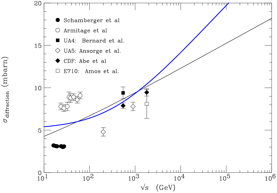


References
- [1] L. Durand and H. Pi, Phys. Rev. D 38, 78 (1988).
- [2] T. K. Gaisser and F. Halzen, Phys. Rev. Lett. 54, 1754 (1985).
- [3] G. Pancheri and Y. Srivastava, Phys. Lett. B159, 69 (1985).
- [4] M. L. Good and W. D. Walker, Phys. Rev. 120, 1857 (1960).
- [5] A. B. Kaidalov, Phys. Rept. 50, 157 (1979).
- [6] R. S. Fletcher, Phys. Rev. D 46, 187 (1992).
- [7] S. Roesler, R. Engel and J. Ranft, Z. Phys. C 59, 481 (1993).
- [8] M. G. Ryskin, A. D. Martin and V. A. Khoze, Eur. Phys. J. C 54, 199 (2008) [arXiv:0710.2494 [hep-ph]].
- [9] E. Gotsman, E. Levin, U. Maor and J. S. Miller, Eur. Phys. J. C 57, 689 (2008) [arXiv:0805.2799 [hep-ph]].
- [10] H. I. Miettinen and J. Pumplin, Phys. Rev. D 18, 1696 (1978).
- [11] E. J. Ahn, R. Engel, T. K. Gaisser, P. Lipari and T. Stanev, arXiv:0906.4113 [hep-ph].
- [12] M. Burkardt, Int. J. Mod. Phys. A 18, 173 (2003) [arXiv:hep-ph/0207047].
- [13] M. Diehl, Phys. Rept. 388, 41 (2003) [arXiv:hep-ph/0307382].
- [14] A. V. Belitsky and A. V. Radyushkin, Phys. Rept. 418, 1 (2005) [arXiv:hep-ph/0504030].
- [15] T. Sjostrand and M. van Zijl, Phys. Rev. D 36, 2019 (1987).
- [16] T. Sjostrand, S. Mrenna and P. Skands, JHEP 0605, 026 (2006) [arXiv:hep-ph/0603175].
- [17] M. Bahr, S. Gieseke and M. H. Seymour, JHEP 0807, 076 (2008) [arXiv:0803.3633 [hep-ph]].
- [18] M. Bahr, J. M. Butterworth and M. H. Seymour, JHEP 0901, 065 (2009) [arXiv:0806.2949 [hep-ph]].
- [19] D. E. Acosta et al. [CDF Collaboration], Phys. Rev. D 70, 072002 (2004) [arXiv:hep-ex/0404004].
- [20] A. A. Affolder et al. [CDF Collaboration], Phys. Rev. D 65, 092002 (2002).
- [21] M. M. Block and R. N. Cahn, Rev. Mod. Phys. 57, 563 (1985).
- [22] L. Durand and H. Pi, Phys. Rev. D 40, 1436 (1989).
- [23] N. A. Amos et al., Nucl. Phys. B 262, 689 (1985).
- [24] G. Arnison et al. [UA1 Collaboration], Phys. Lett. B 128, 336 (1983).
- [25] C. Avila et al. [E811 Collaboration], Phys. Lett. B 445, 419 (1999).
- [26] F. Abe et al. [CDF Collaboration], Phys. Rev. D 50, 5550 (1994).
- [27] F. Abe et al. [CDF Collaboration], Phys. Rev. D 50, 5518 (1994).
- [28] J. Dias de Deus and J. Kwiecinski, Phys. Lett. B 196, 537 (1987).
- [29] B. Margolis, P. Valin, M. M. Block, F. Halzen and R. S. Fletcher, Phys. Lett. B 213, 221 (1988).
- [30] A. Capella, U. Sukhatme, C. I. Tan and J. Tran Thanh Van, Phys. Rept. 236, 225 (1994).
- [31] K. Werner, Phys. Rept. 232, 87 (1993).
- [32] R. S. Fletcher, T. K. Gaisser, P. Lipari and T. Stanev, Phys. Rev. D 50, 5710 (1994).
- [33] R. M. Godbole, A. Grau, G. Pancheri and Y. N. Srivastava, Phys. Rev. D 72, 076001 (2005) [arXiv:hep-ph/0408355].
- [34] U. Amaldi, M. Jacob and G. Matthiae, Ann. Rev. Nucl. Part. Sci. 26, 385 (1976).
- [35] S. Sapeta, Phys. Lett. B 597, 352 (2004) [arXiv:hep-ph/0407038].
- [36] S. Sapeta and K. J. Golec-Biernat, Phys. Lett. B 613, 154 (2005) [arXiv:hep-ph/0502229].
- [37] F. Abe et al. [CDF Collaboration], Phys. Rev. D 50, 5535 (1994).
- [38] N. A. Amos et al. [E710 Collaboration], Phys. Lett. B 301, 313 (1993).
- [39] M. Gluck, E. Reya and A. Vogt, Z. Phys. C 67, 433 (1995).
- [40] P. M. Nadolsky et al., Phys. Rev. D 78, 013004 (2008) [arXiv:0802.0007 [hep-ph]].
- [41] A. D. Martin, R. G. Roberts, W. J. Stirling and R. S. Thorne, Eur. Phys. J. C 4, 463 (1998) [arXiv:hep-ph/9803445].
- [42] A. D. Martin, W. J. Stirling, R. S. Thorne and G. Watt, arXiv:0901.0002 [hep-ph].
- [43] J. R. Cudell et al. [COMPETE Collaboration], Phys. Rev. Lett. 89, 201801 (2002) [arXiv:hep-ph/0206172].
- [44] W. M. Yao et al. [Particle Data Group], J. Phys. G 33, 1 (2006).
- [45] R. D. Schamberger, J. Lee-Franzini, R. Mccarthy, S. Childress and P. Franzini, Phys. Rev. Lett. 34, 1121 (1975).
- [46] J. C. M. Armitage et al., Nucl. Phys. B 194, 365 (1982).
- [47] D. Bernard et al. [UA4 Collaboration], Phys. Lett. B 186, 227 (1987).
- [48] R. E. Ansorge et al. [UA5 Collaboration], Z. Phys. C 33, 175 (1986).