Deterministic Algorithms for the Lovász Local Lemma
Abstract
The Lovász Local Lemma [7] (LLL) is a powerful result in probability theory that informally states the following: the probability that none of a set of bad events happens is positive if the probability of each event is small compared to the number of events that depend on it. The LLL is often used for non-constructive existence proofs of combinatorial structures. A prominent application is to -CNF formulas, where the LLL implies that if every clause in a formula shares variables with at most other clauses then such a formula has a satisfying assignment. Recently, a randomized algorithm to efficiently construct a satisfying assignment in this setting was given by Moser [17]. Subsequently Moser and Tardos [18] gave a general algorithmic framework for the LLL and a randomized algorithm within this framework to construct the structures guaranteed by the LLL. The main problem left open by Moser and Tardos was to design an efficient deterministic algorithm for constructing structures guaranteed by the LLL. In this paper we provide such an algorithm. Our algorithm works in the general framework of Moser–Tardos with a minimal loss in parameters. For the special case of constructing satisfying assignments for -CNF formulas with clauses, where each clause shares variables with at most other clauses, for any , we give a deterministic algorithm that finds a satisfying assignment in time . This improves upon the deterministic algorithms of Moser and of Moser–Tardos with running times and respectively, which are super-polynomial for and , and upon the previous best deterministic algorithm of Beck which runs in polynomial time only for . Our algorithm is the first deterministic algorithm that works in the general framework of Moser–Tardos. We also give a parallel NC algorithm for the same setting improving upon an algorithm of Alon [1].
1 Introduction
The Lovász Local Lemma [7] (henceforth LLL) informally states that the probability that none of a set of bad events happens is nonzero if the probability of each event is small compared to the number of events that depend on it (see Section 1.1 for details). It is a powerful result in probability theory and is often used in conjunction with the probabilistic method to prove the existence of combinatorial structures. For this, one designs a random process guaranteed to generate the desired structure if none of a set of bad events happens. If the events satisfy the above-mentioned condition, then the LLL guarantees that the probability that the random process builds the desired structure is positive, thereby implying its existence. For many applications of the LLL, it is also important to find the desired structures efficiently. Unfortunately, the original proof of the LLL [7] does not lead to an efficient algorithm. In many applications of the LLL, the probability of none of the bad events happening is negligible. Consequently, the same random process does not directly provide a randomized algorithm to find the desired structure. Further, in most applications where the LLL is useful (e.g., [9, 12, 14]), the proof of existence of the desired structure is known only through the LLL (one exception to this is [9]). Thus, an efficient algorithm for the LLL would also lead to an efficient algorithm to find these desired structures. Starting with the work of Beck [3], a number of papers, e.g. [1, 5, 15, 21, 16], have sought to make the LLL algorithmic. Before discussing these results in more detail we describe the LLL formally.
1.1 The Lovász Local Lemma
The Lovász Local Lemma gives a lower bound on the probability of avoiding a possibly large number of “bad” events that are not “too dependent” on each other. Let be a finite set of events in a probability space. Let be an undirected graph on vertex set with the property that every event is mutually independent11 1 An event is mutually independent of a set of events if for every function that can be expressed using finitely many unions and intersections of the arguments. of the set of all events not in its neighborhood. We assume throughout that does not contain any self-loops. We denote the set of neighbors of an event by , i.e., . The general version of the LLL is the following.
Theorem 1.
A simple corollary of the LLL, called symmetric LLL, often suffices in several applications. In this version there is a uniform upper bound on the probability of each event and a uniform upper bound on the number of neighbors of each event in the dependency graph. This quantity is also called the dependency degree of the event .
Corollary 2.
[7] If each event occurs with probability at most and has dependency degree such that , then the probability that none of the events occur is positive.
Proof.
Setting for all events shows that the conditions of Theorem 1 are satisfied:
The power of the symmetric version is well-demonstrated by showing a satisfiability result for -CNF formulas, i.e., Boolean formulas in conjunctive normal form with variables per clause. This classic application of the LLL will help in understanding our and previous results and techniques and therefore will be a running example in the rest of the paper.
Corollary 3.
Every -CNF formula in which every clause shares variables with at most other clauses is satisfiable.
Proof.
To apply the symmetric LLL (i.e., Corollary 2) we choose the probability space to be the product space of each variable being chosen true or false independently with probability . For each clause we define an event that is said to occur if and only if clause is not satisfied. Clearly, two events and are independent unless the clauses and share variables. Now take to be the graph on the events with edges between events and iff and share variables. It is clear that each event is mutually independent of its non-neighbors in . By assumption each event has at most neighbors. Moreover, the probability that a clause is not satisfied by a random assignment is exactly . The requirement of Corollary 2 is therefore met and hence we obtain that the probability that none of the events occur is positive. The satisfiability of the -CNF formula follows.
1.2 Previous work
Algorithms for the LLL are often targeted towards one of two model problems: -CNF formula satisfiability and -uniform hypergraph 2-coloring. Interesting in their own right, these problems capture the essence of the LLL without many technicalities. Moreover, algorithms for these problems usually lead to algorithms for more general applications of the LLL [5, 14, 6]. As shown in Section 1.1, for the -CNF formula satisifiability problem, the LLL implies that every -CNF formula in which each clause shares variables with at most other clauses has a satisfying assignment. Similarly, it can be shown that the vertices of a -uniform hypergraph, in which each edge shares variables with at most other edges, can be colored using two colors so that no edge is monochromatic. The algorithmic objective is to efficiently find such a 2-coloring (or a satisfying assignment in the case of -CNF).
This question was first addressed by Beck in his seminal paper [3], where he gave an algorithm for the hypergraph 2-coloring problem with dependency degree . More precisely, he gave a polynomial-time deterministic algorithm to find a 2-coloring of the vertices of every -uniform hypergraph in which each edge shares vertices with other edges such that no edge is monochromatic. Molloy and Reed [14] showed that the dependency degree of this algorithm can be improved to . In the same volume in which Beck’s paper appeared, Alon [1] gave a randomized parallel version of Beck’s algorithm that outputs a valid 2-coloring when the dependency degree is at most and showed that this algorithm can be derandomized22 2 Alon did not attempt to optimize the exponent but Srinivasan [21] states that optimizing the bound would still lead to an exponent with several tens in the denominator.. Since then, tremendous progress has been made on randomized LLL algorithms. Nonetheless, prior to our work, Beck’s and Alon’s algorithms remained the best deterministic and parallel algorithms for the (symmetric) LLL.
For randomized algorithms and algorithms that require to be a fixed constant, a long line of work improved the maximum achievable dependency degree and the generality of the results culminating in the work of Moser and Tardos [18]. Moser and Tardos [18] provided a simple randomized (parallel) algorithm for the general LLL. These results are summarized in Table 1, and we discuss them next.
| Max. Dep. Deg. | Det. | Par. | Remark | |
|---|---|---|---|---|
| Beck [3] | X | |||
| Beck [14] | X | prev. best det. algorithm | ||
| Alon [1] | X | X | prev. best det. par. algorithm | |
| X | X | only for constant k,d | ||
| Srinivasan [21] | ||||
| X | ||||
| Moser [16] | ||||
| X | only for constant k,d | |||
| Moser [17] | ||||
| X | only for constant k,d | |||
| Moser, Tardos [18] | ||||
| X | ||||
| X | X | only for constant k,d | ||
| Our work | X | X |
Alon [1] gave an algorithm that is efficient for a dependency degree of if one assumes that and therefore also the dependency degree is bounded above by a fixed constant. Molloy and Reed [15] generalized Alon’s method to give efficient algorithms for a certain set-system model for applications of the symmetric form of the LLL. Czumaj and Scheideler [5, 6] consider the algorithmic problem for the asymmetric version of the LLL. The asymmetric version of the LLL addresses the possibility of 2-coloring the vertices of non-uniform hypergraphs with no monochromatic edges. The next improvement in increasing the dependency degree threshold was due to Srinivasan [21]. He gave a randomized algorithm for hypergraph 2-coloring when the dependency degree is at most . Moser [16] improved the dependency degree threshold to using a variant of Srinivasan’s algorithm. Later, Moser [17] achieved a significant breakthrough improving the dependency degree threshold to using a much simpler randomized algorithm. Moser and Tardos [18] closed the small constant-factor gap to the optimal dependency degree guaranteed by the general LLL.
More importantly, Moser–Tardos [18] gave an algorithmic framework for the general version of the LLL (discussed in Section 2.1) that minimally restricts the abstract LLL setting to make it amenable for algorithmic considerations. In this framework they gave an efficient randomized algorithm for computing the structures implied by the LLL. The importance of the framework stems from the fact that it captures most of the LLL applications, thus directly providing algorithms for these applications. Moser [16, 17] and Moser–Tardos [18] also gave a derandomization of their algorithms obtaining an algorithm that runs in time, where is the maximum dependency degree and is the number of events. For the simpler -CNF problem, the running time of the deterministic algorithms can be improved to . Nonetheless, this running time is polynomial only under the strong condition that and the dependency degree are bounded by a fixed constant.
The main open question that remained open was to obtain deterministic algorithms that go beyond the initial results of Beck [3] and that are efficient for unbounded dependency degrees. We address this question by giving new derandomizations of the Moser–Tardos algorithm. We give a derandomization that works efficiently for the general version of the LLL in the aforementioned algorithmic framework of Moser–Tardos [18] assuming a mild -slack in the LLL conditions. As a corollary, we obtain an algorithm that runs in time to find a satisfying assignment for a -CNF formula with clauses such that no clause shares variables with more than other clauses, for any . We note that our -slack assumption is in the exponent as opposed to the multiplicative slackness in the Moser–Tardos results (see Table 1). We also extend the randomized parallel algorithm of Moser–Tardos to obtain an efficient deterministic parallel algorithm under the same assumption thereby improving over Alon’s algorithm with a dependency degree of .
Organization. In Section 2, we describe the algorithmic framework of Moser–Tardos for the LLL and their algorithm. In Section 3, we state our results and their implications for the -CNF problem. In Section 4, we give an informal description of the new ideas in the paper. In Section 5, we formally define the major ingredient in our derandomization: the partial witness structure. In Section 6, we give our sequential deterministic algorithm and analyze its running time. Finally, in Section 7, we present our parallel algorithm and its running time analysis.
2 Preliminaries
2.1 Algorithmic Framework
To get an algorithmic handle on the LLL, we move away from the abstract probabilistic setting of the original LLL. We impose some restrictions on the representation and form of the probability space under consideration. In this paper we follow the algorithmic framework for the LLL due to Moser–Tardos [18]. We describe the framework in this section.
The probability space is given by a finite collection of mutually independent discrete random variables . Let be the domain of , which is assumed to be finite. Every event in a finite collection of events is determined by a subset of . We define the variable set of an event as the unique minimal subset that determines and denote it by .
The dependency graph of the collection of events is a graph on vertex set . The graph has an edge between events , if . For we denote the neighborhood of in by and define . Note that events that do not share variables are independent.
It is useful to think of as a family of “bad” events. The objective is to find a point in the probability space, or equivalently, an evaluation of the random variables from their respective domains, for which none of the bad events happens. We call such an evaluation a good evaluation.
2.2 The Moser–Tardos Algorithm
Moser-Tardos [18] presented the very simple Algorithm 1 to find a good evaluation.
Algorithm 1:
Sequential Moser–Tardos Algorithm
- 1.
For every , a random evaluation of .
- 2.
While such that happens on the current evaluation , do
- (a)
Pick one such that happens (any arbitrary choice would work).
- (b)
Resample : For all , do
- •
a new random evaluation of .
- •
- (a)
- 3.
Return .
Observe that if the algorithm terminates, then it outputs a good evaluation. The following theorem from [18] shows that the algorithm is efficient if the LLL-conditions are met.
3 Results
This section formally states the new results established in this paper.
If an assignment of reals as stated in Theorem 4 exists, then we use such an assignment to define the following parameters33 3 Throughout this paper denotes the logarithm to base .:
- •
.
- •
.
- •
.
- •
.
- •
.
For the rest of this paper, we will use these parameters to express the running time of our algorithms.
Our sequential deterministic algorithm assumes that for every event , the conditional probability of occurrence of under any partial assignment to the variables in , can be computed efficiently. This is the same complexity assumption as used in Moser–Tardos [18]. It can be further weakened to use pessimistic estimators.
Theorem 5.
Let the time needed to compute the conditional probability for any and any partial evaluation , , be at most . Suppose there is an and an assignment of reals such that for all ,
Then there is a deterministic algorithm that finds a good evaluation in time
where the parameters , and are as defined above.
We make a few remarks to give a perspective for the magnitudes of the parameters involved in our running time bound. As a guideline to reading the results, it is convenient to think of as and of as .
Indeed, holds whenever the ’s are bounded away from one by a constant. For this setting we also have, without loss of generality44 4 With being bounded away from one and given the -slack assumed in our theorems one can always reduce slightly to obtain a small constant factor gap between and (similar to [18]) and then increase any extremely small to at least for some small constant . Increasing in this way only weakens the LLL-condition for the event itself. Furthermore, the effect on the LLL-condition for any event due to the changed factors of one of its (at most ) neighboring events accumulates to at most which can be made larger than the produced gap between and ., that . Lastly, the factor is usually small; e.g., in all applications using the symmetric LLL or the simple asymmetric version[15, 14] this factor is a constant. This makes at most a polynomial in and . For most applications of the LLL this also makes polynomial in the size of the input/output. For all these settings our algorithms are efficient: The running time bound of our sequential algorithm is polynomial in and that of our parallel algorithm is polylogarithmic in using at most many processors.
Notable exceptions in which is not polynomial in the input size are the problems in [10]. For these problems is still but the number of events is exponential in the number of variables and the input/output size. For these settings, the problem of checking whether a given evaluation is good is coNP-complete and obtaining a derandomized algorithm is an open question.
It is illuminating to look at the special case of -CNF both in the statements of our theorems as well as in the proofs, as many of the technicalities disappear while retaining the essential ideas. For this reason, we state our results also for -CNF. The magnitudes of the above parameters in the -CNF applications are given by , , , and .
Corollary 6.
For any there is a deterministic algorithm that finds a satisfying assignment to any -CNF formula with clauses in which each clause shares variables with at most other clauses in time .
We also give a parallel deterministic algorithm. This algorithm makes a different complexity assumption about the events, namely, that their decision tree complexity is small. This assumption is quite general and includes almost all applications of the LLL (except again for the problems mentioned in [10]). They are an interesting alternative to the assumption that conditional probabilities can be computed efficiently as used in the sequential algorithm.
Theorem 7.
For a given evaluation, let the time taken by processors to check the truth of an event be at most . Let be the time to compute the maximal independent set in an -vertex graph using parallel processors on an EREW PRAM. Suppose, there is an and an assignment of reals such that for all ,
If there exists a constant such that every event has decision tree complexity55 5 Informally, we say that a function has decision tree complexity at most if we can determine its value by adaptively querying at most of the input variables. at most , then there is a parallel algorithm that finds a good evaluation in time
using processors.
The fastest known algorithm for computing the maximal independent set in an -vertex graph using parallel processors on an EREW PRAM runs in time [2, 13]. Using this in the theorem, we get the following corollary for -CNF.
Corollary 8.
For any there is a deterministic parallel algorithm that uses processors on an EREW PRAM and finds a satisfying assignment to any -CNF formula with clauses in which each clause shares variables with at most other clauses in time .
4 Techniques
In this section, we informally describe the main ideas of our approach in the special context of -CNF formulas and indicate how they generalize. Reading this section is not essential but provides intuition behind the techniques used for developing deterministic algorithms for the general LLL. For the sake of exposition in this section, we omit numerical constants in some mathematical expressions. Familiarity with the Moser–Tardos paper [18] is useful but not necessary for this section.
4.1 The Moser–Tardos Derandomization
Let be a -CNF formula with clauses. We note immediately that if , then the probability that a random assignment does not satisfy a clause is . Thus the probability that on a random assignment, has an unsatisfied clause is at most , and hence a satisfying assignment can be found in polynomial time using the method of conditional probabilities (see, e.g., [14]). Henceforth, we assume that . We also assume that each clause in shares variables with at most other clauses; thus the LLL guarantees the existence of a satisfying assignment.
To explain our techniques we first need to outline the deterministic algorithms of Moser and of Moser–Tardos which work in polynomial time, albeit only for . Consider a table of values: for each variable in the table has a sequence of values, each picked at random according to its distribution. We can run Algorithm 1 using such a table: instead of randomly sampling afresh each time a new evaluation for a variable is needed, we pick its next unused value from . The fact that the randomized algorithm terminates quickly in expectation (Theorem 4), implies that there exist small tables (i.e., small lists for each variable) on which the algorithm terminates with a satisfying assignment. The deterministic algorithm finds one such table.
The constraints to be satisfied by such a table can be described in terms of witness trees: for a run of the randomized algorithm, whenever an event is resampled, a witness tree “records” the sequence of resamplings that led to the current resampling. We will not define witness trees formally here; see [18] or Section 5 for a formal definition. We say that a witness (we will often just use “witness” instead of “witness tree”) is consistent with a table, if this witness arises when the table is used to run Algorithm 1. If the algorithm using a table does not terminate after a small number of resamplings, then it has a large consistent witness certifying this fact. Thus if we use a table which has no large consistent witness, the algorithm should terminate quickly.
The deterministic algorithms of Moser and of Moser–Tardos compute a list of witness trees satisfying the following properties.
- 1.
Consider an arbitrary but fixed table . If no witness in is consistent with , then there is no large witness tree consistent with .
- 2.
The expected number of witnesses in consistent with a random table is less than . This property is needed in order to apply the method of conditional probabilities to find a small table with which no tree in is consistent.
- 3.
The list is of polynomial size. This property is necessary for the method of conditional probabilities to be efficient.
We now describe how these properties arise naturally while using Algorithm 1 and how to find the list . In the context of -CNF formulas with clauses satisfying the degree bound, Moser (and also Moser–Tardos when their general algorithm is interpreted for -CNF) prove two lemmas that they use for derandomization. The expectation lemma states that the expected number of large (size at least ) consistent witness trees (among all possible witness trees) is less than (here randomness is over the choice of the table). At this point we could try to use the method of conditional probabilities to find a table such that there are no large witness trees consistent with it. However there are infinitely many witness trees, and so it is not clear how to proceed by this method.
This difficulty is resolved by the range lemma which states that if for some , no witness tree with size in the range is consistent with a table, then no witness tree of size at least is consistent with the table. Thus, the list is the set of witness trees of size in the range . Now one can find the required table by using the method of conditional probabilities to exclude all tables with a consistent witness in . The number of witnesses in is . To proceed by the method of conditional probabilities we need to explicitly maintain and find values for the entries in the table so that none of the witnesses in remains consistent with it.
Thus, the algorithm of Moser (and respectively Moser–Tardos) works in polynomial time only for constant . Clearly, it is the size of that is the bottleneck towards achieving polynomial running time for . One possible way to deal with the large size of would be to maintain in an implicit manner, thereby using a small amount of space. We do not know how to achieve this. We solve this problem in a different way, by working with a new (though closely related) notion of witness trees, which we explain next.
4.2 Partial Witness Trees
For a run of the Moser–Tardos randomized algorithm using a table , for each resampling of an event, we get one witness tree consistent with . Given a consistent witness tree of size , removing the root gives rise to up to new consistent witnesses, whose union is the original witness minus the root. Clearly one of these new subtrees has size at least . This proves their range lemma. The range lemma is optimal for the witness trees. That is, for a given it is not possible to reduce the multiplicative factor of between the two endpoints of the range .
We overcome this limitation by introducing partial witness trees, which have properties similar to those of witness trees, but have the additional advantage of allowing a tighter range lemma. The only difference between witness trees and partial witness trees is that the root, instead of being labeled by a clause (as is the case for witness trees), is labeled by a subset of variables from . Now, instead of removing the root to construct new witness trees as in the proof of the Moser–Tardos range lemma, each subset of the set labeling the root gives a new consistent partial witness tree. This flexibility allows us to prove the range lemma for the smaller range . The number of partial witness trees is larger than the number of witness trees because there are choices for the label of the root (as opposed to choices in the case of witness trees) since the root may be labeled by any subset of variables in a clause. But , as explained at the beginning of Section 4.1. Thus for each witness tree there are at most partial witnesses and the expectation lemma holds with similar parameters for partial witnesses as well. The method of conditional probabilities now needs to handle partial witness trees of size in the range , which is the new . The number of partial witnesses in this range is , which is still too large. The next ingredient brings this number down to a manageable size.
4.3 -slack
By introducing an -slack, that is, by making the slightly stronger assumption that each clause intersects at most other clauses, we can prove a stronger expectation lemma: The expected number of partial witnesses of size more than is less than . Indeed, the number of labeled trees of size and degree at most is less than (see [11]). Thus the number of partial witnesses of size is less than , where the factor () accounts for the number of possible labels for the root. Moreover, the probability that a given partial witness tree of size is consistent with a random table is (as opposed to in the case of a witness tree). This is proved in a similar manner as for witness trees. Thus the expected number of partial witnesses of size at least consistent with a random table is at most
Now, by the new expectation and range lemmas it is sufficient to consider partial witnesses of size in the range . The number of partial witnesses of size in this range is polynomial in ; thus the list of trees that the method of conditional probabilities needs to maintain is polynomial in size.
4.4 General Version
More effort is needed to obtain a deterministic algorithm for the general version of the LLL. Here, the events are allowed to have significantly varying probabilities of occurrence and unrestricted structure.
One issue is that an event could possibly depend on all variables. In that case, taking all variable subsets of a label for the root of a partial witness would give up to different possible labels for the roots. However, for the range lemma to hold true, we do not need to consider all possible variable subsets for the root; instead, for each root event it is sufficient to have a pre-selected choice of labels. This pre-selected choice of labels is fixed for each event in the beginning.
The major difficulty in derandomizing the general LLL is in finding a list satisfying the three properties mentioned earlier for applying the method of conditional probabilities. The range lemma can still be applied. However, the existence of low probability events with (potentially) many neighbors may lead to as many as partial witnesses of size in the range . Indeed, it can be shown that there are instances in which there is no setting of such that the list containing all witnesses of size in the range satisfies properties (2) and (3) mentioned in Section 4.1.
The most important ingredient for working around this in the general setting is the notion of weight of a witness tree. The weight of a tree is the sum of the weights of individual vertices; more weight is given to those vertices whose corresponding bad events have smaller probability of occurrence. Our deterministic algorithm for the general version finds a list that consists of partial witnesses with weight (as opposed to size) in the range , where is a number depending on the problem. It is easy to prove a similar range lemma for weight based partial witnesses which guarantees property (1) for this list. Further, the value of can be chosen so that the expectation lemma of Moser and Tardos can be adjusted to lead to property (2) for . Unfortunately one cannot prove property (3) by counting the number of partial witnesses using combinatorial enumeration methods as in [17]. This is due to the possibility of up to neighbors for each event in the dependency graph. However, the strong coupling between weight and probability of occurrence of bad events can be used to obtain property (3) directly from the expectation lemma.
4.5 Parallel Algorithm
For the parallel algorithm, we use the technique of limited-independence spaces, or more specifically -wise -dependent probability spaces due to Naor and Naor[19] and its extensions [8, 4]. This is a well-known technique for derandomization. The basic idea here is that instead of using perfectly random bits in the randomized algorithm, we use random bits chosen from a limited-independence probability space. For many algorithms it turns out that their performance does not degrade when using bits from such a probability space; but now the advantage is that these probability spaces are much smaller in size and so one can enumerate all the sample points in them and choose a good one, thereby obtaining a deterministic algorithm. This tool was applied by Alon [1] to give a deterministic parallel algorithm for -uniform hypergraph 2-coloring and other applications of the LLL, but with much worse parameters than ours. Our application of this tool is quite different from the way Alon uses it: Alon starts with a random 2-coloring of the hypergraph chosen from a small size limited independence space; he then shows that at least one of the sample points in this space has the property that the monochromatic hyperedges and almost monochromatic hyperedges form small connected components. For such a coloring, one can alter it locally over vertices in each component to get a valid 2-coloring.
In contrast, our algorithm is very simple (we describe it for -CNF; the arguments are very similar for hypergraph 2-coloring and for the general LLL): recall that for a random table, the expected number of consistent partial witnesses with size in the range is at most (for the case of -CNF). Each of these partial witnesses uses at most entries from the table. Now, instead of using a completely random table, we use a table chosen according to a -wise independent distribution (i.e., any subset of at most entries has the same joint distribution as in a random table). So any partial witness tree is consistent with the new random table with the same probability as before. And hence the expected number of partial witnesses consistent with the new random table is still at most . But now the key point to note is that the number of tables in the new limited independence distribution is much smaller and we can try each of them in parallel until we succeed with one of the tables. To make the probability space even smaller we use -wise -dependent distributions, but the idea remains the same. Finally, to determine whether a table has no consistent partial witness whose size is at least , we run the parallel algorithm of Moser–Tardos on the table.
In order to apply the above strategy to the general version, we require that the number of variables on which witnesses depend be small, and hence the number of variables on which events depend should also be small. In our general parallel algorithm we relax this to some extent: instead of requiring that each event depend on few variables, we only require that the decision tree complexity of the event be small. The idea behind the proof remains the same.
5 The Partial Witness Structure
In this section we define the partial witness structure and their weight. We then prove the new range lemma using these weights.
5.1 Definitions
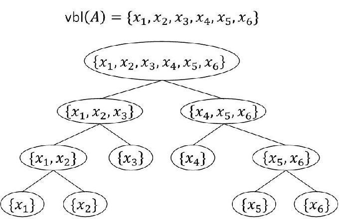
For every we fix an arbitrary rooted binary variable splitting . It is a binary tree in which all vertices have labels which are nonempty subsets of : The root of is labeled by itself, the leaves are labeled by distinct singleton subsets of and every non-leaf vertex in is labeled by the disjoint union of the labels of its two children. This means that every non-root non-leaf vertex is labeled by a set , while its children are labeled by and for some . Note that consists of vertices. We abuse the notation to also denote the set of labels of the vertices of this binary variable splitting. The binary variable splitting is not to be confused with the (partial) witness tree which we define next. The elements from will solely be used to define the possible labels for the roots of partial witness trees. An example of a binary variable splitting can be found in Figure 1.
A partial witness tree is a finite rooted tree whose vertices apart from the root are labeled by events from while the root is labeled by some subset of variables with for some . Each child of the root must be labeled by an event that depends on at least one variable in (thus a neighbor of the corresponding root event); the children of every other vertex that is labeled by an event must be labeled either by or by a neighboring event of , i.e., its label should be from . Define to be the set of vertices of . For notational convenience, we use and denote the label of a vertex by .
A full witness tree is a special case of a partial witness where the root is the complete set for some . In such a case, we relabel the root with instead of . Note that this definition of a full witness tree is the same as the one of the witness trees in [18].
Define the weight of an event to be . Define the weight of a partial witness tree as the sum of the weights of the labels of the vertices in , i.e.,
The depth of a vertex in a witness tree is the distance of from the root in the witness tree. We say that a partial witness tree is proper if for every vertex , all children of have distinct labels.
Similar to [16], we will control the randomness used by the algorithm using a table of evaluations, denoted by . It is convenient to think of as a matrix. This table contains one row for each variable in . Each row contains evaluations for its variable. Note that the number of columns in the table could possibly be infinite. In order to use such a table in the algorithm, we maintain a pointer for each variable indicating the column containing its current value used in the evaluation of the events. We denote the value of at by . If we want to resample an evaluation for , we increment the pointer by one, and use the value at the new location.
We call a table a random table if, for all variables and all positions , the entry is picked independently at random according to the distribution of . It is clear that running Algorithm 1 is equivalent to using a random table to run Algorithm 2 below.
Algorithm 2:
Moser-Tardos Algorithm with input table
Input: Table with values for variables
Output: An assignment of values for variables so that none of the events in happens
- 1.
For every variable : Initialize the pointer .
- 2.
While that happens on the current assignment (i.e., ) do
- (a)
Pick one such .
- (b)
Resample : For all increment by one.
- (a)
- 3.
Return .
In the above algorithm, Step 2(a) is performed by a fixed arbitrary deterministic procedure. This makes the algorithm well-defined.
Let be an ordering of the events (with repetitions), which we call the event-log. Let the ordering of the events as they have been selected for resampling in the execution of Algorithm 2 using a table be denoted by an event-log . Observe that is partial if the algorithm terminates after a finite number of resamplings ; i.e., is defined only for .
Given an event-log , associate with each resampling step and each , a partial witness tree as follows. Define to be an isolated root vertex labeled . Going backwards through the event-log, for each : (i) if there is a non-root vertex such that , then among all such vertices choose the one whose distance from the root is maximum (break ties arbitrarily) and attach a new child vertex to with label , thereby obtaining the tree , (ii) else if is non-empty, then attach a new child vertex to the root with label to obtain , (iii) else, set . Finally set .
Note that if then is a full witness tree with root . For such a full witness tree, our construction is the same as the construction of witness trees associated with the log in [18].
We say that the partial witness tree occurs in event-log if there exists such that for some such that , and . An illustrating example of these definitions can be found in Figure 2.
 |
 |
| Dependency graph | Partial witness tree |
For a table , a -check on a partial witness tree uses table as follows: In decreasing order of depth, visit the non-root vertices of and for a vertex with label , take the first unused value from for each and check if the resulting evaluation makes happen. The -check passes if all events corresponding to vertices apart from the root, happen when checked. We say that a partial witness tree is consistent with a table if the -check passes on the partial witness tree.
Most of the above definitions are simple extensions of the ones given in [18].
5.2 Properties
In this section we state and prove two important properties of the partial witness tree which will be useful in obtaining the deterministic sequential and parallel algorithms.
The following lemma proves that given a witness tree, one can use the -check procedure to exactly determine which values were used in the resamplings that lead to this witness tree.
Lemma 9.
For a fixed table , if a partial witness tree occurs in the event-log , then
- 1.
is proper.
- 2.
is consistent with .
Proof.
The proof of this lemma is essentially Lemma 2.1 in [18] and included here for completeness.
Since occurs in , there exists some time instant such that for , . For each , let denote the depth of vertex and let denote the largest value with contained in . We observe that is the time instant in which was attached to by the procedure constructing .
If for vertices and and are not disjoint, then . Indeed, when adding the vertex to we attach it to or to another vertex of equal or greater depth. Therefore, for any two vertices at the same depth , and do not depend on any common variables, that is the labels in every level of form an independent set in . In particular must be proper.
Now consider a non-root vertex in the partial witness tree . Let . Let be the set of vertices with depth greater than that of such that depends on variable .
When the -check considers the vertex and uses the next unused evaluation of the variable , it uses the evaluation . This is because the witness check visits the vertices in order of decreasing depth and among the vertices with depth equal to that of , only depends on (as we proved earlier that vertices with equal depth are variable disjoint). So the -check must have used values for exactly when it was considering the vertices in .
At the time instant of resampling , say , Algorithm 2 chooses to be resampled which implies that happens before this resampling. For , the value of the variable at is . This is because the pointer for was increased for events that were resampled before the current instance, where . Note that every event which was resampled before and that depends on would be present at depth greater than that of in by construction. Hence, is the complete set of events which led to resampling of before the instant .
As the -check uses the same values for the variables in when considering as the values that led to resampling of , it must also find that happens.
Next, we prove a range lemma for partial witnesses, improving the range to a factor of two.
Lemma 10.
If a partial witness tree of weight at least occurs in the event-log and every vertex in the tree has weight at most , then a partial witness tree of weight occurs in the event-log .
Proof.
The proof is by contradiction. Consider a least weight partial witness tree whose weight is at least that occurs in the event-log , namely for some , where . A witness tree with weight at least exists by assumption and because there are only finitely many choices for and there exists also a least weight such tree. Suppose, for the sake of contradiction, that . We may assume that Root has at least one child, otherwise, the weight of the tree is zero. We have two cases:
Case (i): Root has only one child . Let be the largest time instant before at which was resampled. Note that this resampling of corresponds to the child of the root of . Now, consider the partial witness tree . Since contains one less vertex than , . Also, since the weight of any vertex in the tree is at most we get that . Finally, by definition of , it is clear that occurs in the event-log . Thus, is a counterexample of smaller weight contradicting our choice of .
Case (ii): Root has at least two children. Since the labeling clauses of these children have pairwise disjoint sets of variables and they have to share a variable with , we have that consists of at least variables. Thus, it also has at least two children in the variable splitting . In , starting from , we now explore the descendants of in the following way, looking for the first vertex whose children and reduce the weight of the tree, i.e., , where and : if a vertex reduces the weight of the tree without making it zero (i.e., ), then its variable disjoint sibling must also reduce the weight of the tree; on the other hand, if a vertex reduces the weight of the tree to zero, then its sibling cannot reduce the weight of the tree. Suppose reduces the weight to zero, then we explore to check if its children reduce the weight. It is easy to see that this stops at the latest when and are leaves in .
By definition, both and occur in the event-log . Since we pick the first siblings and (in the breadth first search) which reduce the weight, their parent is such that , where . We are considering only those such that . This implies that . Hence, and for every vertex that has label in , one can find a unique vertex labeled by in and vice-versa. Further, is the disjoint union of and ; therefore, for each vertex with label in , one can find a unique vertex labeled by either in or .
As a consequence, we have that for every vertex with label in , one can find a unique vertex labeled by either in or . Hence, and therefore, . So, the witness with larger weight among and has weight at least but less than that of . This contradicts our choice of .
6 Deterministic Algorithm
In this section we describe our sequential deterministic algorithm and prove Theorem 5.
For the rest of the paper we define a set of forbidden witnesses which contains all partial witness trees with weight between and . We define a table to be a good table if no forbidden witness is consistent with it. With these definitions we can state our deterministic algorithm.
Algorithm 3:
Sequential Deterministic Algorithm
- 1.
Enumerate all forbidden witnesses in .
- 2.
Construct a good table via the method of conditional probabilities:
For each variable , and for each , , do- •
Select a value for that minimizes the expected number of forbidden witnesses that are consistent with when all entries in the table chosen so far are fixed and the yet to be chosen values are random.
- •
- 3.
Run Algorithm 2 using table as input.
We next give a short overview of the running time analysis of Algorithm 3 before embarking on the proof of Theorem 5.
The running time of Algorithm 3 depends on the time to construct a good table by the method of conditional probabilities. To construct such a table efficiently, we prove that the number of forbidden witnesses is small (polynomial in ) using Lemma 12. Further, we need to show that the method of conditional probabilities indeed constructs a good table. We show this by proving in Lemma 11 that the expected number of forbidden witnesses that are consistent with initially (when all values are random) is smaller than one. This invariant is maintained by the method of conditional probabilities resulting in a fixed table with less than one (and therefore no) forbidden witnesses consistent with it. By Lemmas 9 and 10, it follows that no witness of weight more than occurs when Algorithm 2 is run on the table . Finally, the maximum number of vertices in a partial witness tree of weight at most is small. This suffices to show that the size of table is small and thus Algorithm 3 is efficient.
Lemma 11.
The expected number of forbidden witnesses consistent with a random table is less than .
Proof.
For each event , let and be the set of partial and respectively full witness trees in with root from . With this notation the expectation in question is exactly:
Note that according to Lemma 9, a partial witness tree is consistent with a table if and only if it passes the -check. Clearly, the probability that a witness passes the -check for the random table is (recall that denotes the set of non-root vertices in ). Using this and the assumption in Theorem 5 that we get that the expectation is at most
To relate this to the full witness trees considered in [18], we associate with every partial witness tree (in ) a full witness tree (in ) by replacing the root subset with the full set . Note that the weights of and are the same (as is the quantity ). Note also that every full witness tree has at most partial witness trees associated with it. Hence, we can rewrite the expression to get
where the last expression follows because, for , we have
Next we transition from partial to full witness trees by including the root again (and going from to ).
Now we can use the following result of Moser–Tardos (Section 3 in [18]) that bounds the expected number of full witnesses with root :
Their proof makes use of a Galton–Watson process that randomly generates proper witness trees with root (note that by Lemma 9 all partial witness trees are proper). Using this,
Here the penultimate inequality follows from the fact that and the definition of , and the last inequality follows from the choice of .
Owing to the definition of forbidden witnesses via weights, there is an easy way to count the number of forbidden witnesses using the fact that their expected number is small.
Lemma 12.
The number of witnesses with weight at most is at most . In particular, the number of forbidden witnesses is less than .
Proof.
Each forbidden witness has weight and thus
Here, the final line of inequalities comes from the proof of Lemma 11. Therefore the number of forbidden witnesses is at most
Using the same argument with any instead of shows that the number of witnesses with weight in is at most . Since this is exponential in the total number of witnesses with weight at most is dominated by a geometric sum which is .
We are now ready to prove Theorem 5.
Proof of Theorem 5.
We first describe how the set of forbidden witnesses in the first step of the deterministic algorithm (Algorithm 3) is obtained.
Enumeration of witnesses.
We enumerate all witnesses of weight at most and then discard the ones with weight less than . According to Lemma 12, there are at most witnesses of weight at most and each of them consists of at most vertices. In our discussion so far we did not need to consider the order of children of a node in our witness trees. However, for the enumeration it will be useful to order the children of each node from left to right. We will build witnesses by attaching nodes level-by-level and from left to right. We fix an order on the events according to their weights, breaking ties arbitrarily, and use the convention that all witnesses are represented so that for any node its children from left to right have increasing weight. We then say a node is eligible to be attached to a witness if in the resulting witness the node is the deepest rightmost leaf in . With this convention the enumeration proceeds as follows:
As a preprocessing step for every event we sort all the events in according to their weight in time. Then, starting with , the set of all possible roots, we incrementally compute all witnesses having nodes and weight at most . To obtain from we take each witness and each node and check for all with weight more than the current children of , in the order of increasing weight whether a node with is eligible to be attached to at . If it is eligible, and the resulting new witness has weight at most , then we add to . It is clear that in this way we enumerate all forbidden witnesses without producing any witness more than once.
We now analyze the time required by the above enumeration procedure. We write down each witness explicitly, taking time and space per witness. For each witness it takes linear (in the number of nodes) time to find the nodes with eligible children. Note that attaching children to a node in the order of increasing weight guarantees that at most one attachment attempt per node fails due to large weight. Thus, the total time to list all forbidden witnesses is at most .
Finding a good table.
The running time to find a good table using the method of conditional probabilities as described in Algorithm 3 can be bounded as follows: For each of the variables, the table has entries to be filled in. For each of those entries at most possible values need to be tested. For each value we compute the conditional expectation of the number of forbidden witnesses that are consistent with the partially filled in table by computing the conditional probability of each forbidden witness to pass the -check given the filled in values and summing up these probabilities. This can be done by plugging in the fixed values into each of the at most nodes of similar to the -check procedure, computing the conditional probability in time and computing the product of these conditional probabilities. Thus, the total time to compute is at most
To complete the proof we show that the running time of the sequential algorithm on a table obtained by Step 2 of the deterministic algorithm is at most :
First, we note that by running the sequential algorithm using table , none of the forbidden witnesses can occur in the event-log . This is because the table is obtained by the method of conditional probabilities: In the beginning of the construction of the table, when no value is fixed, the expected number of forbidden witnesses that occur in the event-log is less than as proved in Lemma 11. This invariant is maintained while picking values for variables in the table. Thus, once all values are fixed, the number of witness trees in that occur in the event-log is still less than and hence zero.
This implies that the sequential algorithm with as input resamples each event at most times. Indeed, if some event is resampled more than times, then occurs in the event-log at least times. Now, the weight of the partial witness tree associated with the last instance at which was resampled, would be at least which is more than . According to Lemma 10, which is applicable since is larger than the maximum weight event, there would also be a forbidden witness of weight between and occurring in , a contradiction. Therefore, the number of resamplings done by Algorithm 2 is and the total running time for Algorithm 2 using table is : the additional factor comes from the time needed to find an event that happens. This running time is smaller than the upper bound for the time needed to find a good table .
This shows that Algorithm 3 terminates in the stated time bound. Lastly, the correctness of the algorithm follows directly from the fact that the algorithm only terminates if a good assignment is found.
From the general deterministic algorithm it is easy to obtain the corollary regarding -CNF by using the standard reduction to the symmetric LLL and plugging in the optimal values for the parameters.
Proof of Corollary 6.
For a -CNF formula with clauses , for each clause we define an event and say that the event happens if the clause is unsatisfied. Further, each variable appearing in the formula picks values uniformly at random from . Then, for every event , . As remarked in Section 4.1, we may assume that , for otherwise the problem becomes simple. If is the maximum number of clauses that a clause shares its variables with, setting for all , we obtain that . The condition that then implies for all events that as required by the LLL-condition. Therefore, we use parameters , , , and obtain . With these parameters the corollary follows directly from Theorem 5.
7 Parallel Algorithm
In this section we present an efficient parallel algorithm (outlined in Sec. 4.5) and analyze its performance, thereby proving Theorem 7.
In the design of our sequential algorithm, we used Algorithm 2 as a subroutine which takes an input table, and uses it to search for an assignment for which none of the bad events happens. This reduced the problem to finding a good input table. For designing the parallel algorithm, Moser–Tardos already provided the parallel counterpart of Algorithm 2, and so what remains is to find a good table. Our algorithm relies on the following observation: Instead of sampling the values in the table independently at random, if we choose it from a distribution that is a -approximation of the original distribution (for appropriate and ), the algorithm behaves as if the values in the table had been chosen independently at random (Proposition 1). The support of a -approximation can be chosen to be small and can be generated fast in parallel, so this gives us a small set of tables which is guaranteed to contain at least one table on which the algorithm terminates quickly (Lemma 13). Our algorithm runs the Moser–Tardos parallel algorithm on each of these tables in parallel, and stops as soon as one of the tables leads to a good evaluation.
We begin by describing the two ingredients that we will need.
7.1 Limited independence probability spaces
We need the notion of -approximate distributions to describe our algorithm.
Definition 1.
-approximations [8]: Let be a product probability distribution on a finite domain given by mutually independent random variables , where . For positive integer and constant , a probability distribution on is said to be a -approximation of if the following holds. For every such that , and every we have
where denotes the probability that for a random vector chosen according to the probability distribution , we get for ; the definition of is analogous.
The support of a -approximation of can be constructed efficiently in parallel. We use the construction described in [8] (which in turn uses [19]). This construction builds a -approximation to a product space with variables with a support size of . The construction can be parallelized to run in time using processors, where is again the maximum domain size for a variable.
For our algorithm we want approximately random tables of small size. More formally we will work with tables containing at most columns. So, we set and . We furthermore set , and to be the distribution obtained by independently sampling each entry in the table according to its distribution. For these values and recalling that the support of the -approximation obtained by the construction mentioned above has size , and it can be constructed in parallel in time using processors.
7.2 Decision trees
In Theorem 7, our assumption about how the events depend on the variables was in terms of decision tree complexity. In this section we recall the definition of decision trees, and show some simple properties needed in the sequel.
Let , and let be a Boolean function. We denote the elements of by where for . A decision tree for computing is a rooted tree , where each internal vertex of the tree is labeled by one of the variables from , and each leaf is labeled by or . An internal vertex labeled by , has children, with their corresponding edges being labeled by distinct elements from . To compute , the execution of determines a root-to-leaf path as follows: starting at the root we query the value of the variable labeling a vertex and follow the edge to the child which is labeled by the answer to the query. When we reach the leaf, we output the label of the leaf. The complexity of a decision tree is its depth. The decision tree complexity of a function is the depth of the shallowest decision tree computing .
Proposition 1.
Let be a product space of finite domains of size at most , let be an independent product distribution on and let be Boolean functions on .
- 1.
If and have decision tree complexity and respectively, then the decision tree complexity of is at most .
- 2.
If has decision tree complexity at most then every -approximation of is -indistinguishable from , i.e.,
Proof.
For the first claim we recall that a function having decision tree complexity at most is equivalent to saying that we can determine for by adaptively querying at most coordinates of . If this is true for and with decision tree complexity and respectively then we can evaluate by adaptively querying at most components of . Therefore the conjunction has decision tree complexity at most .
For the second claim, we fix a decision tree for with depth at most . Each one of the leaf-to-root paths in this tree corresponds to a partial assignment of values to at most components, and this assignment determines the value of . The expectation of under any distribution is simply the sum of the probabilities of the paths resulting in a 1-evaluation at the leaf. Switching from a completely independent distribution to a -wise independent distribution does not change these probabilities since the partial assignments involve at most variables. Similarly switching to a -approximation changes each of these probabilities by at most . There are at most paths resulting in a 1-evaluation which implies that the deviation of the expectation is at most .
The following lemma shows that using a -approximate distribution instead of the original one does not change the performance of Algorithm 2 if the events have low decision tree complexity:
Lemma 13.
Suppose that there exists a constant such that every event has decision tree complexity at most . Let and . The expected number of forbidden witnesses consistent with a table that was created by a -approximation for the distribution of random tables is at most .
Proof.
The event that a partial witness is consistent with is exactly the conjunction of events , . Using Proposition 1, the decision tree complexity of this event is at most
where the last inequality follows because by definition, forbidden witnesses have weight at most . Lemma 11 shows that using the original independent distribution , the expected number of forbidden witnesses occurring is at most . The second claim of Proposition 1 proves that switching to a -approximation changes this expectation by at most for each of the witnesses. To complete the proof, observe that by Lemma 12 we have .
7.3 The parallel algorithm and its analysis
We can now describe our parallel algorithm.
Algorithm 4:
Parallel Deterministic Algorithm
- 1.
Construct a small set of tables which form the support of a -approximate independent distribution using the construction mentioned in Sec. 7.1.
- 2.
For each table do in parallel:
- (a)
For every variable : initialize the pointer .
- (b)
While that happens when , do
- •
Compute, in parallel, a maximal independent set in the subgraph of induced by the events that happen on the current assignment.
- •
Resample all in parallel: For all , increment by one.
- •
If (one more than the total number of samples for in a good table), then halt this thread of computation.
- •
- (a)
- 3.
Once a valid assignment is found using one of the tables, output it and terminate.
Proof of Theorem 7.
We use Algorithm 4 to obtain a good evaluation. We already saw in Section 7.1 that the support of the -approximation to the random distribution of tables in Step 1 can be generated efficiently within the time and the number of processors claimed. We now show that these resources also suffice for the rest of the steps in the algorithm.
Lemma 13 guarantees that there is a table for which there is no forbidden witness consistent with it. Steps 2a–3 are the same as the parallel algorithm in [18]. We will show that on table this algorithm terminates within at most steps: By using Lemma 4.1 of [18], if the algorithm runs for iterations, then there exists a consistent witness of height . Such a witness has weight at least . We know from Lemma 10 and Lemma 9 that no witness of weight more than can occur since otherwise a forbidden witness would be consistent with . Hence we have . This means that the thread for table does not attempt to increment the pointer beyond on table , and so this thread terminates with a good evaluation. Each of these iterations takes time to evaluate all events and time to compute the independent set on the induced dependency subgraph of size at most . This proves that after creating the probability space , the algorithm terminates in time and the termination criterion guarantees correctness. Adding this to , the time to construct , we get that the total time the algorithm takes is . The number of processors needed for the loop is bounded by for each of the parallel computations and thus in total.
Again it is easy to obtain the -CNF result as a corollary of the general algorithm:
Proof of Corollary 8.
We apply the LLL in the same way to -CNF as in the proof of Corollary 6. Again we assume without loss of generality that and again get and . Since each clause depends only on variables a decision tree complexity of is obvious. Finally using Theorem 7 and an algorithm of Alon, Babai and Itai [2] or Luby [13] to compute the maximal independent set in time leads to the claimed running time.
8 Conclusion
Moser and Tardos [18] raised the open question for a deterministic LLL algorithm. We address this question and give a deterministic parallel algorithm that works under nearly the same conditions as its randomized versions.
All known deterministic or (randomized) parallel algorithms need a slack in the LLL conditions (see Table 1). It remains open to remove those -slacks. Obtaining deterministic constructions for the problems in [10] is another interesting open question.
Acknowledgements
We are thankful to the anonymous reviewers who caught an error in an earlier version and whose comments greatly improved the presentation of this paper. We also thank Aravind Srinivasan for inspiration and Salil Vadhan and David Karger for many helpful comments.
References
- [1] N. Alon. A Parallel Algorithmic Version of the Local Lemma. Random Structures &. Algorithms, 2(4):367–378, 1991.
- [2] N. Alon, L. Babai, and A. Itai. A fast and simple randomized parallel algorithm for the maximal independent set problem. J. Algorithms, 7(4):567–583, 1986.
- [3] J. Beck. An Algorithmic Approach to the Lovász Local Lemma. Random Structures &. Algorithms, 2(4):343–366, 1991.
- [4] S. Chari, P. Rohatgi, and A. Srinivasan. Improved Algorithms via Approximations of Probability Distributions. Journal of Computer and System Sciences (JCSS), 61(1):81–107, 2000.
- [5] A. Czumaj and C. Scheideler. A new algorithm approach to the general Lovász Local Lemma with applications to scheduling and satisfiability problems (extended abstract). In STOC ’00: Proceedings of the 32nd annual ACM Symposium on Theory of Computing, pages 38–47, 2000.
- [6] A. Czumaj and C. Scheideler. Coloring nonuniform hypergraphs: A new algorithmic approach to the general Lovász Local Lemma. Random Structures &. Algorithms, 17(3-4):213–237, 2000.
- [7] P. Erdős and L. Lovász. Problems and results on 3-chromatic hypergraphs and some related questions. In A. Hajnal, R. Rado and V.T. Sós, editors, Infinite and Finite Sets (Colloq., Keszthely, 1973; dedicated to P. Erdős on his 60th birthday), volume 2, pages 609–627, 1975.
- [8] G. Even, O. Goldreich, M. Luby, N. Nisan, and B. Velickovic. Efficient approximation of product distributions. Random Structures &. Algorithms, 13(1):1–16, 1998.
- [9] U. Feige. On allocations that maximize fairness. In SODA ’08: Proceedings of the 19th annual ACM-SIAM Symposium on Discrete Algorithms, pages 287–293, 2008.
- [10] B. Haeupler, B. Saha, and A. Srinivasan. New Constructive Aspects of the Lovász Local Lemma. Journal of the ACM (JACM), 58(6):28, 2011.
- [11] D. Knuth. The art of computer programming, Volume 1: Fundamental Algorithms. Addison-Wesley, Reading, MA, 1969.
- [12] F. T. Leighton, B. M. Maggs, and S. Rao. Packet Routing and Job-Shop Scheduling in O(Congestion + Dilation) Steps. Combinatorica, 14(2):167–186, 1994.
- [13] M. Luby. A Simple Parallel Algorithm for the Maximal Independent Set Problem. SIAM Journal of Compututing (SICOMP), 15(4):1036–1053, 1986.
- [14] M. Molloy and B. Reed. Graph Colouring and the Probabilistic Method. Springer, 2000.
- [15] M. Molloy and B. A. Reed. Further Algorithmic Aspects of the Local Lemma. In STOC ’98: Proceedings of the 30th annual ACM Symposium on Theory of Computing, pages 524–529, 1998.
- [16] R. A. Moser. Derandomizing the Lovász Local Lemma more effectively. CoRR, abs/0807.2120, 2008.
- [17] R. A. Moser. A constructive proof of the Lovász Local Lemma. In STOC ’09: Proceedings of the 41st annual ACM Symposium on Theory of Computing, pages 343–350, 2009.
- [18] R. A. Moser and G. Tardos. A constructive proof of the general Lovász Local Lemma. Journal of the ACM (JACM), 57:11:1–11:15, February 2010.
- [19] J. Naor and M. Naor. Small-Bias Probability Spaces: Efficient Constructions and Applications. SIAM Journal of Computing (SICOMP), 22(4):838–856, 1993.
- [20] J. Spencer. Ramsey’s theorem–A new lower bound. Journal of Combinatorial Theory, Series A, 18(1):108–115, 1975.
- [21] A. Srinivasan. Improved Algorithmic Versions of the Lovász Local Lemma. In SODA ’08: Proceedings of the 19th annual ACM-SIAM Symposium on Discrete Algorithms, pages 611–620, 2008.