The topological susceptibility from grand canonical simulations in the interacting instanton liquid model: chiral phase transition and axion mass.

As for zero temperature, we will need to set up a grid for the numerical evaluation of the two-body interactions. The look-up tables will depend on four variables: the spatial separation $R_{s}$, the temporal separation $R_{t}$ and the two sizes $\rho_{1}$ and $\rho_{2}$. The colour degrees of freedom $O$, or equivalently $U$, have been completely factored out and can be treated exactly.

As we have seen in section 1, the dyon–dyon regime is characterised by a fairly slow fall-off. However, not all bosonic interactions in appendix A.1 decay this slowly; rather they can be grouped according to polynomial and exponential decay. The fermionic overlaps fall-off exponentially, but slightly more slowly than their bosonic counterparts. Therefore, we found it advantageous to define three different grids:

• 1.

  For the polynomial grid, the maximal separation $R^{\mathrm{max}}_{s}$ will depend on $\tilde{\rho}\equiv\pi\rho^{2}/\beta$, the natural size parameter for separations beyond $\beta$. Note that for very small sizes $R^{\mathrm{max}}_{s}~<~\beta$ the prescription for $R^{\mathrm{max}}_{s}$ should switch over to the $T=0$ case; this is implemented by setting $R^{\mathrm{max}}_{s}=\max(\alpha^{p}_{0}\rho,\alpha^{p}_{T}\pi\rho^{2}/\beta)$.

• 2.

  The exponential decay sets in at $R_{s}\approx\beta$. To accommodate very small instantons we set again $R^{\mathrm{max}}_{s}=\min(\alpha^{e^{g}}_{0}\rho,\alpha^{e^{g}}_{T}\beta)$.

• 3.

  The grid for quark overlaps is set in an analogous fashion, i.e. $R^{\mathrm{max}}_{s}=\min(\alpha^{e^{q}}_{0}\rho,\alpha^{e^{q}}_{T}\beta)$.

The constants $\alpha^{j}_{i}$ are fine-tuned so as to achieve fast and stable numerical integrations and a good matching to the analytic expressions used for separations beyond $R^{\mathrm{max}}_{s}$. In the temporal direction the grid is bounded by $|R_{t}|=\beta/2$; care needs to be taken again for small instantons and we set $|R^{\mathrm{max}}_{t}|=\min(R^{\mathrm{max}}_{s},\beta/2)$.

The size distribution is supported on $30$ grid points and for each pair $(\rho_{i},\rho_{j})$ the $R_{s}-R_{t}$ plane consists of $30\cdot 29$ nodes; this leads to a total of roughly 1 million interpolation points. The grid is ‘logarithmic’ in the size and $R_{s}$ direction. A typical $R_{s}-R_{t}$ plane is shown in Fig. 6.

The minimal and maximal sizes supported by the grid are fixed as in the $T=0$ case, i.e. they are chosen so small, respectively large, that they correspond to a very low, respectively high, quantile of the normalised instanton density. As we will see in section 3.2, at finite temperature the instanton density becomes temperature dependent, reflecting the screening of coherent background fields. Instead of computing a grid for every temperature we run simulations at, we can exploit the following scaling transformations: under coordinate rescaling, $x_{\mu}\to\alpha x_{\mu}$,

These can be used to transform the grid and interactions to different temperatures. We just need to make sure to choose the original sizes large enough to accommodate the low temperature behaviour, i.e. $\rho_{\max}=\Lambda$. We defined the grid and the interactions at $\beta=1$ with $\rho\in[0.01,1.6]$.

As for the zero temperature case, the matching consists in deriving asymptotic formulas $f_{\mathrm{asy}}$ that are patched on to the numerically integrated interactions according to

where $R_{m}$ is the matching point. For details see [44]. At $T\neq 0$, however, we match differently for small and large separations. In the former case the interactions will be approximately $O(4)$ symmetric and the matching is performed in an $O(2)$ symmetric way on the $R_{s}-R_{t}$ plane, i.e. along a ray connecting the origin with $(R_{s},R_{t})$. For large separations the interactions become $t$-independent and we match along a line of constant $R_{t}$.

To derive the large separation asymptotic formulas, we consider two different integration regions, see Fig. 7. Therefore, we effectively approximate integrals by

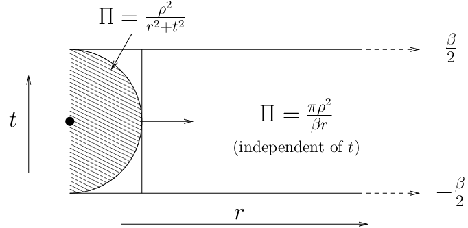
where we exploit the respective spherical symmetry of the ’t Hooft potentials. In both regions we only have to deal with rational functions which can be easily integrated exactly. Apart from this extra complication the strategy is the same as in the zero temperature case and is illustrated in Fig. 8. The results are given in appendix A.2.1 and B.2.1.

The main objective for small separations is to capture adequately the singularity structure, for which it is sufficient to restrict ourselves to the $T=0$ region. To capture contributions that do not blow up, we add the large separation contributions truncated at the pair separation $(R_{t},R_{s})$. The results are given in appendix A.2.2 and B.2.2. Apart from considering different functional forms for the ’t Hooft potential this is the same procedure as for the $T=0$ asymptotic interactions and is illustrated in Fig. 9.

As in the $T=0$ case, the quark overlaps in the small separation region are qualitatively incorrect. However, this region is again dominated by the gluonic repulsion. The latter is not as well approximated as in the $T=0$ case but the agreement is still on the $10\%$ level and, most importantly, qualitatively correct, see Fig. 10. In contrast, the large separation asymptotic formulas work well.

The IILM is defined by its partition function,

with $S_{\mathrm{int}}$ defined in (15) and the single instanton density given by $d(\rho)=d_{0}(\rho)d_{T}(\rho)$. The zero temperature contribution $d_{0}$ is given in [44]. The finite temperature term describes the screening in the plasma of coherent field excitations exceeding the inverse temperature scale $\beta$, and is given by [12] [34],

Apart from book-keeping related technicalities, the major challenge is to adequately simulate instanton–anti-instanton molecules, the structures responsible for the chiral symmetry restoration within the IILM [15], [16], [35]. Detailed numerical studies at finite temperature have been performed in [34]. For the mass parameters used in these latter simulations no technical problems were encountered. However, for the small quark masses that we determined in the $T=0$ simulations, we found that standard Monte Carlo techniques faced severe problems with the strong attraction between instanton–anti-instanton pairs. In [45] we have argued that this technical problem will occur quite generally for the semi-classical expansion with small quark masses. In that paper we have set up the framework to deal with these algorithmic issues by adapting techniques from chemical engineering and computational chemistry and developed for the study of strongly associating fluids.

The instanton–anti-instanton pair interactions become ever stronger and more localised for small quark masses, and random sampling methods will generically miss these configurations. We therefore need to preferentially sample the attraction centres. This can be achieved by resorting to biased Monte Carlo schemes. They exploit the large redundancy in devising transition probabilities $P_{ij}$ that satisfy detailed balance,

where the equilibrium distribution $P^{\mathrm{eq}}$ is given by the partition function. Specifically, the degeneracy follows from the fact that the transition probability consists of two parts, the proposal probability, $\mathcal{P}_{ij}$, and the acceptance probability, $\mathcal{A}_{ij}$,

To satisfy (22), the acceptance probability is given by

which is the Metropolis prescription.

Recently, efficient and general purpose algorithms have been developed to achieve this importance sampling; we will use [48], the Unbonding–Bonding algorithm (UB). This algorithm focuses not on the union of all the interaction regions, a complicated and case-specific geometrical problem, but on the individual interaction regions and all the possible routes that lead to the same final state.

For the IILM, we choose the bonding region to consist of the two disconnected valleys of strong interaction, see Fig. 11, and take them to be hypercubes for simplicity. The precise size of the box is a free parameter and will be chosen to achieve the fastest convergence. We will check that the results do not depend on the bonding box parameters, within statistical uncertainties. We will now present the transition probabilities for the different types of updates; details can be found in [45].

The forward and backward transition probabilities for the UB moves of instanton $i$ are given by

with $\delta^{B}_{i}=1$ if $i$ is bonded and $\delta^{B}_{i}=0$ otherwise. We denote by $N^{B}_{I}$ ($N^{B}_{A}$) the number of bonded instantons (anti-instantons) and $N^{B}_{I}(i)$ is the number of anti-instantons that instanton $i$ is bonded to, and analogously for $N^{B}_{B}(i)$. Unprimed quantities are evaluated before the move whereas primed ones denote the same quantity after the move. The individual bonding and unbonding transition probabilities are given by

The bonding move consists of choosing uniformly an instanton and an anti-instanton, and to place the instanton $i$ uniformly in the bonding region $V_{j}$ of the anti-instanton $j$. The unbonding move consists of choosing uniformly one of the bonded instantons and to place it uniformly in the simulation box.

Insertion and deletion will be constructed along the lines of the UB algorithm by either placing the instanton $i$ into the bonding region of an anti-instanton or removing the bonded instanton $i$. Adding up all possible paths, including the unbiased one, we get

Here $p_{b}$ is the a-priori-probability to perform biased moves.

It has also been argued that cluster moves are important to achieve good mixing of the Markov chain [28]. We assume that $I-A$ pairs are the dominant clusters that form. The pair displacements consist of translating the pair as a whole or to displace one of the constituents within the bonding region of its partner, and the resulting transition probabilities are obvious. The pair insertions and deletions are given by

where $N_{P}$ is the number of pairs. The last terms in each line follow from randomly and independently inserting/deleting an instanton and an anti-instanton. We found that inclusion of these unbiased moves enhances the acceptance rates at high temperature when we approach the dilute gas limit.

So far we have only discussed the spatial arrangements of the instantons. However, the interaction also depends on the colour degrees of freedom [10]. This further technicality can be dealt with by adapting techniques for orientation dependent forces in molecular dynamics simulations. To this end we define the measure in colour space by the Boltzmann factor of the pair interaction. This ensures that $U$ is chosen so as to increase the interaction. More precisely, given the position of the instanton within the bonding box of its partner anti-instanton, we want to sample the following equilibrium distribution:

where $dU_{I}$ is the Haar measure over $SU(3)$. Note that we neglect the influence of the neighbouring instantons and anti-instantons; we could include them but since the fermionic interaction involves a determinant the computation would become rather costly.

We cannot sample this distribution analytically, but we can sample it exactly within a Monte Carlo scheme [10]. Using the fact that the Haar measure is invariant under group composition and also that the interactions (4) and (14) depend on $U=U^{\dagger}_{I}U_{A}$, it is natural to work with $U$. To sample (34), we choose a set of $N$ different colour matrices uniformly over $SU(3)$, i.e. according to the Haar measure. We select one among those $N$ matrices according to the probability

with $S^{\mathrm{pair}}_{i}=S^{\mathrm{pair}}_{\mathrm{int}}(U_{i},x_{I},x_{A})$. Now, remember that the transition probability is given by a proposal and acceptance probability, and that the former includes any a-priori-probabilities for generating the proposed state. Thus, the orientational bias includes the generation probability of the set of matrices, and is given by

The selection probability and the first $N$ volume factors are obvious. The additional $N-1$ volume factors need further explanation. Given the form (24) for the acceptance probability, apart from the $N$ matrices used in (35), we need to generate another $N-1$ trial matrices that combine with the matrix selected in the forward move to form the set of $N$ matrices necessary to evaluate the orientational bias, (35), in the backward move. Finally, the extra enhancement of $N$ is necessary because we are not so much interested in $U_{i}$ being generated at the $i\mathrm{th}$ trial but rather that the value $U_{i}$ is selected. Thus we must marginalise over the label $i$: adding up all the permutations of the set of trial matrices modulo the permutations of the subset of the $N-1$ matrices that are not selected produces the extra $N$ factor. Of the $2N-1$ volume factors $2N-2$ will cancel in general²² 2 One might think that all $2N-1$ volume factors drop out, but in general we might add new moves that select $U$ with a rule different from (35); in such a case we only need $2N-2$ trial matrices. and so we can simplify (36) to

which we recognise as an approximation to (34); note, however, that within the MC scheme is exact, i.e. the results do not suffer from any discretisation errors. Including the orientation bias amounts to multiplying the bonding box volume factors $V_{j}$ by (37).

We found that the interaction are rather self-similar when expressed in units of $\bar{\rho}=\sqrt{\rho_{I}^{2}+\rho^{2}_{A}}$. Thus, the bonding region depends on both particles that make up the pair through a function of their sizes. We choose the functional form of the size dependence to be given by

By construction, $V_{\mathrm{UB}}$ is independent of the specific pair, and we will tune it to achieve fast convergence.

The IILM does not lead to confinement; from a heuristic point of view this follows from the simple fact that the Harrington–Shepard calorons have a vanishing Polyakov loop, the order parameter of the phase transition. It has been in argued in [37] that at low temperatures the instanton density should only depend very weakly on temperature and that, in particular, the result (21) is only applicable in the plasma, i.e. deconfined, phase. In the hadronic phase the fundamental degrees of freedom are not screened and the heat bath consists mainly of pions. We will follow the prescription put forward in [34] and include in (21) a phenomenological term that mimics the transition from the confined to the deconfined phase. We have decided to investigate this with the following two choices, see Fig. 12:

The functional form $d^{1}_{T}$ for the transition between hadronic and plasma phase has been used in [34]. The functional form $d^{2}_{T}$ is chosen on the basis that, intuitively, it should lead to a more symmetrical behaviour around $T_{*}$. With these two choices we will get a rough idea on the systematics due to these phenomenological terms. We’ve introduced two new parameters into the IILM; they will be fixed by comparing our results to available lattice data.

So far these modified screening factors are purely phenomenological. However, the more general non-trivial holonomy calorons [23, 25, 24] [26], that might play a crucial role in driving the confinement/deconfinement phase transition, have been shown to lead to mean instanton sizes that depend very weakly on temperature in the confined phase [11]. Given the assumptions of that paper, the change of the Polyakov loop with temperature is responsible for the different screening behaviour of instantons in the confined and deconfined phase: in the former, the equilibrium state corresponds to an ensemble of maximally non-trivial holonomy calorons which are not screened, whereas the latter consists of trivial holonomy Harrington–Shepard calorons which are strongly screened. We can therefore interpret the modified screening factors (39) as an effective description of the change of the Polyakov loop as the system evolves through the phase transition. Generalising the IILM to include these calorons in the future, we might be able to describe the plasma screening effects self-consistently.

Note that for low temperatures the IILM should not be very different from the $T=0$ case, which was well dealt with by ordinary Monte Carlo. We can use this regime to test the more advanced Monte Carlo scheme against unbiased simulations. In Fig. 13 we plot the thermalisation history at such low temperatures for two different set of quark masses; the latter are given by the physical masses determined in [44] and the second set has the same dimensionless strange quark mass and identical light quarks with a value of ten times the physical up quark. We can clearly see that the histories for the biased and unbiased simulations are very similar.

As the temperature is increased, ordinary Monte Carlo fails for the set of physical quark masses. For intermediate temperatures, around $T_{*}$, there is a substantial difference in the results from biased and unbiased simulations. Even for the set of larger masses there are differences visible to the naked eye, see Fig. 14. For these temperatures instanton–anti-instanton pair formation, the mechanism that drives the chiral symmetry restoration in the IILM, is supposed to be very important. We find that the number of pairs is indeed quite different with $\langle N_{P}\rangle\approx 20$ for biased and $\langle N_{P}\rangle\approx 7$ for unbiased simulations and physical quarks. For the larger quark masses we find that the difference in the number of pairs between biased, $\langle N_{P}\rangle\approx 16$, and unbiased, $\langle N_{P}\rangle\approx 11$, simulations is less pronounced, as expected.

At temperatures well inside the plasma phase, ordinary Monte Carlo fails completely to describe the system accurately for physical quark masses, see Fig. 15. In this case the number of pairs is very different, $\langle N^{\mathrm{biased}}_{P}\rangle\approx 18$ and $\langle N^{\mathrm{unbiased}}_{P}\rangle\approx 1$. Note, however, that the number of pairs has decreased for the higher temperatures.

Simulations at larger masses converge (slowly) to the correct equilibrium distribution. Actually, ordinary Monte Carlo perform better at high temperature than around $T_{*}$ for these larger quark masses. The reason is that the ensemble equilibrates in a very dilute state, so that there are only a few instanton–anti-instanton pairs, $\langle N^{\mathrm{biased}}_{P}\rangle\approx 4.5$ and $\langle N^{\mathrm{unbiased}}_{P}\rangle\approx 1.5$. Note, again, that the pair concentration has dropped with respect to temperatures around $T_{*}$. It turns out that, quite generally, the molecule concentration drops with increasing temperature, because the energy-dominated pair configurations have a smaller and smaller entropy and are outweighed by the entropy-dominated configurations; the latter correspond to a truly random ensemble of instantons at a high enough temperature. This will happen for physical quark masses as well, albeit at higher temperatures.

To be a bit more precise, consider the contribution to the partition function of an instanton–anti-instanton pair, which we approximate by its dilute gas limit and by the contribution from the bonding box. The latter dominates, and hence biased simulations might be needed, if

The contribution from the two instanton measures have cancelled on both sides, and we used $V=N/2\int d$ for the dilute gas. The overbar is meant to indicate the average over the bonding box, size and colour orientations.

Using the 1-loop formula for the instanton measure and choosing one specific size with $T\rho=\mathrm{const}$, this leads to

We only display explicitly the temperature dependence for the one-loop instanton measure (first term), the gluonic interaction (second term), the quark interaction (third term) and the scaling with temperature of the bonding box (fourth term). It turns out that the gluonic contribution is bounded by $5$ for $N_{f}=3$. Hence the $\log T$ term is negative and the dilute gas approximation becomes better and better as the temperature increases, see also Fig. 16. For higher temperatures, when more quark flavours become active, the trend seems to be reversed. Note, however, that this conclusion completely neglects the high-frequency quantum interaction, which should be investigated in the future to study this issue further.

The UB algorithm is only useful if the results do not depend strongly on the precise implementation, i.e. the actual definition of the bonding box. We checked this by using different bonding boxes for three different temperatures, i.e. above, around and below $T_{*}$, see Table 1. We found that the results agree very well for temperatures below $T_{*}$. This corroborates our expectations that biased Monte Carlo is not essential in that regime. For a modest sample of $200$ independent configurations³³ 3 This relates to $\langle N\rangle$; the autocorrelation time for $\langle Q^{2}\rangle$ was always smaller, effectively leading to a larger sample size. The better agreement on the latter quantity corroborates the expectation that the differences among bonding boxes vanish for infinite sample size., we also find rather good agreement for the higher temperatures where random sampling fails. We have also checked the dependence on the a-priori-probabilities⁴⁴ 4 The data in Table 1 corresponds to one particular choice for the a-priori-probabilities.; we find again that the results only depend weakly on these choices for the small sample size we have used. Autocorrelation times, however, depend much more strongly on the bonding box; this allows us to fine-tune the parameters to achieve efficient sampling. The bonding box $B_{4}$ will be used for the final simulation.

We argued that for sufficiently high temperatures, the IILM goes over to a dilute ensemble. It turns out that for high dilution the numerical manipulation of the quark overlaps becomes unstable because the overlap matrix becomes nearly degenerate. To render the evaluation of the fermionic interaction stable we need to decompose the overlap matrix into smaller non-degenerate blocks.

To achieve this, we truncate the interactions to zero above a certain cutoff; it is a function of the pair sizes and determines which instantons interact with each other. Given this cutoff, we can built clusters of pairwise interacting instantons. The overlap matrix $T_{IA}$ is then decomposed into a direct sum according to these clusters. Not only does this render the numerical manipulations stable, but it also leads to a dramatic speed increase. Incidentally, we also use a cutoff for the gluonic interactions to get a better scaling with the number of instantons.

The topological susceptibility approaches the dilute gas approximation for temperatures above approximately $250\,\mathrm{MeV}$, and, like the quark condensate, does not seem to be sensitive to the high concentration of instanton–anti-instanton molecules, see Fig. 23.

Guided by the ideas of [16] that the IILM leads to a mixture of a highly correlated and a random component, it is natural to identify the unbonded instantons as the dominant contribution to the topological susceptibility; the molecules, at least at zeroth order, do not lead to charge fluctuations and thus cannot account for the topological susceptibility. For a random ensemble $N_{r}$ it follows that

We found, however, that the population of unbonded instantons is far too large to be responsible for the small topological susceptibility, under the assumption that $N_{ub}$ is a completely random ensemble, see Fig. 24. Again, as in the case of the quark condensate, it is the non-interacting instantons, not the unbonded instantons, that fit the bill. Note that for higher temperatures, $T\approx 600\,\mathrm{MeV}$, where the pair concentration is still quite high, the concentration of unbonded and non-interacting instantons becomes equal and there is no more distinction between the two. For lower temperatures a coupling between unbonded and bonded instantons still exists.

Note that, in the chiral limit, the topological susceptibility is related to the quark condensate through chiral perturbation theory. It is therefore consistent that the condensate and the topological susceptibility behave rather similarly.

Finally, it is worth noting that the topological susceptibility, and also the quark condensate, are not overly sensitive to the free parameters $T_{*}$ and $\Delta T$, see Fig. 25.

In order to solve the strong CP problem, Peccei and Quinn introduced a new field into the Standard Model of particle physics [32, 31]. It was soon realised that this field gives rise to a new light particle, a pseudo-Goldstone boson, the axion [49, 46]. At the time it seemed natural to tie the axion to the electro-weak scale but laboratory experiments have ruled out such an axion. Leaving the scale of the PQ field $f_{a}$ free, and large to evade the previously mentioned constraints, the so-called ‘invisible’ axions were born, e.g. [8, 50, 21, 36].

Through their weak couplings to ordinary matter, invisible axions can play the role of a dark matter candidate. They have a rich phenomenology, and can be produced through a variety of production channels: the thermal scenario (similar to WIMP production), cosmic string decay (axions are the the Goldstone boson of a spontaneously broken $U_{\mathrm{PQ}}(1)$ symmetry) and the so-called misalignment mechanism. The latter is essentially the PQ mechanism: due to the anomalous $U_{\mathrm{PQ}}(1)$ symmetry an axion mass term is generated through the coupling of the axion to the topological charge

This term combines with the vacuum angle $\theta$ and the axion field can be shifted to get rid of $\theta$, i.e. the vacuum angle becomes a dynamical field, the axion angle $\theta_{a}$. This is the key insight because now we can evoke the principle of least action to argue that $\theta_{a}\to 0$ dynamically to solve the strong CP problem.

Indeed, integrating out the gluons, we can determine the axion mass from the effective action,

according to

References

• [1] B. Allés, M. D’Elia, and A. Di Giacomo. Topological susceptibility at zero and finite T in SU(3) Yang-Mills theory. Nucl. Phys. B, 494:281–292, 1997.
• [2] Y. Aoki, S. Borsanyi, S. Durr, Z. Fodor, S. Katz, S. Krieg, and K. Szabo. The QCD transition temperature: results with physical masses in the continuum limit II. JHEP, 06:088, 2009.
• [3] Y. Aoki, Z. Fodor, S.D. Katz, and K.K. Szabo. The QCD transition temperature: results with physical masses in the continuum limit. Phys.Lett. B, 643:46–54, 2006.
• [4] K. Bae, J. Huh, and J. Kim. Update of axion CDM energy. JCAP, 0809:005, 2008.
• [5] A. A. Belavin, A. M. Polyakov, A. S. Schwartz, and Yu. S. Tyupkin. Pseudoparticle solutions of the Yang-Mills equations. Phys. Lett. B, 59:85–87, 1975.
• [6] M. Chu and S. Schramm. Instanton content of finite temperature QCD matter. Phys. Rev. D, 51:4580–4586, 1995.
• [7] C. Detar and R. Gupta. Toward a precise determination of Tc with 2+1 flavors of quarks. PoS, LAT2007:179, 2007.
• [8] M. Dine, W. Fischler, and M. Srednicki. A simple solution to the strong CP problem with a harmless axion. Phys. Lett. B, 104:199, 1981.
• [9] D.I. Dyakonov and V.Yu. Petrov. Instanton-based vacuum from the Feynman variational principle. Nucl. Phys. B, 245:259–292, 1984.
• [10] D. Frenkel and B. Smit. Understanding Molecular Simulation. Academic Press, 2002.
• [11] P. Gerhold, E.M. Ilgenfritz, and M. Müller-Preussker. An S​U​(2)SU(2) KvBLL caloron gas model and confinement. Nucl. Phys. B, 760:1–37, 2007.
• [12] D.J. Gross, R.D. Pisarski, and L.G. Yaffe. QCD and instantons at finite temperature. Rev. Mod. Phys., 53:43–80, 1981.
• [13] B. Grossman. Zero energy solutions if the Dirac equation in an N-pseudoparticle field. Phys. Lett. A, 61:86–88, 1977.
• [14] B.J. Harrington and H.K. Shepard. Periodic Euclidean solutions and the finite-temperature Yang-Mills gas. Phys. Rev. D, 17:2122–2125, 1978.
• [15] E. Ilgenfritz and E. Shuryak. Chiral symmetry restoration at finite temperature in the instanton liquid. Nucl. Phys. B, 319:511–520, 1989.
• [16] E. Ilgenfritz and E. Shuryak. Quark-induced correlations between instantons drive the chiral phase transition. Phys. Lett. B, 325:263–266, 1994.
• [17] E.M. Ilgenfritz, M. Müller-Preussker, and D. Peschka. Calorons in S​U​(3)SU(3) lattice gauge theory. Phys.Rev. D, 71:116003, 2005.
• [18] J. I. Kapusta. Finite-temperature field theory. CUP, 1993.
• [19] F. Karsch. Recent lattice results on finite temperature and density QCD, part II. PoS, LAT2007:015, 2007.
• [20] F. Karsch and E. Laermann. Susceptibilities, the specific heat and a cumulant in two flavor QCD. Phys. Rev. D, 50:6954, 1994. Private communication with Frithjof Karsch.
• [21] J. Kim. Weak-interaction singlet and strong CP invariance. Phys. Rev. Lett., 43:103, 1979.
• [22] E.W. Kolb and M.S. Turner. The Early Universe. Westview Press, 1990.
• [23] T.C. Kraan and P. van Baal. Exact TT-duality between Calorons and Taub-NUT spaces. Phys.Lett. B, 428:268–276, 1998.
• [24] T.C. Kraan and P. van Baal. Monopole Constituents inside S​U​(N)SU(N) Calorons. Phys.Lett. B, 435:389–395, 1998.
• [25] T.C. Kraan and P. van Baal. Periodic Instantons with non-trivial Holonomy. Nucl.Phys. B, 533:627–659, 1998.
• [26] K. Lee and C. Lu. S​U​(2)SU(2) Calorons and Magnetic Monopoles. Phys.Rev. D, 58:025011, 1998.
• [27] A. Linde. Inflation and Axion Cosmology. Phys. Lett., B201:437, 1988.
• [28] G. Orkoulas and A.Z. Panagiotopoulos. Free energy an dphase equilibria for the restricted primitive model of ionic fluids from Monte Carlo simulations. J. Chem. Phys., 101:1452–1459, 1994.
• [29] B. Ovrut and H. Schnitzer. The Decoupling Theorem and Minimal Subtraction. Phys. Lett. B, 100:403–406, 1981.
• [30] B. Ovrut and H. Schnitzer. Effective Field Theory in Background Gauge. Phys. Lett. B, 110:139–142, 1982.
• [31] R. Peccei and H. Quinn. Constraints imposed by CP conservation in the presence of pseudoparticles. Phys. Rev. D, 16:1791, 1977.
• [32] R. Peccei and H. Quinn. CP conservation in the presence of pseudoparticles. Phys. Rev. Lett., 38:1440, 1977.
• [33] G. Rodrigo and A. Santamaria. QCD matching conditions at thresholds. Phys. Lett. B, 313:441–446, 1993.
• [34] T. Schäfer and E.V. Shuryak. Interacting instanton liquid in QCD at zero and finite temperatures. Phys.Rev. D, 53:65226542, 1996.
• [35] T. Schäfer, E.V. Shuryak, and J.J.M. Verbaarschot. Chiral phase transition and instanton-anti-instanton molecules. Phys. Rev. D, 51:1267–1281, 1995.
• [36] M. Shifman, A. Vainshtein, and V. Zakharov. Can confinement ensure natural CP invariance of strong interactions? Nucl. Phys. B, 166:493, 1980.
• [37] E. Shuryak and M. Velkovsky. Instanton density at finite temperatures. Phys. Rev. D, 50:3323–3327, 1994.
• [38] E.V. Shuryak. Toward the quantitative theory of the instanton liquid (II). The S​U​(2)SU(2) gluodynamics. Nucl. Phys. B, 302:574–598, 1988.
• [39] E.V. Shuryak and J.J.M. Verbaarschot. QCD Instantons at finite temperature. Nucl. Phys. B, 364:255–282, 1991.
• [40] Max Tegmark, Anthony Aguirre, Martin Rees, and Frank Wilczek. Dimensionless constants, cosmology and other dark matters. Phys. Rev., D73:023505, 2006.
• [41] M. Turner. Cosmic and local mass density of invisible axions. Phys. Rev. D, 33:889, 1986.
• [42] M. Turner and F. Wilczek. Inflationary Axion Cosmology. Phys. Rev. Lett., 66:5–8, 1991.
• [43] C. Vafa and E. Witten. Parity conservation in quantum Chromodynamics. Phys. Rev. Lett., 53:535, 1984.
• [44] O. Wantz. The topological susceptibility from grand canonical simulations in the interacting instanton liquid model: zero temperature calibrations and numerical framework. Nucl. Phys. B, 829:48–90, 2010.
• [45] Olivier Wantz. The topological susceptibility from grand canonical simulations in the interacting instanton liquid model: strongly associating fluids and biased Monte Carlo. Nucl. Phys. B, 829:91–109, 2010.
• [46] S. Weinberg. A new light boson? Phys. Rev. Lett., 40:223, 1978.
• [47] S. Weinberg. Effective Gauge Theories. Phys. Lett. B, 91:51–55, 1980.
• [48] S. Wierzchowski and S.A. Kofke. A general-purpose biasing scheme for Monte Carlo simulation of associating fluids. J. Chem. Phys., 114:8752–8762, 2001.
• [49] F. Wilczek. Problem of strong PP and TT invariance in the presence of Instantons. Phys. Rev. Lett., 40:279, 1978.
• [50] A. Zhitnitsky. On Possible Suppression of the Axion Hadron Interactions. (In Russian). Sov. J. Nucl. Phys., 31:260, 1980.