On the Stability of Periodic Solutions of the Generalized Benjamin-Bona-Mahony Equation
Abstract
We study the stability of a four parameter family of spatially periodic traveling wave solutions of the generalized Benjamin-Bona-Mahony equation to two classes of perturbations: periodic perturbations with the same periodic structure as the underlying wave, and long-wavelength localized perturbations. In particular, we derive necessary conditions for spectral instability to perturbations to both classes of perturbations by deriving appropriate asymptotic expansions of the periodic Evans function, and we outline a nonlinear stability theory to periodic perturbations based on variational methods which effectively extends our periodic spectral stability results.
1 Introduction
In this paper, we consider the generalized Benjamin-Bona-Mahony (gBBM) equation
| (1) |
where , , and is a prescribed nonlinearity. In particular, we will be most interested in the case of a power-law nonlinearity as this is when our results are most explicit. Notice that when , (1) is precisely the Benjamin-Bona-Mahony equation (BBM), or the regularized long-wave equation, which arises as an alternative model to the well known Korteweg-de Vries equation (KdV)
as a description of gravity water waves in the long-wave regime (see [4, 19]). In applications, various other nonlinearities arise which facilitates our consideration of the generalized BBM equation. For suitable nonlinearities, equation (1) admits traveling wave solutions of the form with wave speed which are are either periodic or asymptotically constant. Solutions which are asymptotically constant are known as the solitary waves, and they correspond to either homoclinic or heteroclinic orbits of the traveling wave ODE
| (2) |
obtained from substituting the traveling wave ansatz into (1). The stability of such solutions to localized, i.e. , perturbations is well known [5, 18, 20]: the solitary waves form a one parameter family of traveling wave solutions of the gBBM which can be indexed by the wave speed . A given solitary wave solution of the is nonlinearly (orbitally) stable if the so called momentum functional
is an increasing function at , i.e. if , and is exponentially unstable if is negative. In the special case of a power-nonlinearity , it follows that such waves are nonlinearly stable if , while for there exists a critical wavespeed such that the waves are nonlinearly unstable for and stable for .
In [18], Pego and Weinstein found the mechanism for the instability of the solitary waves to be as follows: linearizing the traveling gBBM equation
| (3) |
about a given solitary wave solution of (2) and taking the Laplace transform in time yields a spectral problem of the form considered on the real Hilbert space . The authors then make a detailed analysis of the Evans function , which plays the role of a transmission coefficient familiar from quantum scattering theory: in particular, measures intersections of the unstable manifold as and the stable manifold as of the traveling wave ODE. As a result, if Re and , it follows that the spectral problem has a non-trivial solution, and hence belongs to the point spectrum of the linearized operator11 1 By a standard argument, the essential spectrum can be shown to lie on the imaginary axis, and hence any spectral instability must come from the discrete spectrum.. Using this machinery, Pego and Weinstein were able to prove that as and
for and some constant . Thus, if is decreasing at , then by continuity there must exist a real such that , which proves exponential instability of the underlying traveling wave.
The focus of the present work concerns the stability properties of spatially periodic traveling wave solutions of (1) and in contrast to its solitary wave counterpart, relatively little is known in this context. Most results in the periodic case falls into one of the following two categories: spectral stability with respect to localized or bounded perturbations [6, 8, 16, 15], and nonlinear (orbital) stability with respect to periodic perturbations[1, 2, 9, 11, 17]. The spectral stability results rely on a detailed analysis of the spectrum of the linearized operator in a given Hilbert space representing the class of admissible perturbations: in our case, we will consider both , corresponding to localized perturbations, and , corresponding to -periodic perturbations where is the period of the underlying wave. Notice that unstable spectrum in represents a high-frequency instability and hence manifests itself in the short time instability (local well-posedness) of the underlying solution, while unstable spectrum near the origin corresponds to instability to long wavelength (low-frequency) perturbations, or slow modulations, and hence manifests itself in the long time instability (global well-posedness) of the underlying solution. Notice that on a mathematical level, the origin in the spectral plane is distinguished by the fact that the traveling wave ordinary differential equation (2) is completely integrable. Thus, the tangent space to the manifold of periodic traveling wave solutions can be explicitly computed, and the null space of the linearized operator can be built up out of a basis for this tangent space.
Our analysis of the linearized spectral problem on parallels that of the solitary wave theory described above, in that we compare the large real behavior of the corresponding periodic Evans function to the local behavior near the origin, thus deriving a sufficient condition for instability. The stability analysis to arbitrary localized perturbations is more delicate and follows the general modulational theory techniques of Bronski and Johnson [8]: unlike the solitary wave case, the spectrum of the linearized operator about a periodic wave has purely continuous spectrum and hence any spectral instability must come from the essential spectrum. As a result, there are relatively few results in this case. In the well known work of Gardner [12], it is shown that periodic traveling wave solutions of (1) of sufficiently long wavelength are exponentially unstable whenever the limiting homoclinic orbit (solitary wave) is unstable. The mechanism behind this instability is the existence of a “loop” of spectrum in the neighborhood of any unstable eigenvalue of the limiting solitary wave. More recently, Hǎrǎguş carried out a detailed spectral stability analysis in the case of power-nonlinearity for waves sufficiently close to the constant state determining when the spectrum of the linearized operator is confined to the imaginary axis. We, on the other hand, consider arbitrary periodic traveling waves with essentially arbitrary nonlinearity: as a result of this level of generality we are unable to make conclusive spectral stability statements but instead can only determine -spectral stability near the origin: this is determined by an asymptotic analysis of the periodic Evans function near the origin resulting in a modulational instability index which determines the local normal form of the spectrum. However, we find that this analysis yields quite a bit of information about the spectrum of the underlying wave.
The orbital stability results rely on the now familiar energy functional techniques or Grillakis, Shatah, and Strauss [13] used in the study of solitary type solutions. This program has recently been carried out by Johnson [17] in the case of periodic traveling waves of the generalized Korteweg-de Vries equation. The corresponding theory for the gBBM equation is nearly identical to the analysis in [17], and hence will only be outlined in this work.
Finally, we study the behavior of the above indices in a long-wavelength limit in the case of a power-nonlinearity . For such non-linearities, we gain an additional scaling in the wave speed which allows explicit calculations of the leading order terms in this stability index. A naive guess would be that the value of the orientation index would converge to the solitary wave stability index. This is not the case, however, since the convergence of long-wavelength periodic waves to solitary waves is non-uniform, implying such a limit is highly singular. What is true is that the sign of the finite-wavelength instability index converges to the sign of the solitary wave stability index. Since this index was derived from an orientation index calculation, only its sign matters and thus we show that this stability index is in some sense the correct generalization of the stability index used in the study of solitary waves of (1). Moreover, the sign of the modulational stability index converges to the same sign as the solitary wave index, implying that periodic waves of (1) in a neighborhood of a solitary wave are modulationally unstable if and only if the nearby solitary wave unstable. Notice this does not follow directly from the work of Gardner described above: there it is proved that there exists a “loop” of spectrum in the neighborhood of the origin which is the it continuous image of a circle, but to our knowledge it has never been proved that this map is injective.
The outline for this paper is as follows. In section 2 we review the basic properties of the periodic traveling wave solutions of (1), and in section 3 we review the basic properties of the periodic Evans function utilized throughout this work. In section 4, we begin our analysis by considering stability of the -periodic traveling wave to -periodic perturbations. In particular, we first determine the orientation index, which provides sufficient information for spectral instability to such perturbations, and then discuss how this index plays into the nonlinear stability theory. In section 5, we conduct our modulational instability analysis. In section 6 we analyze the results of sections 4 and 5 in a solitary wave limit, thus extending the well known results of Garnder. Finally, we close in section 7 with a brief discussion and closing remarks.
2 Properties of the Periodic Traveling Waves
In this section, we describe the basic properties of the periodic traveling waves of the gBBM equation (1). For each , a traveling wave is a solution of the traveling wave ODE (2), i.e. they are stationary solutions of (1) in a moving coordinate frame defined by . Clearly (2) defines a Hamiltonian ODE and can be reduced to quadrature: in particular, the traveling waves satisfy the relations
| (4) |
where and are real constants of integration and with . Notice that the solitary waves correspond to and fixed by the asymptotic values of the solution. However, the parameters and are free parameters: we must only require that the effective potential
have a non-degenerate local minimum (see Figure 1). Note that this places restrictions on the allowable parameter regime for our problem: we will always assume we are in the interior of this region, and that the roots of the equation are simple and such that for . In particular, this guarantees the classical “turning points” are functions of the parameters , , and . Thus, the periodic solutions of (2) form a four parameter family of solutions while the solitary waves form a codimension two subset. Notice however that the translation invariance, corresponding to the parameter is not essential to our theory and can be modded out. Hence, we consider the periodic traveling wave solutions of (1) as a three parameter family of the form . The partial differential equation (1) has, in general, the three conserved quantities
| (5) | |||||
which correspond to the mass, momentum, and Hamiltonian (energy) of the solution, respectively. These three quantities are considered as functions of the traveling wave parameters , , and and their gradients with respect to these parameters will play an important role in the foregoing analysis. It is important to notice that when restricted to the four-parameter family of periodic traveling wave solutions of (1), the mass can be represented as . Since all our results concern this four-parameter family, we will always work with this simplified expression for the mass functional.


As is standard, one can use equation (4) to express the period of the periodic wave as
The above interval can be regularized at the square root branch points by the a standard procedure (see [8] for example) and hence represents a function of . Similarly, the mass and momentum can be expressed as
and can be regularized as above. In particular, it follows that one can differentiate these functionals restricted to the periodic wave with respect to the parameters . The gradients of these quantities will play an important role in the subsequent theory.
It is useful to notice the following connection to the classical mechanics corresponding to the traveling wave ODE. The classical action in the sense of action angle variables is given by
| (6) |
While is not itself conserved, it does provide a useful generating function for the conserved quantities of (1). Indeed, it is clear the classical action satisfies the relation
where , which immediately establishes several useful identities between the gradients of , , and . For example, it follows that and .
Finally, we make a few notes on notation. Throughout the forthcoming analysis, various Jacobians of maps from the traveling wave parameters to the period and conserved quantities of the gBBM flow will become important. We adopt the following Possion bracket style notation
for the Jacobian determinants with the analogous notation for larger determinants
Notice that the nonvanishing of such quantities encodes geometric information about the underlying manifold of periodic traveling wave solutions of (1): more will be said on this in the coming sections.
3 The Periodic Evans Function
We now begin our stability analysis of a -periodic traveling wave by considering a solution to the partial differential equation (1), i.e. a stationary solution of (3), of the form
where is considered as a small perturbation parameter. Substituting this into (1) and collecting terms at yields the linearized equation where , , and . Since this linearized equation is autonomous in time, we may seek separated solutions of the form , which yields the spectral problem
| (7) |
Throughout this paper, we consider the above operators as acting on corresponding to spatially localized perturbations, or on corresponding to -periodic perturbations. In both cases, the operator is a positive operator and is hence invertible and hence (7) can be written as a spectral problem for a linear operator:
As has is a differential operator with periodic coefficients, the natural setting to study the spectrum of the operator is that of Floquet theory. We begin with the following standard definition.
Definition 1.
The monodromy operator is defined to be the period map
where satisfies the first order system
| (8) |
subject to the initial condition , where is the identity matrix and
It now follows from an easy calculation that (7) has no point spectrum in . Indeed, suppose is a vector solution of (8) corresponding to a non-trivial eigenfunction of with eigenvalue . From the definition of the monodromy operator, we have
for any . It follows that can be at most bounded on and must not decay as . This observation leads one to the following definition.
Definition 2.
We say if there exists a non-trivial bounded function such that or, equivalently, if there exists a such that
Following Gardner [12] we define the periodic Evans function to be
Finally, we say the periodic solution is spectrally stable if does not intersect the open right half plane.
Remark 1.
First, notice by the Hamiltonian nature of (7), is symmetric with respect to reflections about the real and imaginary axis. Thus, spectral stability occurs if and only if .
Secondly, since we are interested primarily with the roots of for on the unit circle, we will frequently work with the function for , which is actually the function considered by Gardner.
It follows that we can parameterize the continuous spectrum of the operator by the Floquet parameter :
In particular, the zero’s of the function for a fixed correspond to the -eigenvalues of the operator resulting from the map applied to (7), and hence the continuous spectrum of can be parameterized by a one-parameter family of eigenvalue problems. By a standard result of Gardner, if , then the multiplicity of as a periodic eigenvalue of the corresponding linear operator is precisely the multiplicity of as a root of the Evans function. As we will see below, the integrable structure of (2) implies that the function has a zero of multiplicity (generically) three at . For small then, there will be in general three branches of roots of which bifurcate from the origin. Assuming these branches are analytic22 2 In general, for each , the theory of branching solutions of non-linear equations guarantees the existence of a natural number such that is an analytic function of . As we will see in our case, the Hamiltonian nature of the linearized operator assures that , and hence the roots are in fact analytic functions of the Floquet parameter. in , it follows that a necessary condition for spectral stability is thus
| (9) |
This naturally leads to the use of perturbation methods in the study of the spectrum of near the origin, i.e. modulational instability analysis of the underlying traveling wave. As we will see, the first order terms of a Taylor series expansion of the three branches can be encoded as roots of a cubic polynomial, and hence spectral stability is determined by the sign of the associated discriminant. Moreover, it follows by the Hamiltonian structure of (7) that in fact if (9) holds and the roots of the cubic polynomial are distinct.
We conclude this section by reviewing some basic global features of the spectrum of the linearized operator which are useful in a local analysis near . We also state some important properties of the Evans function which are vital to the foregoing analysis.
Proposition 1.
The -spectrum of the operator has the following properties:
- (i)
There are no isolated points of the spectrum. In particular, the spectrum generically consists of piecewise smooth arcs.
- (ii)
The entire imaginary axis is contained in the spectrum, i.e.
Moreover, the Evans function satisfies the following:
- (iii)
.
- (iv)
with
Proof.
The first claim, that the spectrum is never discrete, follows from a basic lemma in the theory of several complex variables: namely that, if for fixed the function has a zero of order at and is holomorphic in a polydisc about then there is some smaller polydisc about so that for every in a disc about the function (with fixed) has roots in the disc . For details see the text of Gunning[14]. It is clear from the implicit function theorem that is a smooth function of as long as where represents the standard cofactor matrix.
Claim follows from Abel’s formula and the fact that , where is as in (8).
Next, we prove claim . Since is invariant under the transformation and , we have . If we define as above and such that
it follows that
Therefore, as claimed.
Claim now follows from a symmetry argument. Since is real on the real axis, it follows by Schwarz reflection that for we have . For then the Evans function takes the form
It follows that
so that the roots of for a fixed are symmetric about the unit circle. Since there must be three such roots, one must live on the unit circle and hence as claimed. ∎
4 Periodic Instabilities: Spectral and Nonlinear Stability Results
In this section, we make a detailed analysis of the stability of a given periodic traveling wave solution of (1) to perturbations with the same periodic structure: such perturbations correspond to in the above theory. We begin by a spectral stability analysis, and then conclude with a brief discussion of a nonlinear (orbital) stability result.
4.1 Periodic Spectral Instabilities
Let be a -periodic traveling wave solution of (1). Considering the spectral stability of such a solution of perturbations which are -periodic is equivalent to studying the spectrum of the linear operator on the real Hilbert space . We begin with the following lemma.
Lemma 1.
Let be the solution of the traveling wave equation (2) satisfying and . A basis of solutions to the first order system
is given by
Moreover, a particular solution to the inhomogeneous problem
where is given by
Proof.
This is easily verified by differentiating (2) with respect and the parameters , , and . ∎
By the above lemma, three linearly independent solutions of the differential equation
are given by the functions , , and above. Notice that here we are considering the formal operators with out any reference to boundary conditions. In order to understand the structure of the periodic null-space of the operator , we now use Lemma 1 to express the solution matrix in this basis at and .
Notice by hypothesis, for any the solution satisfies
| (10) | |||||
| (11) | |||||
| (12) |
and, moreover, it follows from (2) that . Defining where , , are vector functions corresponding to the solutions , , and , respectively, it follows by differentiating the above relations that
| (13) |
Differentiating the relation with respect to gives
and hence these solutions are linearly independent at , and hence for all . Moreover, using the chain rule to differentiate (10)-(12), we see the matrix is given by
It follows that is a rank one matrix.
Our immediate goal is to relate this information to the structure of the periodic Evans function . As we will see, the fact that is rank one allows for significant simplifications in the perturbation calculations. Without this fact, one would have to compute variations in the vector solutions at to an extra degree, which would force the use of multiple applications of variation of parameters along the same null direction. In particular, we have the following lemma.
Lemma 2.
For , the periodic Evans function satisfies
Proof.
Let , , be three linearly independent solutions of (8), and let be the solution matrix with columns . Expanding the above solutions in powers of as
and substituting them into (8), the leading order equation becomes
Using Proposition 1, we choose .The higher order terms in the above expansion yield
| (14) |
where and denotes the first component of the vector . Notice that for each of the higher order terms , we require . Notice this implies that in a neighborhood of , where is defined in (13). The solution of the inhomogeneous problem is given by the variation of parameters formula
for . Notice we have used the identities and extensively in the above formula, which can be easily derived via equation (4). Indeed, differentiating (4) with respect to and subtracting immediately yields the first identity.
Now, notice that it would be a daunting task to use (4.1) to the specified order needed. However, the integrable structure of (7) allows for an alternative, yet equivalent, expression in the case which makes a seemingly second order calculation come in at first order. Indeed, in this case equation (14) is equivalent to and hence it follows from Proposition 1 that we can choose
where the above constants in front of and are determined by the requirement . Thus, one can determine the second order variation of in by using (4.1) to compute the first order variation of the function defined above. Defining , it follows that can be expanded as
where and the higher order terms are determined by (4.1). Thus,
and in particular a straightforward calculation yields
The proof is complete by recalling that . ∎
Remark 2.
Notice that the formula for differs from that derived by Bronski and Johnson [8] in the case of the generalized KdV by a factor of one-half, which comes from that fact the differences in the definitions of the momentum functionals in each work: in particular, the factor of in (5) is not present in [8].
Assuming the Jacobian is non-zero, it follows that zero is a -periodic eigenvalue of of multiplicity three. By computing the orientation index
it is clear that we will have exponential periodic instability of the underlying wave if this index is negative. With this in mind, we now compute the large behavior of the periodic Evans function in the next lemma.
Lemma 3.
The function satisfies the following asymptotic relation:
Proof.
This follows from a simple calculation. By introducing variable change in (7), it follows that as the monodromy operator satisfies the asymptotic relation
| (18) |
where
The eigenvalues of are rather complicated, but for large and real they satisfy , where
It follows that
and thus, since , the leading order term of
as comes from , which completes the proof. ∎
We are now able to state our first main theorem for this section.
Theorem 1.
let be a periodic solution of (2). If is negative at , then the number of roots of (i.e. the number of periodic eigenvalues of ) on the positive real axis is odd. In particular, if the period is an increasing function of energy at , i.e. , then the periodic traveling wave is spectrally unstable to -periodic perturbations if and only if is negative at .
Proof.
By our work in the proof of Lemma 2, we know that . Thus, if for small positive , the number is negative for small positive . Since is positive for real sufficiently large, we know that for some . Moreover, since it follows that has either one or two negative -periodic eigenvalues. Since the number of negative eigenvalues of provide an upper bound for the number of unstable -periodic eigenvalues of with positive real part (see Theorem 3.1 of [18]), and since implies has precisely one negative -periodic eigenvalue (see Lemma 4.1 of [17]) the proof is now complete. ∎
We now wish to give insight into the meaning of at the level of the linearized operator . To this end, we consider the linearized operator as acting on , the space of -periodic functions on . To begin, we make the assumption that and do not simultaneously vanish. This assumption will be shown equivalent with the periodic null-space reflecting the Jordan structure of the monodromy at the origin. Throughout this brief discussion, we assume that : trivial modifications are needed if vanishes but does not. First, define the functions
Clearly, each of these functions belong to and
In particular, we have used the fact that on . Thus, it follows that the periodic null space of is generated spanned by the functions and . Moreover, since
the assumption that and do not simultaneously vanish implies that , thus reflecting the Jordan normal form of the period map at .
Finally, we study the structure of the generalized periodic null space, and seek conditions for which there is no non-trivial Jordan chain of length two. By the Fredholm alternative, such a chain exists if and only if
Thus, the vanishing of is equivalent with a change in the generalized periodic-null space of the linearized operator . This insight has a nice relationship with formal Whitham modulation theory. One of the big ideas in Whitham theory is to locally parameterize the periodic traveling wave solution by the constants of motion for the PDE evolution. The non-vanishing of certain Jacobians is precisely what allows one to do this. In fact, the non-vanishing of is equivalent to demanding that, locally, the map have a unique inverse: In other words, the constants of motion for the gBBM flow are good local coordinates for the three-dimensional manifold of periodic traveling wave solutions (up to translation). Similarly, non-vanishing of and is equivalent to demanding that the matrix
have full rank, which is equivalent to demanding that the map (for fixed ) have a unique inverse, i.e. two of the conserved quantities provide a smooth parametrization of the family of periodic traveling waves of fixed wave-speed.
To summarize, the vanishing of , is connected with a change in the Jordan structure of the linearized operator considered on . In particular, ensures the existence of a non-vanishing Jordan piece in the generalized periodic null-space of dimension exactly one. Moreover, and perhaps more importantly, it guarantees that infinitesimal variations in the constants arising from reducing the family of periodic traveling waves to quadrature are enough to generate the entire generalized periodic null-space of the linearized operator : such a condition is obviously not necessary in our calculations, but provides significant simplifications in the theory.
4.2 Nonlinear Periodic-Stability
We now compliment Theorem 1 by considering in what sense the Jacobian affects the nonlinear stability of a periodic traveling wave solution of (1) to -periodic perturbations. Clearly, the positivity of this index is necessary for such stability but it is not clear if this is also necessary. Indeed, the analysis presented below allows for the possibility that a periodic traveling wave which is spectrally stable to -periodic perturbations could be nonlinearly unstable to such perturbations: such a result would stand in stark contrast to the solitary wave theory where these two notions of stability are equivalent (assuming the nondegeneracy condition ). More will be said on this at the end of this section.
Such analysis has recently been carried out in the context of the generalized Korteweg-de Vries equation by Johnson [17]. There, sufficient conditions for nonlinear stability to -periodic perturbations were derived in terms of Jacobians of various maps between the parameter space and the period, mass, and momentum. As the theory for the gBBM equation is nearly identical to this work, we only review the main points of the analysis here and refer the reader to [17] for details.
To begin, we assume the nonlinearity is such that the Cauchy problem for (1) is globally well posed on a real Hilbert space of -periodic functions defined on , which we equip with the standard inner product. In particular, we require to be a subspace of . Also, we identify the dual space through the usual pairing. Now, we fix a periodic traveling wave solution of (1) and notice that we can write the linearized spectral problem (7) about in the form
where is an augmented energy functional defined by
where , , and are the energy, momentum, and energy functionals defined on defined by
In particular, notice that each of these functionals are left invariant under spatial translations and hence it is appropriate to study the stability of periodic solutions of (2) up to translation. To this end, we introduce a semi-distance defined via
and we seek conditions for which the following statement is true: If is near as measured by the semidistance , then the solution of (1) with initial data stays close to a translate of for all time.
We begin by noticing that is a critical point of the augmented energy functional . In order to determine the nature of this critical point, it is necessary to analyze the second derivative of . If is positive definite, then nonlinear stability follows by standard arguments. However, one sees after an easy calculation that
which is clearly not positive definite by the translation invariance of (1). Indeed, since and is not monotone it follows by standard Sturm-Liouville arguments that zero is either the second or third eigenvalue of with respect to the natural ordering on . By Lemma 4.1 of [MJ1], we it follows that considered on has precisely one negative eigenvalue, a simple eigenvalue at zero, and the rest of the spectrum is positive and bounded away from zero if . If , then either the the null space or the number or negative eigenvalues jumps by one: a situation which can seemingly not be handled by the present variational analysis33 3 However, see the recent work of Bronski, Johnson, and Kapitula [BrJK]..
Thus, assuming it follows that is a degenerate critical point of with one unstable direction and one neutral direction. In order to get rid of the unstable direction, simply notice that the evolution of (1) does not occur on the entire space , but on the codimension two subset
Clearly is a smooth submanifold of containing all translates of the function . Defining to be the tangent space of at , i.e.
we have by Lemma 4.3 of [MJ1] that the quadratic form induced by is positive definite on if and
| (19) |
where is defined as above. Since the underlying periodic wave is spectrally unstable if by Theorem 1, the only interesting case in which (19) holds is when and are positive. With these conditions in mind, it follows that the augmented energy is coercive on near with respect to the semi-distance , from which nonlinear stability follows: see Proposition 4.2 and the corresponding proof in [17] for details. Summarizing, we have the following orbital stability result.
Theorem 2.
By Theorem 2, it follows that may not be sufficient for nonlinear stability of a periodic traveling wave of (1). In particular, notice that in the solitary wave theory it is always true that the operator has only one eigenvalue, and hence it is always true that any unstable eigenvalues of the linearized operator must be real. In the periodic context, however, we see this is only true if , which is not true for all periodic traveling wave solutions of (1): for example, it is clear that the cnoidal wave solutions of the modified BBM equation corresponding to (1) with of sufficiently long wave period satisfy . Thus, it may be possible in certain situations that the linearized operator has unstable -periodic eigenvalues which are not real. Moreover, even if and are positive, and hence one has periodic spectral stability, it is not clear from this analysis whether one has nonlinear stability since the sign of the Jacobian still plays a seemingly large role44 4 However, one should be aware of the recent works [11] and [9] in which perturbation methods and more delicate functional analysis were used to analyze this problem for the gKdV in a way which provides more precise results than the above variational methods.. This phenomenon, which stands in contrast to the solitary wave theory, is a reflection of how the periodic traveling wave solutions of (1) have a much richer structure than the solitary waves, allowing for possibly more interesting dynamics.
5 Modulational Instability Analysis
In this section, we begin our study of the spectral stability of periodic traveling wave solutions of the gBBM equation (1) to arbitrary localized perturbations. In particular, our methods will detect instabilities of such solutions to long wavelength perturbations, i.e. to slow modulations of the underlying wave. Such stability analysis seems to be a bit more physical than the periodic stability analysis conducted in the previous section in the following sense: in physical applications, one should probably never expect to find an exact spatially periodic wave. Instead, what one often sees is a solution which on small space-time scales seems to exhibit periodic behavior, but over larger scales is clearly seen not to be periodic due to a slow variations in the amplitude, frequency, etc, i.e. one sees slow modulations physical parameters defining the solution. Thus, it seems natural to study the stability of such solutions by idealizing them as exact spatially periodic waves and then study the stability of this idealized wave to slow modulations in the underlying parameters. This is precisely the goal of the modulational stability analysis in this paper. Moreover, in terms of the long-time stability of such solutions it is clear that a low frequency analysis of the linearized operator is vital to obtaining suitable bounds on the corresponding solution operator of the nonlinear equation.
To begin, notice that by Lemma 2 the linearized operator has a -periodic eigenvalue at the origin in the spectral plane of multiplicity (generically) three. Thus, as we allow small variations in the Floquet parameter, we expect that there will be three branches of continuous spectrum which bifurcate from the origin. According to Proposition 1, one of these branches must be confined to the imaginary axis, and hence will not contribute to any spectral instability. In order to determine if the other two branches bifurcate off the imaginary axis or not, we derive an asymptotic expansion of the function for . As a result, we will see that, to leading order, the local structure of the spectrum near the origin is governed by a homogeneous polynomial of degree three in the variables and . We then evaluate the coefficients of the resulting polynomial in terms of Jacobians of various maps from the parameters to the quantities , , and . To this end, we begin with the following Lemma.
Lemma 4.
If , the equation has the following normal form in a neighborhood of :
| (20) |
whose Newton diagram is depicted in Figure 2.

Proof.
Define functions and on a neighborhood of by
| (21) |
where is small. In particular, notice that
Now, using the fact that the spectral problem (7) is invariant under the transformation , it follows that the matrices and are similar for all . In particular, it follows that
By comparing the and terms above to those in (21), we have the relations
Differentiating with respect to and evaluating at immediately implies and . Similarly, it follows that . The proof is now complete by Lemma 2 and the fact that . ∎
It follows that the structure of in a neighborhood of the origin is, to leading order, determined by the above homogeneous polynomial in and . Due to the triple root of at the implicit function theorem fails, but can be trivially corrected by considering the appropriate change of variables. This leads us to the following theorem giving a modulational stability index for traveling wave solutions of (1).
Theorem 3.
With the above notation, define
and suppose that . If , then the spectrum of the linearized operator in a neighborhood of the origin consists of the imaginary axis with a triple covering. If , then in a neighborhood of the origin consists of the imaginary axis with multiplicity one together with two curves which are tangent to lines through the origin.
Proof.
Since, to leading order in and , the Evans function is homogeneous by Lemma 4 it seems natural to work with the projective coordinate . Making such a change of variables, Lemma 4 implies the equation can be written as
| (22) |
where is continuous in a neighborhood of the origin. Let denote the three roots of the above cubic in corresponding to . Assuming it follows that are distinct and hence the implicit function theorem applies giving three distinct solutions of (22) in a neighborhood of each of the . In terms of the original variable , this gives three solution branches
If , then , giving three branches of spectrum emerging from the origin tangent to the imaginary axis. From the Hamiltonian symmetry of (7), the spectrum is symmetric with respect to reflections across the imaginary axis and hence implies these thee branches of spectrum must in fact lie on the imaginary axis, proving the existence of an interval of spectrum of multiplicity three on the imaginary axis. In the case , it follows that one of the roots, say, is real while the other two occur in a complex conjugate pairs, giving one branch along the imaginary axis and two branches emerging from the origin tangent to lines through the origin with angel : see Figure 3. ∎
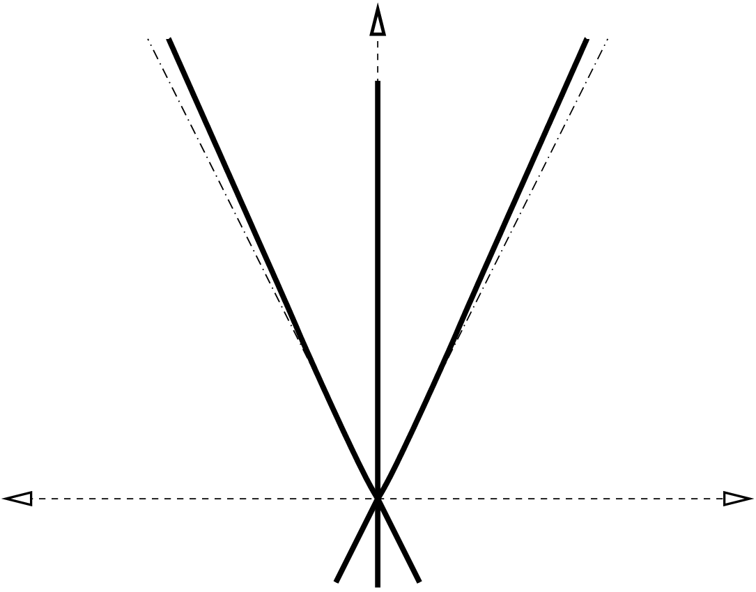
Remark 3.
The modulational instability index derived above is considerably more complicated than the one derived by Bronski and Johnson [8] for generalized Korteweg-de Vries equation
| (23) |
When considering the spectral stability of periodic traveling wave solutions of (23), it was shown that there exists a modulational instability index such that implies modulational instability, and implies modulational stability. In this case, the dominant balance is somewhat simpler due to the fact that the trace of the operator vanishes, and hence the term in the corresponding Newton diagram vanishes. As a result, the modulational instability index took the form
where here represents the Evans function for equation (23). It follows that the sign of does not effect the modulational instability of such periodic solutions of equation (23). However, in the case of the gBBM equation, the fact that seems to suggest that the sign of the sign of this orientation index (see next section) has an impact on the modulational stability of the periodic traveling wave. In fact, in section 4 we prove exactly this fact in the case of a power-nonlinearity : we prove the long-wavelegth periodic traveling wave solutions of (1) are modulationally unstable if and only if the limiting homoclinic orbit (solitary wave) is exponentially unstable.
Our next goal is to use the integrable nature of (2) to express in terms of the underlying periodic traveling wave . This is the content of the following lemma.
Lemma 5.
We have the following identity:
Proof.
This proof is essentially an extension of that of Lemma 2. Using the same notation, a straightforward yet tedious calculation yields
The proof is completed by noting that since and .∎
Thus, the modulational stability of a given periodic traveling wave solution to (1) can be determined from information about the underlying solution itself. Interestingly, from Lemma 5 the modulational instability index seems to depend directly on the turning point , a feature not seen in the corresponding analysis of the generalized KdV equation in [8]. However, one can trace this dependence back to the definition of in Lemma 2 and hence seems to be unavoidable. In the next section, we will analyze the above stability indices in neighborhoods of homoclinic orbits in phase space, complimenting the results of Gardner [12] by providing stability results in this limit.
6 Analysis of Stability Indices in the Solitary Wave Limit
The goal of this section is to study the long wavelength asymptotics of the stability indices derived in the previous sectios. Throughout, we restrict ourselves to the case of a power-nonlinearity : this restriction is vital to our calculation since in this case we gain an additional scaling symmetry. In particular, if satisfies the differential equation
| (24) |
then a straight forward calculation shows that we can express the periodic solution as
| (25) |
This additional scaling allows explicit calculations of , which ends up determining the stability of periodic traveling wave solutions of (1) of sufficiently long wavelength.
A reasonable guess would be that long-wavelength periodic traveling wave solutions of (1) have the same stability properties as the limiting homoclinic orbit (solitary wave). However, as noted in the introduction, this is a highly singular limit and so it is not immediately clear whether such results are true. It is well known that the solitary wave is spectrally unstable if and only if and for some critical wave speed . It follows from the work of Gardner [12] that periodic waves below the homoclinic orbit in phase space which are sufficiently close to the homoclinic orbit are unstable if the solitary wave is unstable. In particular, it is proved that the linearized operator for the periodic traveling wave with sufficiently long wavelength has a “loop” of spectrum in the neighborhood of any unstable eigenvalues of the limiting solitary wave. Thus, Gardner’s analysis deduces instability of long wavelength periodic waves from instability of the limiting solitary waves. The results of this section compliment this theory by also proving that the stability of the limiting wave is inherited by nearby periodic waves below the homoclinic orbit in phase space.
In terms of the finite-wavelength instability index, it seems reasonable by Theorem 1 to expect that for periodic traveling wave solutions below the seperatrix of sufficiently long wavelength, for if and only if and . What is unclear is whether such a result should be true for the modulational instability index . Indeed, although Gardner’s results prove that the spectrum of the linearization about a periodic traveling wave of sufficiently long wavelength in the neighborhood of the origin contains the image of a continuous map of the unit circle, to our knowledge it has never been proved that this map is injective. Thus, it is not clear from Gardner’s results whether a modulational instability will arise from this eigenvalue since it is possible this “loop” is confined to the imaginary axis: we show that in fact one has modulational instability in this limit precisely when the limiting solitary wave is unstable.
The main result for this section is the following theorem, which is based on asymptotic estimates of the instability indices derived in section 3. In particular, we prove the sign of both instability indices in the solitary wave limit is determined by the sign of , where is the momentum of the periodic wave . The proof is based on a more technical lemma, which shows that for waves of sufficiently long wavelength, i.e. for sufficiently close to zero. We begin by outlining the proof of the following theorem, and then fill in the necessary lemma’s afterward.
Theorem 4.
Let for some and let , with sufficiently small, be a periodic solution of the traveling wave ODE (2) which corresponds to an orbit below the homoclinic orbit in phase space. If is sufficiently large, then is modulationally and nonlinearly stable for all . For , there exists a critical wave speed such that if is sufficiently large, the solution is orbitally and modulationally stable if , while it is modulationally unstable for .
Proof.
Without loss of generality, suppose that the periodic solution of (2) corresponds to a branch cut of the function with positive right end point. Now, when and are small there are two turning points in the neighborhood of the origin and a third turning point which is bounded away from the origin. In the solitary wave limit a straight forward calculation gives that From this, it follows that the period satisfies the asymptotic relation
| (26) |
To see this, notice that by our assumptions on , , and we can write where is positive on the set . The period can then be expressed as
The integral over the set is clearly as . For the other integral, notice that
on the set . Thus, in the limit as we have
from which (26) follows. Similar computations yield the following asymptotic relations for and sufficiently small:
Thanks to the above scaling we know can be expressed as a linear combination of , , and . Similarly, can be expressed as a linear combination of , and . It follows that the asymptotically largest minor of for and small is and, moreover,
In Lemma 6 below, we will show that for such and . Moreover, it is clear that for such periodic waves with sufficiently long wavelength satisfy . Therefore, it follows that both stability indices are determined by the sign of in the solitary wave limit. The theorem now follows by Lemma 7 below. ∎
Remark 4.
Notice that the fact that the finite wavelength instability index is determined by the sign of in the solitary wave limit is not surprising, since this is exactly what detects the stability of the limiting solitary waves. What is surprising is that the same quantity controls the modulational stability index in the same limit. As mentioned above, it has not been know if the instability of the limiting solitary wave forces a modulational instability: the answer is shown to be affirmative by Theorem 4.
In order to complete the proof Theorem 4, we must prove a few more technical lemmas. The first is used in showing that the sign of the modulational and finite-wavelength instability indices are determined completely by the sign of in the limit as tend to zero. This is the result of the following lemma.
Lemma 6.
For sufficiently small, for all .
Proof.
Notice it is sufficient to prove for all and sufficiently small. Now, can be written as
where is the smallest positive root of the polynomial equation . Setting , we have
where is the smallest positive root of the polynomial . Notice for a fixed wave speed , is a smooth function of for sufficiently small and satisfies
The goal is to now rewrite the above integral over a fixed domain and show that the integrand is a decreasing function of for a fixed .
Making the substitution yields the expression
Now, we can use the above expansion of to conclude that
is positive on the open interval for all and , which completes the proof. ∎
Finally, it is left to analyze the asymptotic behavior for a fixed wavespeed of the quantity in the solitary wave limit. This is the content of the following lemma.
Lemma 7.
In the case of power non-linearity , we the momentum satisfies
in the solitary wave limit , where . In particular, for and sufficiently small, if then for all while if then for and for , where
Proof.
The proof is based on scaling and a limiting argument, as well as a modification of the analysis in [18]. To begin, let satisfy the differential equation (24) so that can be expressed via scaling as in (25), and assume with out loss of generality that be an absolute max of . Clearly, the solitary wave limit corresponds to taking with fixed wave speed . Notice that on any compact subset of , we have
uniformly as on for some . Using (24), it follows that
where are the roots of satisfying the original hypothesis of the roots of . Since as , the dominated convergence theorem along with the fact that is a function of and implies that
Similarly, it follows that
Using (25), we now have
as , and hence it follows by differentiation that
as claimed, where we have used that . The lemma now follows by solving the quadratic equation for and recalling the restriction that . ∎
The proof of Theorem 4 is now complete by Lemmas 6 and 7. As a consequence, the finite-wavelength instability index seems to be a somewhat natural generalization of the solitary wave stability index, in the sense that the well known stability properties of solitary waves are recovered in a long-wavelength limit. Moreover, this gives an extension of the results of Gardner in the case of generalized BBM equation by proving the marginally stable eigenvalue of the solitary wave at the origin contributes to modulational instabilities of nearby periodic waves when ever the solitary wave is unstable.
Finally, we wish to make an interesting comment concerning the elliptic function solutions of the modified BBM (mBBM) equation with . In the special case in our theory of , it turns out that all periodic traveling wave solutions can be expressed in terms of Jacobi elliptic functions: when such solutions correspond to cnoidal waves, expressible in terms of the function, while when such solutions correspond to dnoidal waves, expressible in terms of the function . By Theorem 4, it follows that the dnoidal waves with sufficiently small(corresponding to ) are always modulationally stable and nonlinearly (orbitally) stable to perturbations with the same periodic structure. What is unclear from our above analysis is whether the cnoidal waves with sufficiently close to (corresponding to ) are exhibit a sense of stability: such waves correspond to periodic orbits outside the seperatrix in phase space, and hence Theorem 4 does not apply to such solutions. Moreover, such waves do not approach any particular solitary wave in any uniform way, even on compact subsets, and hence it is not clear if the stability of the limiting solitary waves at all influences the cnoidal waves. However, notice that for sufficiently close to unity one must have and hence by the analysis in the proof of Theorem 4 we have . Therefore, the cnoidal waves of the mBBM with sufficiently long wavelength are modulationally unstable. Similarly, in this solitary wave limit one has
and hence one has spectral instability to periodic perturbations if for sufficiently small. Using the complex analytic calculations of Bronski, Johnson, and Kapitula [9], we can solve the corresponding Picard-Fuchs system and see that
| (27) |
See the appendix for more details of this calculation. Since for such solutions, we find that . Thus, the cnoidal wave solutions of the mBBM equation of sufficiently large wavelength are exponentially unstable to perturbations with the same periodic structure. In particular, it seems like the index serves as Maslov index in this problem: when it is which signals the stability near the solitary wave, while it is when55 5 While we have not actually proven this here (we only showed this is the case for cnoidal solutions of mBBM), we suspect this is the case for all nonlinearities of the form for . For examples where this phenomenon is studied in more cases see [9]. . This index arises naturally in the solitary wave setting: see [10] for details and discussion. In particular, notice that in the solitary wave setting of Pego and Weinstein and in the long wavelength analysis of Gardner, the Maslov index always has the same sign: however, as seen here this is not the case when considering the full family of periodic traveling waves of the gBBM.
7 Concluding Remarks
In this paper, we considered the stability of periodic traveling wave solutions of the generalized Benjamin-Bona-Mahony equation with respect to periodic and localized perturbations. Two stability indices were introduced of the full four parameter family of periodic traveling waves. The first, which is given by the Jacobian of the map between the constants of integration of the traveling wave ordinary differential equation and the conserved quantities of the partial differential equation restricted to the class of periodic traveling wave solutions, serves to count (modulo ) the number of periodic eigenvalues along the real axis. This is, in some sense, a natural generalization of the analogous calculation for the solitary wave solutions, and reduces to this is the solitary wave limit. The second index, which arises as the discriminant of a cubic which governs the normal form of the linearized operator in a neighborhood of the origin, can also be expressed in terms of the conserved quantities of the partial differential equation and their derivatives with respect to the constants of integration of the ordinary differential equation. This discriminant detects modulational instabilities of the underlying periodic wave, i.e. bands of spectrum off of the imaginary axis in an arbitrary neighborhood of the origin.
In our calculations, we heavily used the fact that the ordinary differential equation defining the traveling wave solutions of (1) have sufficient first integrals, and as such is doubtlessly related to the multi-symplectic formalism of Bridges [7]. Many of the ideas from this paper were recently used by the author, in collaboration with Jared C. Bronski, in the analogous study of the spectral stability of periodic traveling wave solutions of the generalized Korteweg-de Vries equation [8]. Thus, the general technique of this paper has been successful in two different cases. These successes gives an indication that a rather general modulational stability theory can be developed using these techniques. It would be quite interesting to compare the rigorous results from this paper to the formal modulational stability predictions of Whitham’s modulation theory [21]. Moreover, the techniques in this paper could eventually lead to a rigorous justification of the Whitham modulation equations for such dispersive equations.
It is not known if our techniques can be extended to equations which are deficient in the number of first integrals. An example would be the generalized regularized Boussinesq equation
A straight forward calculation shows that although this equation admits a five parameter family of traveling wave solutions with a four parameter submanifold of periodic solutions. Although one can still build a four dimensional basis of null-space of the corresponding linearized operator, it is not clear whether the resulting stability indices can be directly related back to geometric information concerning the original periodic traveling wave. Such a result would be very interesting, as it would allow the use of such techniques to several more classes of partial differential equations admitting traveling wave solutions.
Acknowledgements: The author would like to thank Jared C. Bronski for his many useful conversations in the early stages of this work. Also, the author gratefully acknowledges support from a National Science Foundation Postdoctoral Fellowship under grant DMS-0902192.
8 Appendix
In this appendix, we outline the general complex analytic methods used to derive the identity in equation (27). To begin, consider (1) with and let be a given periodic traveling wave. To begin, we notice that that in this case , , and can be represented integrals on a Riemann surface corresponding to the classically allowed region for , where . In particular, defining we have the following integral representations:
where is the classical action defined in (6) and the integrals are taken around the classically allowed region corresponding to the periodic orbit . By differentiating the above relations with respect to the traveling wave parameters, we have the following identities:
In particular, we see that each of the above derivatives can be expressed as linear combinations of the classical action , the moment of the solution
and an integral of the form
We now show that in the case of the mBBM equation, we can find a closed system of seven equations for the integrals in terms of the traveling wave parameters and the quantities , , and . To this end, first notice that for any integer one has the identity
Moreover, integration by parts yields the relation
This yields a linear system of seven equations in seven unknowns known as the Picard-Fuchs system:
The matrix which arises in the above linear system is known as the Sylvester matrix of the polynomials and . In commutative algebra, a standard result is that the determinant of the Sylvester matrix of two polynomials and vanishes if and only if they have a common root. If we now restrict ourselves to , it follows that the above matrix is invertible for all periodic traveling wave solutions of the corresponding mBBM equation. In particular, we can solve the above Picard-Fuchs system and use the fact that to see that
as claimed.
References
- [1] J. Angulo Pava. Nonlinear stability of periodic traveling wave solutions to the Schrödinger and the modified Korteweg-de Vries equations. J. Differential Equations, 235(1):1–30, 2007.
- [2] J. Angulo Pava, J. L. Bona, and M. Scialom. Stability of cnoidal waves. Adv. Differential Equations, 11(12):1321–1374, 2006.
- [3] H. Baumgärtel. Analytic Perturbation Theory for Matrices and Operators, volume 15 of Operator theory: Advances and Applications. Birkhäuser, 1985.
- [4] T. B. Benjamin, J. L. Bona, and J. J. Mahony. Model equations for long waves in nonlinear dispersive systems. Philos. Trans. Roy. Soc. London Ser. A, 272(1220):47–78, 1972.
- [5] J. L. Bona and A. Soyeur. On the stability of solitary-waves solutions of model equations for long waves. J. Nonlinear Sci., 4(5):449–470, 1994.
- [6] N. Bottman and B. Deconinck. Kdv cnoidal waves are linearly stable. Submitted, 2009.
- [7] T. J. Bridges. Multi-symplectic structures and wave propagation. Math. Proc. Cambridge Philos. Soc., 121(1):147–190, 1997.
- [8] J. C. Bronski and M. A. Johnson. The modulational instability for a generalized korteweg-de vries equation. 2008. Submitted.
- [9] J. C. Bronski, M. A. Johnson, and T. Kapitula. An index theorem for the stability of periodic traveling waves of kdv type. Preprint.
- [10] F. Chardard, F. Dias, and T. J. Bridges. Computing the maslov index of solitary waves. part 1: Hamiltonian systems on a 4-dimensional phase space. 2008. preprint.
- [11] B. Deconinck and T. Kapitula. On the orbital (in)stability of spatially periodic stationary solutions of generalized korteweg-de vries equations. 2009. Submitted.
- [12] R. A. Gardner. Spectral analysis of long wavelength periodic waves and applications. J. Reine Angew. Math., 491:149–181, 1997.
- [13] M. Grillakis, J. Shatah, and W. Strauss. Stability theory of solitary waves in the presence of symmetry. I,II. J. Funct. Anal., 74(1):160–197,308–348, 1987.
- [14] R. Gunning. Lectures on Complex Analytic Varieties: Finite Analytic Mapping (Mathematical Notes). Princeton Univ Press, 1974.
- [15] M. Hărăguş. Stability of periodic waves for the generalized BBM equation. Rev. Roumaine Math. Pures Appl., 53(5-6):445–463, 2008.
- [16] M. Hǎrǎguş and T. Kapitula. On the spectra of periodic waves for infinite-dimensional Hamiltonian sytems. To appear: Physica D.
- [17] M. A. Johnson. Nonlinear stability of periodic traveling wave solutions of the generalized korteweg-de vries equation. 2009. Submitted.
- [18] R. L. Pego and M. I. Weinstein. Eigenvalues, and instabilities of solitary waves. Philos. Trans. Roy. Soc. London Ser. A, 340(1656):47–94, 1992.
- [19] D. H. Peregrine. Long waves on a beach. J. Fluid Mechanics, 27:815827, 1967.
- [20] M. I. Weinstein. Existence and dynamic stability of solitary wave solutions of equations arising in long wave propagation. Comm. Partial Differential Equations, 12(10):1133–1173, 1987.
- [21] G. B. Whitham. Linear and nonlinear waves. Pure and Applied Mathematics (New York). John Wiley & Sons Inc., New York, 1999. Reprint of the 1974 original, A Wiley-Interscience Publication.