Multiplicative Bias Corrected Nonparametric Smoothers

Let $(X_{1},Y_{1}),\ldots,(X_{n},Y_{n})$ be $n$ independent copies of the pair of random variables $(X,Y)$ with values in ${\mathbb{R}}\times{\mathbb{R}}$. We suppose that the explanatory variable $X$ has probability density $f$ and model the dependence of the univariate response variable $Y$ to the explanatory variable $X$ through the nonparametric regression model

$$Y=m(X)+\varepsilon.$$

(1)

We assume that the regression function $m(\cdot)$ is smooth and that the disturbance $\varepsilon$ is a mean zero random variable with finite variance $\sigma^{2}$ that is independent of the covariate $X$. Consider the linear smoothers for the regression function $m(x)$ which we can write as

$$\hat{m}(x)=\sum_{j=1}^{n}\omega_{j}(x;h)Y_{j},$$

where the weight function $\omega_{j}(x;h)$ depends on a tuning parameter $h$, that we think of as the bandwidth.

If the weight functions are such that $\sum_{j=1}^{n}\omega_{j}(x;h)=1\mbox{ and }\sum_{j=1}^{n}\omega_{j}(x;h)^{2}=(nh)^{-1}\tau^{2},$ and if the disturbances satisfy the Lindberg-Feller condition, then the linear smoother obeys the central limit theorem

$$\sqrt{nh}\left(\hat{m}(x)-\sum_{j=1}^{n}w_{j}(x;h)m(X_{j})\right)\longrightarrow{\mathcal{N}}(0,\tau^{2}).$$

(2)

We can use (2) to construct asymptotic pointwise confidence intervals for the unknown regression function $m(x)$. But unless the limit of the scaled bias

$$b(x)=\lim_{n\longrightarrow\infty}\sqrt{nh}\left(\sum_{j=1}^{n}w_{j}(x;h)m(X_{j})-m(x)\right),$$

which we call the asymptotic bias, is zero, the confidence interval

$$\left[\hat{m}(x)-Z_{1-\alpha/2}\sqrt{nh}\tau,\hat{m}(x)+Z_{1-\alpha/2}\sqrt{nh}\tau\right]$$

will not cover asymptotically the true regression function $m(x)$ at the nominal $1-\alpha$ level. The construction of valid pointwise $1-\alpha$ confidence intervals for regression smoothers is another motivation for developing estimators with zero asymptotic bias.

Here we present a framework for multiplicative bias reduction. Given a pilot smoother

$$\tilde{m}_{n}(x)=\sum_{j=1}^{n}\omega_{j}(x;h_{0})Y_{j},$$

the ratio

$$V_{j}=\frac{Y_{j}}{\tilde{m}_{n}(X_{j})}$$

is a noisy estimate of $m(X_{j})/\tilde{m}_{n}(X_{j})$, the inverse relative estimation error of the smoother $\tilde{m}_{n}$ at each of the observations. Smoothing $V_{j}$ by

$$\widehat{\alpha}_{n}(x)=\sum_{j=1}^{n}\omega_{j}(x;h_{1})V_{j}$$

yields an estimate for the inverse of the relative estimation error which can be used as a multiplicative correction of the pilot smoother. This leads to the (nonlinear) smoother

$$\widehat{m}_{n}(x)=\widehat{\alpha}_{n}(x)\tilde{m}_{n}(x).$$

(3)

The estimator (3) was studied for fixed design by Linton and Nielsen (1994) and further studied by Jones et al. (1995). In both cases, they assumed that the regression function had four continuous derivatives, and show an improvement in the convergence rate of the corrected estimator. Glad (1998a); Glad (1998b) proposed to use a parametrically guided local linear smoother and Nadaraya-Watson smoother by starting with a parametric pilot. She shows that the resulting estimates improve on the local polynomial estimate as soon as the pilot captures some of the features of the regression function.

We make the following assumptions:

1. 1.

   The regression function is bounded and strictly positive, that is, $b\geq m(x)\geq a>0$ for all $x$.

2. 2.

   The regression function is twice continuously differentiable everywhere.

3. 3.

   The density of the covariate is strictly positive on the interior of its support in the sense that $f(x)\geq b({\mathcal{K}})>0$ over every compact ${\mathcal{K}}$ contained in the support of $f$.

4. 4.

   $\varepsilon$ has finite fourth moments and has a symmetric distribution around zero.

5. 5.

   Given a symmetric probability density $K(\cdot)$, consider the weights $\omega_{j}(x;h)$ associated to the local linear smoother. That is, denote by $K_{h}(\cdot)=K(\cdot/h)/h$ the scaled kernel by the bandwidth $h$ and define for $k=0,1,2,3$ the sums

   $$S_{k}(x)\equiv S_{k}(x;h)=\sum_{j=1}^{n}(X_{j}-x)^{k}K_{h}(X_{j}-x).$$

   Then

   $$\omega_{j}(x;h)=\frac{S_{2}(x;h)-(X_{j}-x)S_{1}(x;h)}{S_{2}(x;h)S_{0}(x;h)-S_{1}^{2}(x;h)}\,K_{h}(X_{j}-x).$$

   We set

   $$\omega_{0j}(x)=\omega_{j}(x;h_{0})\quad\mbox{and}\quad\omega_{1j}(x)=\omega_{j}(x;h_{1}).$$

6. 6.

   The bandwidths $h_{0}$ and $h_{1}$ are such that

   $$h_{0}\to 0,\quad h_{1}\to 0,\quad nh_{0}\to\infty,\quad nh_{1}^{3}\to\infty,\quad\frac{h_{1}}{h_{0}}\to 0\quad\textrm{as}\quad n\to\infty.$$

The positivity assumption (assumption 1) on $m(x)$ is classical when we perform a multiplicative bias correction. It allows to avoid that the terms $Y_{j}/\tilde{m}_{n}(X_{j})$ blows up. Of course, the regression function might cross the $x$-axis. For such a situation, Glad (1998a) proposes to shift all response data $Y_{i}$ a distance $a$, so that the new regression function $m(x)+a$ does not any more intersect with the $x$-axis. Such a method can also be performed here. Assumptions 2–4 are standard to obtain rate of convergence for nonparametric estimators. Assumption 5 means that we conduct the theory for the local linear estimate. The results can be generalized to other linear smoothers. Assumption 6 is not restrictive since it is satisfied for a wide range of values of $h_{0}$ and $h_{1}$.

The proof of the main results rests on establishing a stochastic approximation of estimator (3) in which each term can be directly analyzed.

We will need the following Lemma.

We deduce from Proposition 3.1 and Lemma 3.1 the following Theorem.

We deduce from Theorem 3.1 that if the bandwidth $h_{0}$ of the pilot estimator converges to zero much slower than $h_{1}$, then $\widehat{m}_{n}$ has exactly the same asymptotic variance as the local linear smoother of the original data with bandwidth $h_{1}$. However, for finite samples, the two step local linear smoother can have a slightly larger variance depending on the choice of $h_{0}$. For the bias term, a limited Taylor expansion of $\mu_{n}(x)$ leads to the following result.

It is worth pointing out that we only suppose that the regression function is twice continuously differentiable. We do not add smoothness assumptions. For a study of the local linear estimate in the presence of jumps in the derivative, we refer the reader to Desmet and Gijbels (2009). Combining Theorem 3.1 and Theorem 3.2, we conclude that the multiplicative adjustment performs a bias reduction on the pilot estimator without increasing the asymptotic variance. The asymptotic behavior of the bandwidths $h_{0}$ and $h_{1}$ is constrained by assumption 6. However, it is easily seen that this assumption is satisfied for a large set of values of $h_{0}$ and $h_{1}$. For example, the choice $h_{1}=c_{1}n^{-1/5}$ and $h_{0}=c_{0}n^{-\alpha}$ for $0<\alpha<1/5$ leads to

$$\mathbb{E}_{\star}\left(\widehat{m}_{n}(x)|X_{1},\ldots,X_{n}\right)-m(x)=\mathrm{o}_{p}(n^{-2/5})$$

and

$$\mathbb{V}_{\star}(\widehat{m}_{n}(x)|X_{1},\ldots,X_{n})=\mathrm{O}_{p}\left(n^{-4/5}\right).$$

To illustrate numerically the possible reduction in the bias and associate increase of the variance achieved by the multiplicative bias correction, consider estimating the regression function

$$m(x)=5+3|x|^{5/2}+x^{2}+4\cos(10x)$$

at $x=0$ (see Figure 1).

The local linear smoother tends to under-estimate the regression function at their maximum, and hence, this example will provide a good example. Furthermore, because the second derivative of this regression function is continuous but not differentiable at the origin, the results previously obtained by Linton and Nielsen (1994) do not apply.

The data are simulated according to the model

$$Y_{i}=m(X_{i})+\varepsilon_{i},\quad i=1,\ldots,100,$$

where $\varepsilon_{i}$ are independent $\mathcal{N}(0,1)$ variables. We first consider the local linear estimate with a Gaussian kernel function and we study its performances over a grid of bandwidths $\mathcal{H}=[0.005,0.1]$. For the new estimate, the theory recommends to start with an oversmooth pilot estimate. In this regard, we take $h_{0}=0.1$ and study the performance of the multiplicative bias corrected estimate for $h_{1}\in\mathcal{H}_{1}=[0.005,0.12]$. To explore the stability of our two stages estimator with respect to $h_{0}$, we also consider the choice $h_{0}=0.02$. For such a choice, the pilot estimate clearly undersmoothes the regression function.

Bias and variance of each estimate are calculated at $x=0$. To do this, we compute the value of each estimate at $x=0$ for 200 samples $(X_{i},Y_{i}),i=1,\ldots,100$. The same design $X_{i},i=1,\ldots,100$ is used for each sample. It is generated according to a uniform distribution over $[-1,1]$. The bias at point $x=0$ is estimated by subtracting $m(0)$ at the mean value of the estimate at $x=0$ (the mean value is computed over the 200 replications). Similarly we estimate the variance at $x=0$ by the variance of the values of the estimate at this point. Figure 2 presents squared bias, variance and mean square error of each estimate for different values of bandwidths $h$ for the local linear smoother and $h_{1}$ for our estimate.

The first conclusion is that the corrected estimate has smaller bias than the local linear estimate provided the pilot estimate oversmoothes the regression function. Small values of $h_{0}$ clearly undersmooth the regression function, whatever the choice of $h_{1}$. Moreover, it is worth pointing out that our procedure does not significantly increase the variance. Even if Theorem 3.1 and Theorem 3.2 provide asymptotic results, our simulations show that the asymptotic behavior of our estimate emerges already at modest sample size. Finally, due to the bias reduction, we note that our procedure also reduces the optimal mean square error (see Table 1).

We conclude our local study with a comparison between our estimate and the estimate proposed by Glad (1998a). To do this, we compute the multiplicative bias corrected estimate using three parametric starts:

• •

  first the guide is chosen correctly and belong to the true parametric family:

  $$\tilde{m}_{n}^{1}(x)=\hat{\beta}_{0}+\hat{\beta}_{1}|x|^{5/2}+\hat{\beta}_{2}x^{2}+\hat{\beta}_{3}\cos(10x);$$

• •

  second, we consider a linear parametric guide (which is obviously wrong):

  $$\tilde{m}_{n}^{2}(x)=\hat{\beta}_{0}+\hat{\beta}_{1}x;$$

• •

  finally, we use a more reasonable guide, not correct, but that can reflect some a priori idea on the regression function

  $$\tilde{m}_{n}^{3}(x)=\hat{\beta}_{0}+\hat{\beta}_{1}x+\hat{\beta}_{2}x^{2}+\ldots+\hat{\beta}_{8}x^{8}.$$

All the estimates $\hat{\beta}_{j}$ stands for the classical least square estimates.

The multiplicative bias correction is performed on these parametric starts using the local linear estimate. The performance of the resulting estimates is measured over a grid of bandwidths $\mathcal{H}_{2}=[0.005;0.4]$. Bias and variance of each estimate are still estimated at $x=0$. We keep the same setting as above and all the results are averaged over the same 200 replications. We display in Table 2 the optimal MSE calculated over the grid $\mathcal{H}_{2}$.

As expected, we first observe that the performance clearly depends on the choice of the parametric start. Table 1 and table 2 show that (in term of MSE) the estimate studied in this paper is better than the corrected estimated with parametric start $\tilde{m}_{n}^{2}$ and $\tilde{m}_{n}^{3}$. Unsurprisingly, the best performance are obtained with the parametric guide $\tilde{m}_{n}^{1}$ (which belongs to the true model). In practice, when one has no or few a priori information on the target regression function, the method proposed in the present paper is preferable.

This paper does not conduct any theory to select the two bandwidths $h_{0}$ and $h_{1}$ in an optimal way. If automatic procedures are needed, they can be obtained by adjusting traditional automatic selection procedures for the classical nonparametric estimators (see Burr et al. (2010)). In this part, we propose to use leave-one-out cross validation to choose both $h_{0}$ and $h_{1}$. We then compare the performance of the selected estimate with the local polynomial estimate in term of integrated square error.

Hurvich et al. (1998) report a comprehensive numerical study that compares standard smoothing methods on various test functions. Here, we take the same setting to compare the local linear estimate with its multiplicative bias corrected smoother. In each of the examples, we take the Gaussian kernel $K(x)=\exp(-x^{2}/2)/\sqrt{2\pi}$. We use the following regression functions (see Figure 3):

	(1)	$m_{1}(x)=\sin(5\pi x)$
	(2)	$m_{2}(x)=\sin(15\pi x)$
	(3)	$m_{3}(x)=1-48x+218x^{2}-315x^{3}+145x^{4}$
	(4)	$m_{4}(x)=0.3\exp{[-64(x-.25)^{2}]}+0.7\exp{[-256(x-.75)^{2}]}$

and we take a Gaussian error distribution with standard deviation $\sigma_{j}=0.25\|m_{j}\|_{2}$ for $j=1,\ldots,4$.

We use a cross validation device to select both $h_{0}$ and $h_{1}$. This selection procedure involves solving minimization problem that necessitate a search over a finite grid $\mathcal{H}$ of bandwidths $h_{0}$ and $h_{1}$. Formally, given $\mathcal{H}$, we choose $\hat{h}_{0}$ and $\hat{h}_{1}$ such as

$$(\hat{h}_{0},\hat{h}_{1})=\argmin_{(h_{0},h_{1})\in\mathcal{\mbox{$\mathcal{H}$}}\times\mbox{$\mathcal{H}$}}\frac{1}{n}\sum_{i=1}^{n}(Y_{i}-\widehat{m}_{n}^{i}(X_{i}))^{2}.$$

Here $\widehat{m}_{n}^{i}$ stands for the corrected local polynomial estimate after deleted the $i$th observation. To assess the quality of the selected estimate, we compare its performances with the local polynomial estimate for which the bandwidth is again selected by leave-one-out cross validation. The performance of an estimator $\widehat{m}$ is measured by the integrated square error

$$ISE(\widehat{m})=\int_{0}^{1}\left(m(x)-\widehat{m}(x)\right)^{2}\,\textrm{d}x,$$

and to avoid the boundary effects, the design $X_{1},\ldots,X_{n}$ is generated according to a uniform distribution over $[-0.2,1.2]$.

Table 3 presents the median over 100 replications of

• •

  the selected bandwidths;

• •

  the integrated square error;

• •

  the integrated square error of the local linear estimate divided by the integrated square error of the corrected estimate ($R_{ISE}$).

Figure 4 displays the boxplots of the integrated square error for each estimate.

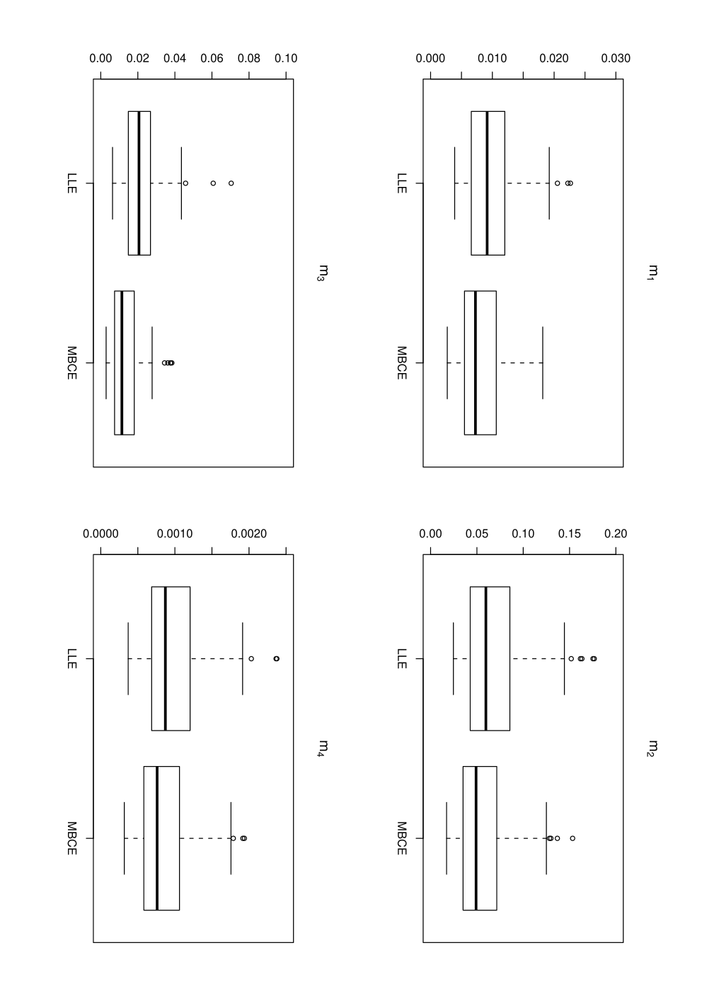
We obtain significant ISE reduction for the four models. As predicted by Theorem 3.1, the data-driven procedure selects $h_{0}$ bigger than $h$: the pilot estimate is oversmoothing the true regression function. Of course, selecting both $h_{0}$ and $h_{1}$ is time consuming and can appear as the price to be paid to improve the local linear smoother.

Figure 5 presents, for the regression function $m_{1}$ with $n=100$ and 100 iterations, different estimators on a grid of points. In lines is the true regression function which is unknown. For every point on a fixed grid, we plot, side by side, the mean over 100 replications of our estimator at that point (left side) and on the right side of that point the mean over 100 replications of the local polynomial estimator. Leave-one-out cross validation is applied to select the bandwidths $h_{0}$ and $h_{1}$ for our estimator and the bandwidth $h$ for the local polynomial estimator. We add also the interquartile interval in order to see the fluctuations of the different estimators.

In this example, our estimator reduces the bias by increasing the peak and decreasing the valleys. Moreover, the interquartile intervals look similar for both estimator, as predicted by the theory.

Write the bias corrected estimator

$$\widehat{m}_{n}(x)=\sum_{j=1}^{n}\omega_{1j}(x)\frac{\tilde{m}_{n}(x)}{\tilde{m}_{n}(X_{j})}Y_{j}=\sum_{j=1}^{n}\omega_{1j}(x)R_{j}(x)Y_{j},$$

and let us approximate the quantity $R_{j}(x)$. Define

$$\bar{m}_{n}(x)=\sum_{j=1}^{n}\omega_{0j}(x)m(X_{j})=\mathbb{E}\left(\tilde{m}_{n}(x)|X_{1},\ldots,X_{n}\right),$$

and observe that

	$\displaystyle R_{j}(x)=$	$\displaystyle\frac{\tilde{m}_{n}(x)}{\tilde{m}_{n}(X_{j})}$
	$\displaystyle=$	$\displaystyle\frac{\bar{m}_{n}(x)}{\bar{m}_{n}(X_{j})}\times\left(1+\frac{\tilde{m}_{n}(x)-\bar{m}_{n}(x)}{\bar{m}_{n}(x)}\right)\times\left(1+\frac{\tilde{m}_{n}(X_{j})-\bar{m}_{n}(X_{j})}{\bar{m}_{n}(X_{j})}\right)^{-1}$
	$\displaystyle=$	$\displaystyle\frac{\bar{m}_{n}(x)}{\bar{m}_{n}(X_{j})}\times[1+\Delta_{n}(x)]\times\frac{1}{1+\Delta_{n}(X_{j})},$

where

$$\Delta_{n}(x)=\frac{\tilde{m}_{n}(x)-\bar{m}_{n}(x)}{\bar{m}_{n}(x)}=\frac{\sum_{l\leq n}\omega_{0l}(x)\varepsilon_{l}}{\sum_{l\leq n}\omega_{0l}(x)m(X_{l})}.$$

Write now $R_{j}(x)$ as

$$R_{j}(x)=\frac{\bar{m}_{n}(x)}{\bar{m}_{n}(X_{j})}\left[1+\Delta_{n}(x)-\Delta_{n}(X_{j})+r_{j}(x,X_{j})\right]$$

where $r_{j}(x,X_{j})$ is a random variable converging to 0 to be define latter on. Given the last expression and model (1), estimator (3) could be written as

	$\displaystyle\widehat{m}_{n}(x)=$	$\displaystyle\sum_{j=1}^{n}\omega_{1j}(x)R_{j}(x)Y_{j}$
	$\displaystyle=$	$\displaystyle\sum_{j=1}^{n}\omega_{1j}(x)\frac{\bar{m}_{n}(x)}{\bar{m}_{n}(X_{j})}m(X_{j})$
		$\displaystyle+\sum_{j=1}^{n}\omega_{1j}(x)\frac{\bar{m}_{n}(x)}{\bar{m}_{n}(X_{j})}\left[\varepsilon_{j}+m(X_{j})\left(\Delta_{n}(x)-\Delta_{n}(X_{j})\right)\right]$
		$\displaystyle+\sum_{j=1}^{n}\omega_{1j}(x)\frac{\bar{m}_{n}(x)}{\bar{m}_{n}(X_{j})}\left(\Delta_{n}(x)-\Delta_{n}(X_{j})\right)\varepsilon_{j}$
		$\displaystyle+\sum_{j=1}^{n}\omega_{1j}(x)\frac{\bar{m}_{n}(x)}{\bar{m}_{n}(X_{j})}r_{j}(x,X_{j})Y_{j}$
	$\displaystyle=$	$\displaystyle\mu_{n}(x)+\sum_{j=1}^{n}\omega_{1j}(x)A_{j}(x)+\sum_{j=1}^{n}\omega_{1j}(x)B_{j}(x)+\sum_{j=1}^{n}\omega_{1j}(x)\xi_{j}.$

which is the first part of the proposition. Under assumption set forth in Section 3.1, the pilot smoother $\tilde{m}_{n}$ converges to the true regression function $m(x)$. Bickel and Rosenblatt (1973) show that this convergence is uniform over compact sets ${\mathcal{K}}$ contained in the support of the density of the covariate $X$. As a result

$$\sup_{x\in{\mathcal{K}}}|\tilde{m}_{n}(x)-\bar{m}_{n}(x)|\leq\frac{1}{2}.$$

So a limited expansion of $(1+u)^{-1}$ yields for $x\in\mathcal{K}$

$$R_{j}(x)=\frac{\bar{m}_{n}(x)}{\bar{m}_{n}(X_{j})}\left[1+\Delta_{n}(x)-\Delta_{n}(X_{j})+\mathrm{O}_{p}\left(|\Delta_{n}(x)\Delta_{n}(X_{j})|+\Delta_{n}^{2}(X_{j})\right)\right],$$

thus

$$\xi_{j}=\mathrm{O}_{p}\left(|\Delta_{n}(x)\Delta_{n}(X_{j})|+\Delta_{n}^{2}(X_{j})\right).$$

Under the stated regularity assumptions, we deduce that

$$\xi_{j}=\mathrm{O}_{p}\left(\frac{1}{nh_{0}}\right).$$

leading to the announced result. Proposition (3.1) is proved.

By definition

$$\limsup_{n\longrightarrow\infty}\mathbb{P}[|\xi_{n}|>ta_{n}]=0$$

for all $t>0$, so that a triangular array argument shows that there exists an increasing sequence $m=m(k)$ such that

$${\mathbb{P}}\left[|\xi_{n}|>\frac{a_{n}}{k}\right]\leq\frac{1}{k}\qquad\mbox{for all }n\geq m(k).$$

For $m(k)\leq n\leq m(k+1)-1$, define

$$\xi^{\star}_{n}=\left\{\begin{array}[]{ll}\xi_{n}&\mbox{ if }|\xi_{n}|<k^{-1}a_{n}\\ 0&\mbox{otherwise.}\end{array}\right.$$

It follows from the construction of $\xi^{\star}_{n}$ that for $n\in(m(k),m(k+1)-1)$,

$${\mathbb{P}}[\xi_{n}\not=\xi_{n}^{*}]={\mathbb{P}}[|\xi_{n}|>k^{-1}a_{n}]\leq\frac{1}{k},$$

which converges to zero as $n$ goes to infinity. Finally set $k(n)=\sup\{k:m(k)\leq n\}$, we obtain

$$\mathbb{E}[|\xi|_{n}^{\star}]\leq\frac{a_{n}}{k(n)}=\mathrm{o}(a_{n}).$$

Recall that

$$\widehat{m}_{n}(x)=\mu_{n}(x)+\sum_{j=1}^{n}\omega_{1j}(x)A_{j}(x)+\sum_{j=1}^{n}\omega_{1j}(x)B_{j}(x)+\mathrm{O}_{P}\left(\frac{1}{nh_{0}}\right).$$

Focus on the conditional bias, we get

	$\displaystyle\mathbb{E}(\mu_{n}(x)|X_{1},\ldots,X_{n})$	$\displaystyle=$	$\displaystyle\mu_{n}(x)$
	$\displaystyle\mathbb{E}(A_{j}(x)|X_{1},\ldots,X_{n})$	$\displaystyle=$	$\displaystyle 0$
	$\displaystyle\mathbb{E}(B_{j}(x)|X_{1},\ldots,X_{n})$	$\displaystyle=$	$\displaystyle\frac{\bar{m}_{n}(x)}{\bar{m}_{n}(X_{j})}\sigma^{2}\Big(\frac{\omega_{0j}(x)}{\bar{m}_{n}(x)}-\frac{\omega_{0j}(X_{j})}{\bar{m}_{n}(X_{j})}\Big).$

Since

$$\sum_{j=1}^{n}\omega_{1j}(x)\omega_{0j}(x)\leq\sqrt{\sum_{j=1}^{n}\omega_{1j}(x)^{2}}\sqrt{\sum_{j=1}^{n}\omega_{0j}(x)^{2}}=\mathrm{O}_{p}\left(\frac{1}{n\sqrt{h_{0}h_{1}}}\right),$$

we deduce that

$$\mathbb{E}\left(\sum_{j=1}^{n}\omega_{1j}(x)B_{j}(x)\Big|X_{1},\ldots,X_{n}\right)=\mathrm{O}_{p}\left(\frac{1}{n\sqrt{h_{0}h_{1}}}\right).$$

This proves the first part of the Theorem.

For the conditional variance, we use the following expansion of the two stages estimator

$$\widehat{m}_{n}(x)=\sum_{j=1}^{n}\omega_{1j}(x)\frac{\bar{m}_{n}(x)}{\bar{m}_{n}(X_{j})}Y_{j}\left(1+\left[\Delta_{n}(x)-\Delta_{n}(X_{j})\right]\right)+\mathrm{O}_{p}\left(\frac{1}{nh_{0}}\right).$$

Using the fact that the residuals have four finite moments and have a symmetric distribution around 0, a moment’s thought shows that

$$\mathbb{V}(Y_{j}\left[\Delta_{n}(x)-\Delta_{n}(X_{j})\right]|X_{1},\ldots,X_{n})=\mathrm{O}_{p}\left(\frac{1}{nh_{0}}\right)$$

and

$$\C(Y_{j},Y_{j}\left[\Delta_{n}(x)-\Delta_{n}(X_{j})\right]|X_{1},\ldots,X_{n})=\mathrm{O}_{p}\left(\frac{1}{nh_{0}}\right).$$

Hence

	$\displaystyle\mathbb{V}_{\star}(\widehat{m}_{n}(x)|X_{1},\ldots,X_{n})$	$\displaystyle=\mathbb{V}\left(\sum_{j=1}^{n}\omega_{1j}(x)\frac{\bar{m}_{n}(x)}{\bar{m}_{n}(X_{j})}Y_{j}\Big|X_{1},\ldots,X_{n}\right)$
		$\displaystyle\hskip 170.71652pt+\mathrm{O}_{p}\left(\frac{1}{nh_{0}}\right).$

Observe that the first term on the right hand side of this equality can be seen as the variance of the two stages estimator with a deterministic pilot estimator. It follows from Glad (1998a) that

$$\mathbb{V}\left(\sum_{j=1}^{n}\omega_{1j}(x)\frac{\bar{m}_{n}(x)}{\bar{m}_{n}(X_{j})}Y_{j}\Big|X_{1},\ldots,X_{n}\right)=\sigma^{2}\sum_{j=1}^{n}\omega_{1j}^{2}(x)+\mathrm{o}_{p}\left(\frac{1}{nh_{1}}\right),$$

which proves the theorem.

Recall that

$$\mu_{n}(x)=\sum_{j\leq n}\omega_{1j}(x)\frac{\bar{m}_{n}(x)}{\bar{m}_{n}(X_{j})}m(X_{j}).$$

We consider the limited Taylor expansion of the ratio

$$\frac{m(X_{j})}{\bar{m}_{n}(X_{j})}=\frac{m(x)}{\bar{m}_{n}(x)}+(X_{j}-x)\left(\frac{m(x)}{\bar{m}_{n}(x)}\right)^{\prime}+\frac{1}{2}(X_{j}-x)^{2}\left(\frac{m(x)}{\bar{m}_{n}(x)}\right)^{\prime\prime}(1+\mathrm{o}_{p}(1)),$$

then

	$\displaystyle\mu_{n}(x)$	$\displaystyle=$	$\displaystyle\bar{m}_{n}(x)\left\{\frac{m(x)}{\bar{m}_{n}(x)}\sum_{j=1}^{n}\omega_{1j}(x)+\left(\frac{m(x)}{\bar{m}_{n}(x)}\right)^{\prime}\sum_{j=1}^{n}(X_{j}-x)\omega_{1j}(x)\right.$
			$\displaystyle\left.\qquad+\frac{1}{2}\left(\frac{m(x)}{\bar{m}_{n}(x)}\right)^{\prime\prime}\sum_{j=1}^{n}(X_{j}-x)^{2}\omega_{1j}(x)(1+\mathrm{o}_{p}(1))\right\}.$

It is easy to verify that

	$\displaystyle\Sigma_{0}(x;h_{1})$	$\displaystyle=$	$\displaystyle\sum_{j=1}^{n}\omega_{1j}(x)=1,$
	$\displaystyle\Sigma_{1}(x;h_{1})$	$\displaystyle=$	$\displaystyle\sum_{j=1}^{n}(X_{j}-x)\omega_{1j}(x)=0$
	$\displaystyle\Sigma_{2}(x;h_{1})$	$\displaystyle=$	$\displaystyle\sum_{j=1}^{n}(X_{j}-x)^{2}\omega_{1j}(x)=\frac{S_{2}^{2}(x;h_{1})-S_{3}(x;h_{1})S_{1}(x;h_{1})}{S_{2}(x;h_{1})S_{0}(x;h_{1})-S_{1}^{2}(x;h_{1})}.$

For random designs, we can further approximate (see, e.g., Wand and Jones (1995))

$$S_{k}(x,h_{1})=\left\{\begin{array}[]{ll}h^{k}\sigma^{k}_{K}f(x)+\mathrm{o}_{p}(h^{k})&\textrm{for }k\textrm{ even}\\ h^{k+1}\sigma^{k+1}_{K}f^{\prime}(x)+\mathrm{o}_{p}(h^{k+1})&\textrm{for }k\textrm{ odd,}\\ \end{array}\right.$$

where $\sigma^{k}_{K}=\int u^{k}K(u)\,\mathrm{d}u.$ Therefore

	$\displaystyle\Sigma_{2}(x;h_{1})$	$\displaystyle=$	$\displaystyle h_{1}^{2}\int u^{2}K(u)\,\mathrm{d}u+\mathrm{o}_{p}(h_{1}^{2})$
		$\displaystyle=$	$\displaystyle\sigma_{K}^{2}h_{1}^{2}+\mathrm{o}_{p}(h_{1}^{2}),$

so that we can write $\mu_{n}(x)$ as

	$\displaystyle\mu_{n}(x)=$	$\displaystyle\bar{m}_{n}(x)\left\{\frac{m(x)}{\bar{m}_{n}(x)}+\frac{\sigma_{K}^{2}h_{1}^{2}}{2}\left(\frac{m(x)}{\bar{m}_{n}(x)}\right)^{\prime\prime}+\mathrm{o}_{p}(h_{1}^{2})\right\}$
	$\displaystyle=$	$\displaystyle m(x)+\frac{\sigma_{K}^{2}h_{1}^{2}}{2}\bar{m}_{n}(x)\left(\frac{m(x)}{\bar{m}_{n}(x)}\right)^{\prime\prime}+\mathrm{o}_{p}(h_{1}^{2}).$

Moreover

	$\displaystyle\left(\frac{m(x)}{\bar{m}_{n}(x)}\right)^{\prime\prime}$	$\displaystyle=$	$\displaystyle\frac{\bar{m}_{n}^{2}(x)m^{\prime\prime}(x)}{\bar{m}_{n}^{3}(x)}-2\frac{\bar{m}_{n}(x)\bar{m}_{n}^{\prime}(x)m^{\prime}(x)}{\bar{m}_{n}^{3}(x)}$
			$\displaystyle\qquad-\frac{m(x)\bar{m}_{n}(x)\bar{m}_{n}^{\prime\prime}(x)}{\bar{m}_{n}^{3}(x)}+2\frac{m(x)(\bar{m}_{n}^{\prime}(x))^{2}}{\bar{m}_{n}^{3}(x)}$

and applying the usual approximations, we conclude that

$$\left(\frac{m(x)}{\bar{m}_{n}(x)}\right)^{\prime\prime}=\mathrm{o}_{p}(1).$$

Putting all pieces together, we obtain

$$\mathbb{E}_{\star}(\widehat{m}_{n}(x)|X_{1},\ldots,X_{n})-m(x)=\mathrm{o}_{p}(h_{1}^{2})+\mathrm{O}_{p}\left(\frac{1}{n\sqrt{h_{0}h_{1}}}\right)+\mathrm{O}_{p}\left(\frac{1}{nh_{0}}\right).$$

Since

$$nh_{1}^{3}\longrightarrow\infty\quad\textrm{and}\quad\frac{h_{1}}{h_{0}}\longrightarrow 0,$$

we conclude that the bias is of order $\mathrm{o}_{p}(h_{1}^{2})$.

References

- Bickel and Rosenblatt [1973] P. Bickel and M. Rosenblatt. On some global measures of the deviations of density function estimates. The Annals of Statistics, 1:1071–1095, 1973.
- Burr et al. [2010] T. Burr, N. Hengartner, E. Matzner-Løber, S. Myers, and L. Rouvière. Smoothing low resolution gamma spectra. IEEE Transactions on Nuclear Science, 57:2831–2840, 2010.
- Casson et al. [2006] W. Casson, C. Sullivan, J. Blackadar, R. Paternoster, J. Matzke, M. Rawool-Sullivan, and L. Atencio. Nuclear Reachback Reference Manual, chapter 6. LosAlamos National Laboratory, 2006.
- Desmet and Gijbels [2009] L. Desmet and I. Gijbels. Local linear fitting and improved estimation near peaks. The Canadian Journal of Statistics, 37:473–475, 2009.
- Di Marzio and Taylor [2008] M. Di Marzio and C. Taylor. On boosting kernel regression. Journal of Statistical Planning and Inference, 138:2483–2498, 2008.
- Fan and Gijbels [1996] J. Fan and I. Gijbels. Local Polynomial Modeling and Its Application, Theory and Methodologies. Chapman et Hall, New York, 1996.
- Gang et al. [2004] X. Gang, D. Li, Z. Benai, and Z. Jianshi. A nonlinear wavelet method for data smoothing of low-level gamma-ray spectra. J. Nuclear Science and Technology, 41:73–76, 2004.
- Glad [1998a] I. Glad. Parametrically guided non-parametric regression. Scandinavian Journal of Statistics, 25:649–668, 1998a.
- Glad [1998b] I. Glad. A note on unconditional properties of parametrically guided Nadaraya-Watson estimator. Statistics and Probability Letters, 37:101–108, 1998b.
- Gustafsson et al. [2009] J. Gustafsson, M. Hagmann, J. Nielsen, and O. Scaillet. Local transformation kernel density estimation of loss distributions. Journal of Business and Economic Statistics, 27:161–175, 2009.
- Hagmann and Scaillet [2007] M. Hagmann and O. Scaillet. Local multiplicative bias correction for asymmetric kernel density estimators. Journal of Econometrics, 141:213–249, 2007.
- Hengartner and Matzner-Løber [2009] N. Hengartner and E. Matzner-Løber. Asymptotic unbiased density estimators. ESAIM, 13:1–14, 2009.
- Hirukawa [2010] M. Hirukawa. Nonparametric multiplicative bias correction for kernel-type density estimation on the unit interval. Computational Statistics and Data Analysis, 54:473–495, 2010.
- Hurvich et al. [1998] C. Hurvich, G. Simonoff, and C. L. Tsai. Smoothing parameter selection in nonparametric regression using and improved akaike information criterion. Journal of the Royal Statistical Society, 60:271–294, 1998.
- Jones et al. [1995] M. Jones, O. Linton, and J. Nielsen. A simple and effective bias reduction method for kernel density estimation. Biometrika, 82:327–338, 1995.
- Linton and Nielsen [1994] O. Linton and J. P. Nielsen. A multiplicative bias reduction method for nonparametric regression. Statistics and Probability Letters, 19(181–187), 1994.
- Martins-Filho et al. [2008] C. Martins-Filho, S. Mishra, and A. Ullah. A class of improved parametrically guided nonparametric regression estimators. Econometric Reviews, pages 542–573, 2008.
- Mishra et al. [2010] S. Mishra, L. Su, and A. Ullah. Semiparametric estimator of time series conditional variance. Journal of Business and Economic Statistics, 28:256–274, 2010.
- Scott [1992] D. Scott. Multivariate Density Estimation: Theory, Practice, and Visualization. Wiley, New-York, 1992.
- Simonoff [1996] J. Simonoff. Smoothing Methods in Statistics. Springer, New York, 1996.
- Sullivan et al. [2006] C. Sullivan, M. Martinez, and S. Garner. Wavelet analysis of sodium iodide spectra. IEEE transaction on nuclear science, 53:2916–2922, 2006.
- Wand and Jones [1995] M. Wand and M. Jones. Kernel Smoothing. Chapman and Hall, London, 1995.