跳到论文正文
W Papers独立论文阅读器 arXiv:0907.5557 论文正文 计算阅读时间 · 0%
引用这篇论文根据当前论文元数据生成,正式投稿前建议核对。


License: arXiv.org perpetual non-exclusive license
arXiv:0907.5557v1 [quant-ph] 31 Jul 2009

Average transmission probability of a random stack

Yin Lu    Christian Miniatura Affiliation: Department of Physics, National University of Singapore, Singapore 117542, Singapore    Berthold-Georg Englert Email: loisluyin@gmail.com Email: cqtmc@nus.edu.sg Email: cqtebg@nus.edu.sg Email: , , Affiliation: Department of Physics, National University of Singapore, Singapore 117542, Singapore
Abstract

The transmission through a stack of identical slabs that are separated by gaps with random widths is usually treated by calculating the average of the logarithm of the transmission probability. We show how to calculate the average of the transmission probability itself with the aid of a recurrence relation and derive analytical upper and lower bounds. The upper bound, when used as an approximation for the transmission probability, is unreasonably good and we conjecture that it is asymptotically exact.

pacs
42.25.Dd

1 Introduction

We revisit a classical problem: The transmission through a linear array of many identical slabs (glass plates, plastic transparencies, or the like) with random separation, as depicted in Fig. 1. The transmission probability that Stokes derived in 1862 [1] on the basis of ray-optical arguments (thereby improving on an earlier attempt by Fresnel in 1821; see Refs. [2] and [3] for the history of the subject) is not correct because there are crucial interference effects that require a proper wave-optical treatment. Just that was given by Berry and Klein in 1997 [3] who found that the average of the logarithm of the transmission probability through NN slabs is equal to NN times the logarithm of the single-slab transmission probability,

⟨log⁡τN⟩=N​log⁡τ1.{\left\langle\vphantom{\big|}\log\tau_{N}^{\ }\right\rangle}=N\log\tau_{1}^{\ }\,. (1)

Here, τ1\tau_{1}^{\ } is the probability of transmission through a single slab and τN\tau_{N}^{\ } denotes the transmission probability for NN slabs. Its implicit dependence on the random phases that originate in the random spacing of the slabs is averaged over, indicated by the ⟨⋯⟩{\langle\cdots\rangle} notation. As emphasized in Ref. [3], the disorder is crucial; without it, most wavelength components would be transmitted, and the stack should then appear rather transparent, but this is not the case as a simple experiment with a stack of transparencies demonstrates [3, 4].

Refer to caption
Figure 1: A stack of NN identical slabs, each with single-slap transmission probability τ1\tau_{1}^{\ }. The stack as a whole has transmission probability τN\tau_{N}^{\ }, which depends on the phases that result from the random spacing of the slabs. We are interested in ⟨τN⟩{\langle\tau_{N}^{\ }\rangle}, the transmission probability of the stack averaged over the N−1{N-1} phases.

It is indeed common to average logarithms because they are known to be “self averaging” [5], and the exact result (1) is truly remarkable. But one should realize what it tells us about the average transmission probability ⟨τN⟩{\left\langle\vphantom{\big|}\tau_{N}^{\ }\right\rangle} itself. As a consequence of the inequality

⟨log⁡τN⟩≤log⁡⟨τN⟩{\left\langle\vphantom{\big|}\log\tau_{N}^{\ }\right\rangle}\leq\log{\left\langle\vphantom{\big|}\tau_{N}^{\ }\right\rangle}\, (2)

the Berry–Klein relation (1) amounts to a lower bound on the average transmission probability,

⟨τN⟩≥τ1N.{\left\langle\vphantom{\big|}\tau_{N}^{\ }\right\rangle}\geq\tau_{1}^{N}\,. (3)

As we shall see below, this bound is not particularly tight because there is a very large range of individual τN\tau_{N}^{\ } values. In particular, we note that the ray-optics result [3]

⟨τN⟩ray=τ1τ1+N⁡(1−τ1){\left\langle\vphantom{\big|}\tau_{N}^{\ }\right\rangle}_{\mathrm{ray}}^{\ }=\frac{\tau_{1}^{\ }}{\tau_{1}^{\ }+N(1-\tau_{1}^{\ })} (4)

is consistent with (3).

It is the objective of the present contribution to report good wave-optics estimates for ⟨τN⟩{\left\langle\vphantom{\big|}\tau^{\ }_{N}\right\rangle} and closely related quantities. In particular, we will improve on the lower bound of (3) and supplement it with an upper bound. We observe that the upper bound, when used as an approximation for ⟨τN⟩{\left\langle\vphantom{\big|}\tau_{N}^{\ }\right\rangle}, is unreasonably good and seems to give us the exact asymptotic values of quantities such as ⟨τN+1⟩/⟨τN⟩{\left\langle\vphantom{\big|}\tau_{N+1}^{\ }\right\rangle}\big/{\left\langle\vphantom{\big|}\tau_{N}^{\ }\right\rangle} or ⟨τN⟩1/N{\left\langle\vphantom{\big|}\tau_{N}^{\ }\right\rangle}^{1/N}. At present, this coincidence of the upper bound with exact asymptotic values is a poorly understood mystery.

2 Single slab: The transfer matrix

Refer to caption
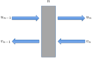
Figure 2: Amplitudes on both sides of the nnth slab. The unitary scattering matrix SS of (6) relates the incoming amplitudes un−1u_{n-1} and vnv_{n} to the outgoing amplitudes unu_{n} and vn−1v_{n-1}, whereas the transfer matrix TT of (8) connects the amplitudes on the left with the amplitudes on the right.

For a wave of wavelength 2​π/k2\pi/k, the wave functions to the left and to the right of the nnth slab are

ψn(left)​(x)\displaystyle\psi_{n}^{\mathrm{(left)}}(x) =\displaystyle= un−1​ei​k​(x−xn)+vn−1​e−i​k​(x−xn),\displaystyle u_{n-1}{\mathrm{e}}^{\mbox{\footnotesize${\mathrm{i}}k(x-x_{n})$}}+v_{n-1}{\mathrm{e}}^{\mbox{\footnotesize$-{\mathrm{i}}k(x-x_{n})$}}\,,
ψn(right)​(x)\displaystyle\psi_{n}^{\mathrm{(right)}}(x) =\displaystyle= un​ei​k​(x−xn−ℓ)+vn​e−i​k​(x−xn−ℓ),\displaystyle u_{n}{\mathrm{e}}^{\mbox{\footnotesize${\mathrm{i}}k(x-x_{n}-\ell)$}}+v_{n}{\mathrm{e}}^{\mbox{\footnotesize$-{\mathrm{i}}k(x-x_{n}-\ell)$}}\,, (5)

where xnx_{n} is the position of the left edge and ℓ\ell is the thickness of the slab; see Fig. 2. The incoming amplitudes are related to the outgoing amplitudes by the unitary scattering matrix SS,

(unvn−1)=S​(un−1vn)=(ab′ba′)​(un−1vn),\left(\begin{array}[]{c}u_{n}\\ v_{n-1}\end{array}\right)=S\left(\begin{array}[]{c}u_{n-1}\\ v_{n}\end{array}\right)=\left(\begin{array}[]{cc}a&b^{\prime}\\ b&a^{\prime}\end{array}\right)\left(\begin{array}[]{c}u_{n-1}\\ v_{n}\end{array}\right), (6)

where the entries of SS are restricted by

|a|2=|a′|2=τ1,|b|2=|b′|2=1−τ1,a∗​b′+b∗​a′=0,|a|^{2}=|a^{\prime}|^{2}=\tau^{\ }_{1}\,,\quad|b|^{2}=|b^{\prime}|^{2}=1-\tau^{\ }_{1}\,,\quad a^{*}b^{\prime}+b^{*}a^{\prime}=0\,, (7)

which account for the single-slab transmission probability τ1\tau_{1}^{\ } and the unitary nature of SS. The particular values of the complex phases of aa, bb, a′a^{\prime}, and b′b^{\prime} are of secondary interest, but we note that we have a=a′=ei​k​ℓ{a=a^{\prime}={\mathrm{e}}^{\mbox{\footnotesize${\mathrm{i}}k\ell$}}} and b=b′=0{b=b^{\prime}=0} for a completely transparent, non-scattering slab, for which ψn(left)​(x)=ψn(right)​(x){\psi_{n}^{\mathrm{(left)}}(x)=\psi_{n}^{\mathrm{(right)}}(x)}.

The transfer matrix TT is used to express the amplitudes on the right in terms of the amplitudes on the left,

(unvn)=T​(un−1vn−1).\left(\begin{array}[]{c}u_{n}\\ v_{n}\end{array}\right)=T\left(\begin{array}[]{c}u_{n-1}\\ v_{n-1}\end{array}\right)\,. (8)

The one-to-one relation between SS and TT implies that the transfer matrix is of the form

T=ei​α​(ei​β00e−i​β)​(cosh⁡θsinh⁡θsinh⁡θcosh⁡θ)​(ei​β′00e−i​β′),T={\mathrm{e}}^{\mbox{\footnotesize${\mathrm{i}}\alpha$}}\left(\begin{array}[]{cc}{\mathrm{e}}^{\mbox{\footnotesize${\mathrm{i}}\beta$}}&0\\[4.30554pt] 0&{\mathrm{e}}^{\mbox{\footnotesize$-{\mathrm{i}}\beta$}}\end{array}\right)\left(\begin{array}[]{cc}\cosh\theta&\sinh\theta\\[4.30554pt] \sinh\theta&\cosh\theta\end{array}\right)\left(\begin{array}[]{cc}{\mathrm{e}}^{\mbox{\footnotesize${\mathrm{i}}\beta^{\prime}$}}&0\\ 0&{\mathrm{e}}^{\mbox{\footnotesize$-{\mathrm{i}}\beta^{\prime}$}}\end{array}\right), (9)

where

cosh⁡θ=1τ1,τ1=2cosh⁡(2​θ)+1,\cosh\theta=\frac{1}{\sqrt{\tau_{1}^{\ }}}\,,\quad\tau_{1}^{\ }=\frac{2}{\cosh(2\theta)+1}\,, (10)

and α\alpha, β\beta, β′\beta^{\prime} are phase factors that have fixed values which, however, are largely irrelevant for what follows.

The transfer matrix for the gap of length LnL_{n} between the nnth slab and the (n+1)(n+1)th slab is the diagonal phase matrix

D⁡(k​Ln)=(ei​k​Ln00e−i​k​Ln).D(kL_{n})=\left(\begin{array}[]{cc}{\mathrm{e}}^{\mbox{\footnotesize${\mathrm{i}}kL_{n}$}}&0\\[4.30554pt] 0&{\mathrm{e}}^{\mbox{\footnotesize$-{\mathrm{i}}kL_{n}$}}\end{array}\right)\,. (11)

Phase matrices of the same structure sandwich the central θ\theta-dependent matrix in (9), so that we have

T=ei​α​D​(β)​t​(θ)​D​(β′)with​t​(θ)=(cosh⁡θsinh⁡θsinh⁡θcosh⁡θ)T={\mathrm{e}}^{\mbox{\footnotesize${\mathrm{i}}\alpha$}}D(\beta)\,t(\theta)\,D(\beta^{\prime})\quad\mbox{with}\enskip t(\theta)=\left(\begin{array}[]{cc}\cosh\theta&\sinh\theta\\[4.30554pt] \sinh\theta&\cosh\theta\end{array}\right) (12)

as a more useful way of writing TT.

The product of two transfer matrices is another transfer matrix, whereby the relevant observation is the composition law

t⁡(θ1)​D​(ϕ)​t​(θ2)=D⁡(γ)​t​(θ1&2)​D​(γ′)t(\theta_{1})\,D(\phi)\,t(\theta_{2})=D(\gamma)\,t(\theta_{1\&2})\,D(\gamma^{\prime}) (13)

with θ1&2\theta_{1\&2} determined by

cosh⁡(2​θ1&2)\displaystyle\cosh(2\theta_{1\&2}) =\displaystyle= cosh⁡(2​θ1)​cosh⁡(2​θ2)\displaystyle\cosh(2\theta_{1})\cosh(2\theta_{2}) (14)
+cos⁡(2​ϕ)​sinh⁡(2​θ1)​sinh⁡(2​θ2)\displaystyle\mbox{}+\cos(2\phi)\sinh(2\theta_{1})\sinh(2\theta_{2})

and the phases γ\gamma and γ′\gamma^{\prime} by

e2​i​γ​sinh⁡(2​θ1&2)\displaystyle{\mathrm{e}}^{\mbox{\footnotesize$2{\mathrm{i}}\gamma$}}\sinh(2\theta_{1\&2}) =\displaystyle= sinh⁡(2​θ1)​cosh⁡(2​θ2)\displaystyle\sinh(2\theta_{1})\cosh(2\theta_{2})
+cos⁡(2​ϕ)​cosh⁡(2​θ1)​sinh⁡(2​θ2)\displaystyle\mbox{}+\cos(2\phi)\cosh(2\theta_{1})\sinh(2\theta_{2})
+i​sin⁡(2​ϕ)​sinh⁡(2​θ2),\displaystyle\mbox{}+{\mathrm{i}}\sin(2\phi)\sinh(2\theta_{2})\,,
e2​i​γ′​sinh⁡(2​θ1&2)\displaystyle{\mathrm{e}}^{\mbox{\footnotesize$2{\mathrm{i}}\gamma^{\prime}$}}\sinh(2\theta_{1\&2}) =\displaystyle= cosh⁡(2​θ1)​sinh⁡(2​θ2)\displaystyle\cosh(2\theta_{1})\sinh(2\theta_{2}) (15)
+cos⁡(2​ϕ)​sinh⁡(2​θ1)​cosh⁡(2​θ2)\displaystyle\mbox{}+\cos(2\phi)\sinh(2\theta_{1})\cosh(2\theta_{2})
+i​sin⁡(2​ϕ)​sinh⁡(2​θ1).\displaystyle\mbox{}+{\mathrm{i}}\sin(2\phi)\sinh(2\theta_{1})\,.

Whereas (15) is of no consequence for the following considerations, the rule (14) is of central importance.

3 Many slabs: A recurrence relation

We now turn to the situation of Fig. 1, where we have NN identical slabs separated by gaps L1L_{1}, L2L_{2}, …, LN−1L_{N-1} that are not controlled on the scale set by the wavelength 2​π/k2\pi/k. Therefore, we regard the phase factors ei​k​Ln{\mathrm{e}}^{\mbox{\footnotesize${\mathrm{i}}kL_{n}$}} as random with a uniform distribution on the unit circle in the complex plane.

The over-all transfer matrix

Ttot\displaystyle T_{\mathrm{tot}} =\displaystyle= TD(kL1)TD(kL2)T⋯TD(kLN−1)T\displaystyle TD(kL_{1})TD(kL_{2})T\cdots TD(kL_{N-1})T (16)
=\displaystyle= ei​N​α​D​(β)​(∏n=1N−1t⁡(θ)​D​(ϕn))​t​(θ)​D​(β′)\displaystyle{\mathrm{e}}^{\mbox{\footnotesize${\mathrm{i}}N\alpha$}}D(\beta)\Biggl(\prod_{n=1}^{N-1}t(\theta)\,D(\phi_{n})\Biggr)t(\theta)\,D(\beta^{\prime})
=\displaystyle= ei​αtot​D​(βtot)​t​(θtot)​D​(βtot′)\displaystyle{\mathrm{e}}^{\mbox{\footnotesize${\mathrm{i}}\alpha_{\mathrm{tot}}$}}D(\beta_{\mathrm{tot}})\,t(\theta_{\mathrm{tot}})\,D(\beta^{\prime}_{\mathrm{tot}})

is characterized by θtot\theta_{\mathrm{tot}} which is obtained by repeated application of the composition rule (14), whereby the phases ϕn=β+β′+k​Ln{\phi_{n}=\beta+\beta^{\prime}+kL_{n}} have random values. Each experimental realization of the NN-slab stack of Fig. 1 has different values for these random phases, and the transmission probability

τN=2cosh⁡(2​θtot)+1\tau_{N}^{\ }=\frac{2}{\cosh(2\theta_{\mathrm{tot}})+1} (17)

varies from one experiment to the next. We need to average over the N−1{N-1} random phases to find ⟨τN⟩{\left\langle\vphantom{\big|}\tau_{N}^{\ }\right\rangle}.

Refer to caption
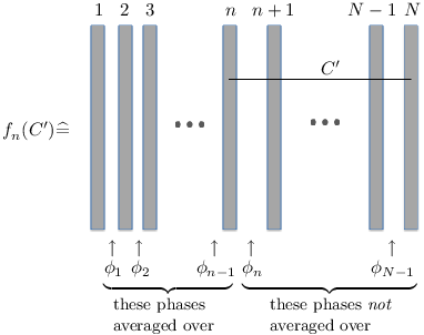
Figure 3: Regarding the meaning of fn​(C′)f_{n}^{\ }(C^{\prime}) in (18) and (19). The random phases ϕ1\phi_{1}, ϕ2\phi_{2}, …, ϕn−1\phi_{n-1} have already been averaged over, but the averaging over the phases ϕn\phi_{n}, …, ϕN−1\phi_{N-1} is yet to be performed.

Let us consider a somewhat more general question: What is the average value ⟨f(cosh(2θtot))⟩{\left\langle\vphantom{\big|}f\bigl(\cosh(2\theta_{\mathrm{tot}})\bigl)\right\rangle} of a function of cosh⁡(2​θtot)\cosh(2\theta_{\mathrm{tot}}), and thus of a function of τN\tau_{N}^{\ }? When the averaging is carried out successively, first averaging over ϕ1\phi_{1}, then over ϕ2\phi_{2}, and so forth, finally over ϕN−1\phi_{N-1}, we have an intermediate value fn​(C′)f_{n}^{\ }(C^{\prime}) after averaging over the first n−1{n-1} random phases; see Fig. 3. Here C′C^{\prime} denotes the value of cosh(2θn⋯N)\cosh(2\theta_{n\cdots N}) for the stack of slabs nn to NN with its dependence on the remaining phases ϕn\phi_{n}, …, ϕN−1\phi_{N-1}. We then have f1​(C′)=f⁡(C′)f_{1}^{\ }(C^{\prime})=f(C^{\prime}) for the value prior to any averaging, and (14) tells us that we get fn+1​(C′)f_{n+1}^{\ }(C^{\prime}) from fn​(C′)f_{n}^{\ }(C^{\prime}) by means of

fn+1​(C′)=∫(2​π)d​φ2​π​fn​(C​C′+S​S′​cos⁡φ)\displaystyle f_{n+1}^{\ }(C^{\prime})=\int\limits_{(2\pi)}\frac{{\mathrm{d}}\varphi}{2\pi}\,f_{n}^{\ }(CC^{\prime}+SS^{\prime}\cos\varphi)
with​C=cosh⁡(2​θ)=2τ1−1,S=sinh⁡(2​θ)=2τ1​1−τ1,\displaystyle\mbox{with}\enskip C=\cosh(2\theta)=\frac{2}{\tau_{1}^{\ }}-1\,,\quad S=\sinh(2\theta)=\frac{2}{\tau_{1}^{\ }}\sqrt{1-\tau_{1}^{\ }}\,,
and​S′=C′2−1with​C′≥1,\displaystyle\mbox{and}\enskip S^{\prime}=\sqrt{{C^{\prime}}^{2}-1}\quad\mbox{with}\enskip C^{\prime}\geq 1\,, (18)

and the integration covers any convenient interval of 2​π2\pi. Eventually this takes us to

⟨f(cosh(2θtot))⟩=fN(C){\left\langle\vphantom{\big|}f\bigl(\cosh(2\theta_{\mathrm{tot}})\bigl)\right\rangle}=f_{N}^{\ }(C) (19)

when the recursive averaging over the N−1{N-1} random phases is completed.

For illustration, we take f1​(C′)=C′f_{1}^{\ }(C^{\prime})=C^{\prime} as a first example. The recurrence relation (18) yields fn​(C′)=Cn−1​C′f_{n}^{\ }(C^{\prime})=C^{n-1}C^{\prime}, so that

⟨cosh⁡(2​θtot)⟩=cosh⁡(2​θ)N{\left\langle\vphantom{\big|}\cosh(2\theta_{\mathrm{tot}})\right\rangle}=\cosh(2\theta)^{N} (20)

or

⟨1/τN⟩=12+12​(2/τ1−1)N{\left\langle\vphantom{\big|}1/\tau_{N}^{\ }\right\rangle}=\frac{1}{2}+\frac{1}{2}(2/\tau_{1}^{\ }-1)^{N} (21)

when stated in terms of transmission probabilities. A second illustrating example is f1​(C′)=C′2−13f_{1}^{\ }(C^{\prime})={C^{\prime}}^{2}-\frac{1}{3}, for which

fn​(C′)\displaystyle f_{n}^{\ }(C^{\prime}) =\displaystyle= [32​f1​(C)]n−1​f1​(C′),\displaystyle\biggl[\frac{3}{2}f_{1}^{\ }(C)\biggr]^{n-1}f_{1}^{\ }(C^{\prime})\,,
fN​(C)\displaystyle f_{N}^{\ }(C) =\displaystyle= 23​[32​f1​(C)]N,\displaystyle\frac{2}{3}\biggl[\frac{3}{2}f_{1}^{\ }(C)\biggr]^{N}\,, (22)

and

⟨cosh(2θtot)2⟩=13+23[12(3cosh(2θ)2−1)]N{\left\langle\vphantom{\big|}\cosh(2\theta_{\mathrm{tot}})^{2}\right\rangle}=\frac{1}{3}+\frac{2}{3}\biggl[\frac{1}{2}\bigl(3\cosh(2\theta)^{2}-1\bigr)\biggr]^{N} (23)

follows.

Taken together, (20) and (23) tell us that the normalized variance of cosh⁡(2​θtot)\cosh(2\theta_{\mathrm{tot}}) grows exponentially with the number of slabs,

⟨cosh⁡(2​θtot)2⟩⟨cosh⁡(2​θtot)⟩2−1\displaystyle\frac{{\left\langle\vphantom{\big|}\cosh(2\theta_{\mathrm{tot}})^{2}\right\rangle}}{{\left\langle\vphantom{\big|}\cosh(2\theta_{\mathrm{tot}})\right\rangle}^{2}}-1 =\displaystyle= 13cosh(2θ)−2​N+23[1+12tanh(2θ)2]N\displaystyle\frac{1}{3}\cosh(2\theta)^{-2N}+\frac{2}{3}\biggl[1+\frac{1}{2}\tanh(2\theta)^{2}\biggr]^{N} (24)
≈\displaystyle\approx 23​[32−12​(τ12−τ1)2]Nfor N≫1.\displaystyle\frac{2}{3}\biggl[\frac{3}{2}-\frac{1}{2}\Bigl(\frac{\tau_{1}^{\ }}{2-\tau_{1}^{\ }}\Bigr)^{2}\biggr]^{N}\quad\mbox{for ${N\gg 1}$.}

The values of τN\tau^{\ }_{N} cover a correspondingly large range, and so we understand why the two sides of (2) differ by much.

This brings us to the much more important log⁡τ\log\tau case of

f1​(C′)=log⁡2C′+1.f_{1}^{\ }(C^{\prime})=\log\frac{2}{C^{\prime}+1}\,. (25)

Here,

fn​(C′)=(n−1)​f1​(C)+f1​(C′),fN​(C)=N​f1​(C)f_{n}^{\ }(C^{\prime})=(n-1)f^{\ }_{1}(C)+f^{\ }_{1}(C^{\prime})\,,\quad f^{\ }_{N}(C)=Nf_{1}(C) (26)

is a manifestation of the “self-averaging” of the logarithm (not any logarithm though, but this particular one), and we get

⟨log⁡2cosh⁡(2​θtot)+1⟩=fN​(C)=N​log⁡τ1.{\left\langle\vphantom{\big|}\log\frac{2}{\cosh(2\theta_{\mathrm{tot}})+1}\right\rangle}=f^{\ }_{N}(C)=N\log\tau_{1}^{\ }\,. (27)

This is the Berry–Klein result (1), of course.

Finally, we turn to calculating ⟨τN⟩{\left\langle\vphantom{\big|}\tau^{\ }_{N}\right\rangle}. The first few fn​(C′)f_{n}^{\ }(C^{\prime})s are

f1​(C′)\displaystyle f_{1}(C^{\prime}) =\displaystyle= 2C′+1,\displaystyle\frac{2}{C^{\prime}+1}\,,
f2​(C′)\displaystyle f_{2}(C^{\prime}) =\displaystyle= 2C′+C,\displaystyle\frac{2}{C^{\prime}+C}\,,
f3​(C′)\displaystyle f_{3}(C^{\prime}) =\displaystyle= 2(C′+1)​(2​C2+C′−1),\displaystyle\frac{2}{\sqrt{(C^{\prime}+1)(2C^{2}+C^{\prime}-1)}}\,, (28)

giving

⟨τ2⟩=f2​(C)=1C=τ12−τ1,\displaystyle{\left\langle\vphantom{\big|}\tau_{2}^{\ }\right\rangle}=f_{2}^{\ }(C)=\frac{1}{C}=\frac{\tau_{1}^{\ }}{2-\tau_{1}^{\ }}\,,
⟨τ3⟩=f3​(C)=2(C+1)​2​C−1=τ14/τ1−3,\displaystyle{\left\langle\vphantom{\big|}\tau_{3}^{\ }\right\rangle}=f_{3}^{\ }(C)=\frac{2}{(C+1)\sqrt{2C-1}}=\frac{\tau_{1}^{\ }}{\sqrt{4/\tau_{1}^{\ }-3}}\,, (29)

and it is frustratingly difficult to go beyond n=3n=3. But it is possible to evaluate the recurrence relation (18) numerically and so determine ⟨τN⟩=fN​(C){\left\langle\vphantom{\big|}\tau^{\ }_{N}\right\rangle}=f^{\ }_{N}(C). In passing, we note that ⟨τ2⟩ray=⟨τ2⟩{\left\langle\vphantom{\big|}\tau_{2}^{\ }\right\rangle}^{\ }_{\mathrm{ray}}={\left\langle\vphantom{\big|}\tau_{2}^{\ }\right\rangle} and ⟨τ3⟩ray>⟨τ3⟩{\left\langle\vphantom{\big|}\tau_{3}^{\ }\right\rangle}^{\ }_{\mathrm{ray}}>{\left\langle\vphantom{\big|}\tau_{3}^{\ }\right\rangle} for 0<τ1<1{0<\tau_{1}^{\ }<1}; ray optics fails for N>2{N>2}.

Refer to caption
Figure 4: Average transmission probability for a stack of NN identical slabs. For τ1=0.85\tau_{1}^{\ }=0.85 and N≤200{N\leq 200}, the dotted curve ‘a’ shows the values of log⁡⟨τN⟩\log{\left\langle\vphantom{\big|}\tau_{N}^{\ }\right\rangle} computed by a numerical evaluation of the recurrence relation (18), commencing with the small-nn functions of (28). The crosses that follow curve ‘a’ are values obtained by a Monte Carlo calculation that simulated 400,000400,000 experimental realizations. The two solid lines are the upper and lower bounds of (32) and (36), respectively. The dashed line ‘b’ is the lower bound (3) derived by Berry and Klein [3].

For τ1=0.85\tau_{1}^{\ }=0.85, the outcome of such a computation is shown in the lin-log plot of Fig. 4 as the dotted curve ‘a’. The crosses near the curve were obtained by a Monte Carlo calculation in which 400,000400,000 experiments were simulated with up to 200200 slabs. The straight dashed line ‘b’ is the lower bound of (3). The solid lines are the upper and lower bounds discussed in the next section. Other values of τ1\tau_{1}^{\ } result in plots with the same general features.

4 Many slabs: Upper and lower bounds

Since f2​(C′)≤1/C′​Cf_{2}^{\ }(C^{\prime})\leq 1/\sqrt{C^{\prime}C}, we have

f3​(C′)\displaystyle f_{3}^{\ }(C^{\prime}) ≤\displaystyle\leq 1C′​C​∫(2​π)d​φ2​π​1C+S⁡(S′/C′)​cos⁡φ\displaystyle\frac{1}{\sqrt{C^{\prime}C}}\int\limits_{(2\pi)}\frac{{\mathrm{d}}\varphi}{2\pi}\,\frac{1}{\sqrt{C+S\,(S^{\prime}/C^{\prime})\cos\varphi}} (30)
≤\displaystyle\leq 1C′​C​∫(2​π)d​φ2​π​1C+S​cos⁡φ\displaystyle\frac{1}{\sqrt{C^{\prime}C}}\int\limits_{(2\pi)}\frac{{\mathrm{d}}\varphi}{2\pi}\,\frac{1}{\sqrt{C+S\cos\varphi}}
=\displaystyle= 1C′​C​Υ​(τ1),\displaystyle\frac{1}{\sqrt{C^{\prime}C}}\Upsilon(\tau_{1}^{\ })\,,

where the second inequality recognizes that the integral in the first line is a monotonically increasing function of S′/C′S^{\prime}/C^{\prime}, so that the replacement S′/C′→1S^{\prime}/C^{\prime}\to 1 increases its value. The integral defining Υ⁡(τ1)\Upsilon(\tau_{1}^{\ }) is of elliptic kind and its value is less than 11 if C>1C>1, that is: Υ⁡(τ1)<1\Upsilon(\tau_{1}^{\ })<1 if τ1<1\tau^{\ }_{1}<1. We conclude by induction that

fn​(C′)≤1C′​C​Υ​(τ1)n−2f_{n}^{\ }(C^{\prime})\leq\frac{1}{\sqrt{C^{\prime}C}}\Upsilon(\tau_{1}^{\ })^{n-2} (31)

holds for n≥2n\geq 2. The upper bound

⟨τN⟩≤⟨τ2⟩​Υ​(τ1)N−2{\left\langle\vphantom{\big|}\tau^{\ }_{N}\right\rangle}\leq{\left\langle\vphantom{\big|}\tau^{\ }_{2}\right\rangle}\Upsilon(\tau_{1}^{\ })^{N-2} (32)

then follows. The ray-optics result (4) is inconsistent with this upper bound. Figure 5 shows Υ⁡(τ1)\Upsilon(\tau_{1}^{\ }) as a function of τ1\tau_{1}^{\ }.

Refer to caption
Figure 5: Upper bound Υ⁡(τ1)\Upsilon(\tau_{1}^{\ }) and lower bound Λ⁡(τ1)\Lambda(\tau_{1}^{\ }) on (⟨τN⟩/⟨τ2⟩)1/(N−2)({{\langle\tau^{\ }_{N}\rangle}}/{{\langle\tau^{\ }_{2}\rangle}})^{1/(N-2)} as functions of τ1\tau_{1}^{\ }. The dashed straight line is the lower bound on ⟨τN⟩1/N{\langle\tau^{\ }_{N}\rangle}^{1/N} of (3).

We derive a lower bound by first observing that

f3​(C′)≥f2​(C′)​Λ​(τ1)f^{\ }_{3}(C^{\prime})\geq f^{\ }_{2}(C^{\prime})\Lambda(\tau^{\ }_{1}) (33)

with

Λ⁡(τ1)=minC′⁡f3​(C′)f2​(C′)={12−τ1​forτ1≥2−2τ1−τ12/4​forτ1≤2−2\Lambda(\tau^{\ }_{1})=\min_{C^{\prime}}\frac{f^{\ }_{3}(C^{\prime})}{f^{\ }_{2}(C^{\prime})}=\left\{\begin{array}[]{c@{\ \mbox{for}\ }l}\displaystyle\frac{1}{2-\tau^{\ }_{1}}&\tau_{1}\geq 2-\sqrt{2}\\[12.91663pt] \sqrt{\tau_{1}^{\ }-\tau_{1}^{2}/4}&\tau_{1}^{\ }\leq 2-\sqrt{2}\end{array}\right. (34)

and then inferring by induction that

fn​(C′)≥f2​(C′)​Λ​(τ1)n−2f^{\ }_{n}(C^{\prime})\geq f^{\ }_{2}(C^{\prime})\Lambda(\tau^{\ }_{1})^{n-2} (35)

holds for n≥2n\geq 2. The lower bound

⟨τN⟩≥⟨τ2⟩​Λ​(τ1)N−2{\left\langle\vphantom{\big|}\tau^{\ }_{N}\right\rangle}\geq{\left\langle\vphantom{\big|}\tau^{\ }_{2}\right\rangle}\Lambda(\tau^{\ }_{1})^{N-2} (36)

then follows. The plot of Λ⁡(τ1)\Lambda(\tau_{1}^{\ }) as a function of τ1\tau_{1}^{\ } in Fig. 5 shows that Λ⁡(τ1)>τ1{\Lambda(\tau^{\ }_{1})>\tau^{\ }_{1}} for 0<τ1<1{0<\tau^{\ }_{1}<1} and, therefore, this lower bound is more stringent than (3), but it is not tight either. We are certain, however, that ⟨τN⟩{\left\langle\vphantom{\big|}\tau^{\ }_{N}\right\rangle} is bounded exponentially both from above and from below.

Figure 6 illustrates the two bounds

Λ⁡(τ1)≤(⟨τN⟩⟨τ2⟩)1/(N−2)≤Υ⁡(τ1)\Lambda(\tau^{\ }_{1})\leq\Biggl(\frac{{\left\langle\vphantom{\big|}\tau^{\ }_{N}\right\rangle}}{{\left\langle\vphantom{\big|}\tau^{\ }_{2}\right\rangle}}\Biggr)^{1/(N-2)}\leq\Upsilon(\tau^{\ }_{1}) (37)

for τ1=0.85{\tau^{\ }_{1}=0.85}. The values for curve ‘a’ are obtained by the numerical evaluation of the recurrence relation (18). Clearly all values are well within the two bounds, the horizontal dashed lines. This figure, and analogous plots for other values of τ1{\tau^{\ }_{1}}, suggest that

(⟨τN⟩⟨τ2⟩)1/(N−2)⟶Υ⁡(τ1)as N→∞.\Biggl(\frac{{\left\langle\vphantom{\big|}\tau^{\ }_{N}\right\rangle}}{{\left\langle\vphantom{\big|}\tau^{\ }_{2}\right\rangle}}\Biggr)^{1/(N-2)}\longrightarrow\Upsilon(\tau^{\ }_{1})\quad\mbox{as $N\to\infty$}\,. (38)

The corresponding observation in Fig. 4 is that, for sufficiently large NN, line ‘a’ there is parallel to the solid line for the upper bound. At present, (38) is no more than a conjecture that is supported by a body of numerical evidence.

Refer to caption
Figure 6: Values of (⟨τN⟩/⟨τ2⟩)1/(N−2)({{\langle\tau^{\ }_{N}\rangle}}/{{\langle\tau^{\ }_{2}\rangle}})^{1/(N-2)} for τ1=0.85{\tau^{\ }_{1}=0.85}. The bounds of (37) are the two horizontal dashed lines. Curve ‘a’ shows the actual values. The extrapolation explained in the context of (38) and (39) gives curve ‘b’.

Some of the evidence is curve ‘b’ in Fig. 6. Its values are obtained by an extrapolation that assumes that

(⟨τN⟩⟨τ2⟩)1/(N−2)≈A−B/N\Biggl(\frac{{\left\langle\vphantom{\big|}\tau^{\ }_{N}\right\rangle}}{{\left\langle\vphantom{\big|}\tau^{\ }_{2}\right\rangle}}\Biggr)^{1/(N-2)}\approx A-B/N (39)

for large NN with AA and BB slowly varying with NN. For two consecutive NN values of curve ‘a’ we can get an estimate of AA and BB, and curve ‘b’ represents the successive values of AA thus extrapolated. The rapid and consistent approach of ‘b’ to the horizontal line of the upper limit feeds the expectation that the conjecture (38) could be true. We leave the matter at that.

5 Summary

We established the recurrence relation (18) that facilitates the calculation of the average value ⟨f⁡(τN)⟩{\left\langle\vphantom{\big|}f(\tau_{N}^{\ })\right\rangle} of any function of τN\tau_{N}^{\ }, the transmission probability through the stack of NN identical slabs with random gaps between them. We observed that the individual values of τN\tau_{N}^{\ } are spread over a large range and, therefore, ⟨τN⟩{\left\langle\vphantom{\big|}\tau_{N}^{\ }\right\rangle} exceeds e⟨log⁡τN⟩=τ1N{\mathrm{e}}^{\mbox{\footnotesize${\langle\log\tau_{N}^{\ }\rangle}$}}=\tau_{1}^{N} by much.

Further, we derived strict upper and lower bounds on ⟨τN⟩{\left\langle\vphantom{\big|}\tau_{N}^{\ }\right\rangle}, both bounds being exponential functions of NN. The ray-optics prediction for ⟨τN⟩{\left\langle\vphantom{\big|}\tau_{N}^{\ }\right\rangle} is consistent with the lower bound but not with the upper bound. The upper bound, when used as an approximation for ⟨τN⟩{\left\langle\vphantom{\big|}\tau_{N}^{\ }\right\rangle}, is of much better accuracy than its derivation suggests and, based on numerical evidence, we conjecture that it is asymptotically exact.

Acknowledgments

We are grateful for discussions with Dominique Delande. Centre for Quantum Technologies is a Research Centre of Excellence funded by Ministry of Education and National Research Foundation of Singapore.

References

References

  • [1] Stokes G G 1862 Proc. R. Soc.11 545
  • [2] Buchwald J Z 1989 The Rise of the Wave Theory of Light: Optical Theory and Experiment in the Early Nineteenth Century (Chicago: University of Chicago Press)
  • [3] Berry M V and Klein S 1997 Eur. J. Phys.18 222
  • [4] Hecht E and Zajac A 1974 Optics (Reading, MA: Addison-Wesley)
  • [5] Anderson P W, Thouless D J, Abrahams E, and Fisher D S 1980 Phys. Rev. B 22 3519