UTHEP-588
arXiv:0907.5259
A note on string solutions in
Kazuhiro Sakai22 2 sakai@phys-h.keio.ac.jp,
Department of Physics, Keio University
Hiyoshi, Yokohama 223-8521, Japan
Yuji Satoh33 3 ysatoh@het.ph.tsukuba.ac.jp
Institute of Physics, University of Tsukuba
Tsukuba, Ibaraki 305-8571, Japan
Abstract
We systematically search for classical open string solutions in within the general class expressed by elliptic functions (i.e., the genus-one finite-gap solutions). By explicitly solving the reality and Virasoro conditions, we give a classification of the allowed solutions. When the elliptic modulus degenerates, we find a class of solutions with six null boundaries, among which two pairs are collinear. By adding the sector, we also find four-cusp solutions with null boundaries expressed by the elliptic functions.
July 2009
1 Introduction
Classical open string solutions in the anti-de Sitter (AdS) space with null boundaries give the scattering amplitudes in planar super Yang-Mills theory at strong coupling [1] (for a review, see for example, [2]). Because of this, the problem of finding such solutions have attracted much attention [3]-[11]. Though the solution with four null boundaries and cusps is found in [12, 1], finding the solutions with more than four cusps is still challenging. Recently, a prescription to construct multi-cusp solutions is provided in [13]. There, it is also discussed how to compute the scattering amplitudes without using explicit form of the solutions, and this is demonstrated in the case of the eight-cusp solutions. Regarding the numerical multi-cusp solutions, see [6].
With applications to the scattering amplitudes in mind, we discuss the classical open string solutions in . For this purpose, a good starting point would be a general construction of the classical string solutions in [14], where the solutions are expressed by theta functions and integrals defined over the underlying spectral curve. This construction can also be applied to .11 1 For the closed strings in , another general construction is given in [15]. Explicit genus-one finite-gap solutions are discussed in [16]. However, for constructing relatively simple solutions, it may be easier to make an ansatz of the finite-gap form (i.e., the general form implied by [14]), where one regards the periods and the integrals as free paramters, and search for particular solutions which satisfy definite reality, Virasoro and boundary conditions.
In this paper, we take this approach for the genus-one finite-gap solutions (elliptic solutions). We determine the parameters of the solutions by explicitly solving the equations of motion, and the reality and Virasoro conditions. As a result, we give a classification of the allowed genus-one finite-gap solutions. When the elliptic modulus degenerates, we also find a class of solutions with six null boundaries, among which two pairs are collinear. The solutions are expressed simply by hyperbolic and exponential functions, and describe non-flat minimal surfaces in . The analysis can be generalized to the classical string solutions in . By adding , as a simple example, we find four-cusp solutions with null boundaries expressed by elliptic functions.
The rest of this paper is organized as follows. In section 2, starting with the genus-one finite-gap form, we solve the equations of motion and the normalization condition. We then summarize the Virasoro condition and the reality condition. By solving these conditions, we determine the allowed solutions and give a classification in section 3. In section 4, we discuss examples of the solutions. In particular, we present a class of solutions with six null boundaries. In section 5, we analyze the case of the strings in , and find four-cusp solutions expressed by the elliptic functions. We conclude with a discussion in section 6. The appendix includes our conventions and some formulas of the elliptic theta functions.
2 Genus-one finite-gap solutions
We begin with parametrizing the target space by the embedding coordinates in , namely, , , with a constraint
| (2.1) |
They satisfy the equations of motion
| (2.2) |
and the Virasoro constraints
| (2.3) |
The solutions span minimal surfaces in . In the following, we concentrate on the Euclidean world-sheet with . The case of the Lorentzian world-sheet can be discussed similarly.
To find the solutions, we introduce the vector which satisfies
| (2.4) | |||||
| (2.5) | |||||
| (2.6) |
with the self-consistent potential
| (2.7) |
The equations (2.4)-(2.6) are equivalent to (2.1)-(2.3) under the identification , where
As discussed shortly, more general identifications between and are possible.
In the genus-one case, the finite-gap solution to (2.4)-(2.6) takes the form [14]
| (2.13) |
Here,
| (2.14) |
and is the complete elliptic integral of the first kind with the elliptic modulus. are the elliptic theta functions which have the quasi-periods with and . Compared with the standard notation, we have rescaled the argument of the theta functions by . With this convention, for example, and . To make the following expressions simpler, we have shifted by as in (2.14), which results in the combination of and in . Our conventions of the elliptic theta functions are summarized in the appendix.
Other parameters should be determined by imposing appropriate conditions. First, one finds that the normalization condition (2.4) gives
| (2.15) |
for . The case of is discussed later in section 3.3.22 2 In addition, when , some of the expressions below become singular. In the case of , the solution becomes of the exponential type without the theta functions. The case with is treated as a limiting case from . In deriving this, we have used
| (2.16) |
which follow from product identities of .
Next, to consider the equations of motion, we introduce
| (2.17) |
where . With the help of the formula (A.3), one then obtains
| (2.18) | |||||
and similar equations for with replaced by . For these to be equated with , the -dependence should be common to all . This requirement fixes as
| (2.19) |
where is a constant. Substituting these, one obtains
| (2.20) |
On the other hand, the potential in (2.7) is evaluated using the equations for in (2.16). Some computations show that is indeed given by the right-hand side of (2.20), which verifies the equations of motion.
Third, let us turn to the Virasoro condition. Again, after some algebra, one finds that the constraint
| (2.21) |
determines the constant to be
| (2.22) |
whereas the other constraint reads
| (2.23) | |||||
In terms of , this is equivalent to
| (2.24) |
the solutions of which are
| (2.25) |
In each of these three cases, one finds that
| (2.26) |
and
| (2.27) |
The final condition to be imposed is the reality condition, for which we need to know the allowed identifications between and . In order to analyze these, we note that, from and the equations of motion, the two matrices should be related by constant matrices as . This implies that , and that the tangent spaces of and are isomorphic. Since is an matrix, should generically be an element of or . Therefore, there are two cases for the reality condition:
| (2.28) |
(up to the exchange of and ). In each case, the AdS solution is identified with as
up to and transformations, respectively, where . In both cases, the potential takes the form , from which one can read off the conformal factor of the induced metric and hence the curvature of the surface described by the solution.
In the following, we set () in the theta functions to be real, which implies . When is complex, the reality conditions may not be satisfied.
3 Solving reality and Virasoro conditions
In this section, we solve the reality and Virasoro conditions which are listed in the previous section. First, we concentrate on the case where . The other case with is discussed later.
3.1 reality condition
When , the reality condition is (I) in (2.28). For this to be satisfied for arbitrary , the theta functions should be real or purely imaginary (after extracting the exponential factors due to possible shifts in by . This implies that are real or purely imaginary up to the shifts , under which transform as (factor) according to (A.4). Furthermore, since , , we have only to consider as the shifts: other cases reduce to these cases by absorbing the factors into and . Consequently, it is enough to assume that are in the fundamental region spanned by with segments removed.
Therefore, we have four cases of :
| (3.1) | |||
In addition, after the possible shifts of in are taken into account, real solutions for must be transformed into the canonical form where and exponentials in are real. These impose restrictions on .
Let us discuss these conditions in more detail, e.g., in case (2). In this case, is real, which implies and or . When , the shift of results in a constant factor to the ratio of the theta functions, which we absorb into . As for the shift in , extracting it from gives
| (3.2) |
and similarly for with the signs of flipped. The exponent after the shift should be real and thus . Note that , , and the conditions from the equations of motion (2.19) read
| (3.3) |
On the other hand, from the definition of , (2.17), it follows that
| (3.4) |
and hence . For given , the real part of (or ) is determined by the first equation in (3.3), whereas the imaginary part is consistently determined by the second, if
| (3.5) |
with .
Similarly analyzing other cases, we find that the reality condition imposes
| (3.6) |
Applying the value of in (2.26), these are solved in each case, which imposes the following conditions:
- (1)
(i) ; (ii) (no solutions); (iii) .
- (2)
(i) ; (ii) (no solutions); (iii) (automatic).
- (3)
(i) (no solutions); (ii) ; (iii) (no solutions).
- (4)
(i) ; (ii) (automatic) ; (iii) .
In the table, “no solutions” indicates the cases where the solutions do not exit, whereas “automatic” indicates the cases where the reality condition is automatically satisfied and imposes no restrictions. The cases where are diverging have also been excluded. We have also omitted the values of in the above.
We remark that, when considering both and , is common and only the combinations among cases (1) and (2), or (3) and (4) are allowed.
3.2 Virasoro condition
From the discussion in the previous section, we find that there are six cases of the combinations of . In each combination, there are three possibilities of satisfying the Virasoro condition as in (2.25). It is straightforward to write down the explicit from of the condition in each case and check whether it has solutions or not.
For example, when (), the condition of case (i) in (2.25) reads . Since for real , the condition is satisfied only when . When (), the condition of case (i) in (2.25) reads . Since for real , the condition has solutions when .
Repeating similar analysis for all cases, one finds that the Virasoro constraints impose the following conditions:
- 1-1.
(i) ; (ii) or ; (iii) or .
- 2-2.
(i) and ; (ii) ; (iii) .
- 1-2.
(i) (no solutions); (ii) (no solutions); (iii) .
- 3-3.
(i) ; (ii) or ; (iii) or .
- 4-4.
(i) and ; (ii) ; (iii) .
- 3-4.
(i) (no solutions); (ii) ; (iii) (no solutions).
3.3 classification
Combining the tables in the previous two subsections, we can determine the allowed cases and their conditions:
- 1-1.
(i) (no solutions); (ii) (no solutions); (iii) and .
- 2-2.
(i) and ; (ii) (no solutions); (iii) .
- 1-2.
(i) (no solutions); (ii) (no solutions); (iii) and .
- 3-3.
(i) (no solutions); (ii) and ; (iii) (no solutions).
- 4-4.
(i) and ; (ii) ; (iii) (no solutions).
- 3-4.
(i) (no solutions); (ii) and ;
(iii) (no solutions).
We note that the result is symmetric between the real and the imaginary . This is a consequence of the modular transformation with purely imaginary . In fact, one can check that in the first three cases are mapped to the last three, up to certain factors which can be absorbed into the exponential factors and the normalization constants of . Some asymmetries in the intermediate stage of the analysis are due to having started with the fixed exponents in .
From this result, one finds that the allowed solutions fall into three types. One is the solution with and as in 1-2 (iii) and 3-4 (ii). Such solutions are expressed by the elliptic functions, as we initially intended. We call this type of solutions “elliptic solution”.
The second one is the solution with or and . In this case, the elliptic functions degenerate and the solutions become simpler. One has to be a little careful in taking , since are singular, respectively. For as in 3-3 (ii) and 4-4 (ii), is vanishing and reduces to a constant for finite . However, if we take after shifting , which is imaginary in these cases, by , the ratio of ’s becomes a ratio of the hyperbolic functions. For with as in 1-1 (iii) and 2-2 (iii), by making use of the modular transformation , one finds that for finite the ratio of ’s becmes a ratio of the hyperbolic functions. However, if we take after shifting by , which is allowed in these cases, the ratio of ’s becomes a constant. Thus, depending on the way to take the limit, the degenerate solutions reduce to (a) the known solutions with const.(exponentials), or (b) the solutions with (ratio of hyperbolic functions)(exponentials). In the latter case, the potential is not constant, and the minimal surface spanned by is not flat. We call the former type “exponential solution”, and the latter “hyperbolic solution”.
The third type is the solution with , which we have not considered so far, since the normalization condition (2.15) becomes singular. In this case, (2.16) implies that the only possibilities to satisfy the normalization condition of is or , since the -dependence has to be canceled. Thus, cases 2-2 (i), 4-4 (i) are excluded, though we left them in the table taking into account a possibility that they could be regarded as limiting cases. When , the solutions reduce to the exponential type. When , as discussed above, the solutions become of the exponential or the hyperbolic/trigonometric type. In the latter case, it turns out that one has to set to satisfy the normalization condition. In sum, if , only the solutions of the exponential type are allowed.
For or , one may take appropriate limits from the generic cases to write down the solutions. However, it is more straightforward to start with the generic form of the solutions in these cases, and determine them as in section 2.
3.4 case
So far, we have considered the case where . As discussed in section 2, there is another case with . The reality and Virasoro conditions are analyzed similarly.
First, from the reality condition (II) in (2.28), one finds that there are four cases of :
| (3.7) | |||
In addition, the normalization constants should satisfy and the exponentials in and should be complex conjugate to each other (after the possible shifts of in ).
In any of these cases, the combinations of and satisfy the same relations as the corresponding ones in the case. For example, in case , , though have different relations and . Thus, the constraints from the reality condition are the same.
The Virasoro condition is irrelevant of which embedding we use, or . Therefore, the allowed cases are read off from the same table as in the case in section 3.3. In the case, the condition on implies
| (3.8) |
This may give further constraints on the parameters, e.g., on . When and , we need to exchange and . For the Euclidean world-sheet, which results in space-like surfaces, one finds no solutions eventually.
4 Examples of solutions
Our main motivation to studying the AdS string solutions is the application to the scattering amplitudes in the super Yang-Mills theory. With this in mind, we discuss the obtained solutions.
4.1 searching for cusp solutions
Before going into details, let us summarize some general properties of the solutions in relation to the cusp solutions with null boundaries. First, when , the exponential part of is complex and, since, e.g., Re, the solutions are generally rapidly oscillating near the world-sheet boundary . Thus, to search for the cusp solutions, one should look into the case with (unless the world-sheet is consistently restricted). This case also includes oscillating solutions. For example, in case (2) with real in (3.1), the solution has a factor and this is oscillating. In case (1) with real , the solution has an oscillating factor but, since this does not change the sign, the oscillation is harmless (as can be checked by the modular transformation). For imaginary , if the solutions contain the factors of , they oscillate, whereas if the factors are , they do not. The limiting cases with are similarly considered.
Once one finds the solutions which grow large without harmful oscillation near the world-sheet boundary, they are good candidates of the cusp solutions. Though some of the cusps are generally at the infinity in the boundary Poincaré coordinates, , they can be brought to finite points by an transformation:
with . To see this, we trace a contour with a large radius in the world-sheet. Supposed that one of alternatively becomes dominant along the contour, one finds that the contour is mapped to a rectangular in the -plane which has null boundaries and four cusps at . If shows a more intricate behavior, more cusps and null boundaries may appear. We note that one should choose the transformation so that the Poincaré radial coordinate is non-negative: otherwise, the interpretation of the solution in the Poincaré corrdinates may be subtle.
4.2 elliptic solutions
From the discussion in the above, we find that the elliptic solutions in 1-2 (iii) and 3-4 (ii) are harmfully oscillating solutions. However, in the limit for 1-2 (iii) and for 3-4 (ii), they become the exponential or the hyperbolic solutions in which the oscillation disappears. This is because, e.g., for 1-2 (iii), the period of the oscillation is of order , and this is diverging as ; only the strip with the width of order survives after taking the limit. Conversely, this shows that unwanted oscillation might be eliminated by restricting the world-sheet in some region. In our case, simply taking the world-sheet to be the strip does not give cusp solutions with null boundaries, since the two sides of the strip are mapped to the boundary of the surface in which is not null. However, this may be a useful tip to further search for the cusp solutions. These elliptic solutions are regarded as elliptic generalizations of the known exponential solutions.
4.3 degenerate solutions
The degenerate solutions of the hyperbolic/trigonometic type with are new solutions. As mentioned at the end of section 3.3, instead of taking appropriate limits from the generic cases, one may start with the generic form of the solutions in this case,
| (4.6) |
and determine them as in section 2. Indeed, one finds that the normalization condition and the equations of motion give
| (4.7) |
and
| (4.8) |
respectively, whereas the Virasoro condition imposes
| (4.9) |
Since we are interested in the cusp solutions with real , we impose the reality condition , . It turns out that the solutions to the constraints (4.7)-(4.9) are essentially unique (up to conformal transformations of etc.), and given by
| (4.10) |
These give a class of real and non-oscillating solutions of the form,33 3 Shifting the argument of in (4.6) by gives solutions with .
| (4.11) | |||||
where , , and we have assumed . (The case with is similar.) The potential reads
| (4.12) |
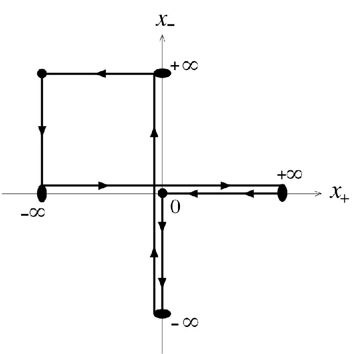
This class of solutions includes solutions which have four cusps, two horns and six null boundaries, among which two pairs are collinear. We remark that all the boundaries are null. To check these properties, we first restrict to the case where so that the Poincaré radial coordinate is non-negative. (In the other case with , we have only to flip the signs of .) Next, we note that the AdS boundary is given by . Plugging the solution (4.11) into , we then find that the world-sheet boundary where or is mapped to the AdS boundary unless . When takes such a generic value, similarly to the discussion in section 4.1 we find that the image of the world-sheet boundary traces six null segments in the -plane. Concretely, the contour with is mapped to as varies from to . The resultant boundary of the surface is not convex, but crossed and folded as in Fig.1. Among the six end-points of the segments, are the cusps and are the tips of the two horns. The essence in producing the six null boundaries is that the change of the sign of “splits” the cusps, which, in the -plane, is observed as the transitions and . In these transitions, the surface boundary has to keep touching the AdS boundary. Since the solution has two pairs of collinear null boundaries, one expects that it gives the scattering amplitudes at strong coupling in a collinear limit.
When , the surface boundaries mapped from do not reach the AdS boundary, and they form two boundaries inside . Consequently, the solution describes a surface which has four null boundaries at the AdS boundary, and two boundaries inside AdS. The surface pinches at a point where these two boundaries intersect each other. The shape of the surface is obtained by diagonally cutting a four-cusp surface and twisting it.
From the potential in (4.12), one finds that the surface has non-trivial curvature. This shows a clear difference from the four-cusp solution in [12, 1], where the potential is constant and hence the corresponding surface is flat. In fact, the two solutions are not related to each other by simple transformations: First, they cannot be related by an transformation, since the potential is invariant. Second, as long as we work with the Euclidean world-sheet, the allowed world-sheet analytic continuation is the continuation of both and , which results in . Thus, is invariant up to a sign and renaming the world-sheet coordinates. Third, one may generate a new solution by a target-space analytic continuation such as together with the world-sheet analytic continuation as in [17]. However, the potential should again be invariant (up to a sign and renaming of the world-sheet coordinates) in order to keep the equations of motion invariant. Finally, if the potential has a factorized form , it may be brought to a constant by a world-sheet conformal transformation, but this is not possible for the degenerate solution.
5 Adding : elliptic four-cusp solutions
The analysis so far can be generalized to the case of the strings in . Here, for simplicity, we consider the case of .
In an appropriate gauge, the field is set to be . The reality of requires . Adding does not change the reality condition on , but that changes the Virasoro constraints to
| (5.1) |
Similarly to the case without , linear combinations of these give
| (5.2) | |||
Because of the change of the Virasoro constraints, the allowed solutions for also change. Though they can be classified as in section 3, we do not go into details. However, we know that, in order to find cusp solutions, we have only to look into the cases without harmful oscillation. Among the elliptic cases, they are 1-1 or 3-3 in section 3.2, which are related to each other by the modular transformation. In the following, we take 3-3. It turns out that this case indeed gives four-cusp solutions with null boundaries which are expressed by the elliptic functions.
For example, for , the Virasoro condition gives and . Further setting , the theta function takes the form . By repeating the shifts in the imaginary direction as in (A.4), one then finds that the ratio of the theta functions shows an exponential behavior . Thus, along a contour with a large radius in the world-sheet, one of alternatively becomes dominant. Since this shows that the mechanism in section 4.1 works in this case, the solution describes a surface with four null boundaries and four cusps. The points of the cusps in the -plane can be brought to finite points as in section 4.1.
Since the Virasoro constraints are changed, the surface spanned by the solution is not necessarily space-like anymore. This can be checked by considering the normal vector to the surface , the norm of which is Evaluating in this example shows that and hence the surface is time-like.
6 Discussion
We have systematically searched for the classical open string solutions in within the genus-one finite-gap solutions, and given a classification of the allowed solutions. When the elliptic modulus degenerates, we have found a class of solutions with six null boundaries, among which two pairs are collinear. Adding to , we have also found solutions expressed by the elliptic functions, which have four cusps and four null boundaries.
The analysis in this paper can straightforwardly be applied to the case with the Lorentzian world-sheet. It may also be useful for studying the classical solutions describing the Wilson loops in the super Yang-Mills theory at strong coupling [18, 19]. The classical open string solutions in are similarly discussed. In particular, for the strings in , we have only to add another pair of . In this case, these are identified with a complex combination of the embedding coordinates in as , and thus the solutions are generally (harmfully) oscillating.
In such oscillating cases, a way to remove the unwanted oscillation is to restrict the world-sheet, as mentioned in section 4.2. Though it is still non-trivial to find desired solutions with cusps and null boundaries, the prescription in [13] suggests that effectively restricting the world-sheet by conformal transformations deserves further consideration.
The essence of the solution with six null boundaries in section 4.3 is the change of the sign of in front of the exponentials, which “splits” the cusps. Similarly, more intricate behavior of the corresponding factors in the higher-genus cases may produce solutions with more null boundaries. It is interesting to consider the relation to the mechanism provided in [13].
Most of the end points of the null segments in our solutions with six null boundaries are located at the infinity of the boundary. Since the surface is space-like, this is inevitable in the boundary. However, it is desirable to bring them to finite points in the boundary by some transformations, as discussed in [13]. This may be a first step toward applications to the scattering amplitudes. We would like to report progress in the analysis of the higher-genus finite-gap solutions, multi-cusp solutions and the applications to the scattering amplitudes, elsewhere.
Appendix
Our conventions of the elliptic theta functions are:
| (A.1) |
and
| (A.2) |
where and is the complete elliptic integral of the first kind.
In the main text, we use the formulas
| (A.3) |
where , and
| (A.4) | |||||
Acknowledgments
We would like to thank D. Bak, S. Hirano, N. Ishibashi, K. Ito, H. Itoyama, C. Kalousios, T. Matsuo and K. Mohri for useful conversations. The work of K.S. and Y.S. is supported in part by Grant-in-Aid for Scientific Research from the Japan Ministry of Education, Culture, Sports, Science and Technology.
References
References
- [1] L. F. Alday and J. M. Maldacena, JHEP 0706 (2007) 064 [arXiv:0705.0303 [hep-th]].
- [2] L. F. Alday and R. Roiban, Phys. Rept. 468 (2008) 153 [arXiv:0807.1889 [hep-th]].
- [3] S. Ryang, Phys. Lett. B 659 (2008) 894 [arXiv:0710.1673 [hep-th]].
- [4] A. Jevicki, K. Jin, C. Kalousios and A. Volovich, JHEP 0803 (2008) 032 [arXiv:0712.1193 [hep-th]].
- [5] D. Astefanesei, S. Dobashi, K. Ito and H. Nastase, JHEP 0712 (2007) 077 [arXiv:0710.1684 [hep-th]].
- [6] S. Dobashi, K. Ito and K. Iwasaki, JHEP 0807 (2008) 088 [arXiv:0805.3594 [hep-th]].
- [7] A. Mironov, A. Morozov and T. N. Tomaras, JHEP 0711 (2007) 021 [arXiv:0708.1625 [hep-th]]; Phys. Lett. B 659 (2008) 723 [arXiv:0711.0192 [hep-th]].
- [8] H. Itoyama, A. Mironov and A. Morozov, Nucl. Phys. B 808 (2009) 365 [arXiv:0712.0159 [hep-th]].
- [9] H. Itoyama and A. Morozov, Prog. Theor. Phys. 120 (2008) 231 [arXiv:0712.2316 [hep-th]].
- [10] C. M. Sommerfield and C. B. Thorn, Phys. Rev. D 78 (2008) 046005 [arXiv:0805.0388 [hep-th]].
- [11] H. Dorn, G. Jorjadze and S. Wuttke, arXiv:0903.0977 [hep-th].
- [12] M. Kruczenski, JHEP 0212 (2002) 024 [arXiv:hep-th/0210115].
- [13] L. F. Alday and J. Maldacena, arXiv:0904.0663 [hep-th]; arXiv:0903.4707 [hep-th].
- [14] I. M. Krichever, Func. An. Apps. 28 (1994) No. 1, 26.
- [15] V. A. Kazakov and K. Zarembo, JHEP 0410 (2004) 060 [arXiv:hep-th/0410105].
- [16] H. Hayashi, K. Okamura, R. Suzuki and B. Vicedo, JHEP 0711 (2007) 033 [arXiv:0709.4033 [hep-th]].
- [17] M. Kruczenski, R. Roiban, A. Tirziu and A. A. Tseytlin, Nucl. Phys. B 791 (2008) 93 [arXiv:0707.4254 [hep-th]].
- [18] J. M. Maldacena, Phys. Rev. Lett. 80 (1998) 4859 [arXiv:hep-th/9803002].
- [19] S. J. Rey and J. T. Yee, Eur. Phys. J. C 22 (2001) 379 [arXiv:hep-th/9803001].