Domain walls, canted states and stripe width variation in ultrathin magnetic films with perpendicular anisotropy
Abstract
Stripe width variation in ultrathin magnetic films is a well known phenomenon still not well understood. We analyze this problem considering a 2D Heisenberg model with ferromagnetic exchange interactions, dipolar interactions and perpendicular anisotropy, relevant e.g. in Fe/Cu(001) films. By extending a classic result of Yafet & Gyorgy (YG) and using Monte Carlo simulations we calculate the complete zero temperature phase diagram of the model. Through this calculation we analyze the correlation between domain walls structure and stripe width variation, as the perpendicular anisotropy changes. In particular, we found evidences that the recently detected canted state becomes the ground state of the system close to the Spin Reorientation Transition (SRT) for any value of the exchange to dipolar couplings ratio. Far away of the SRT the canted ground state is replaced by a saturated stripes state, in which in–plane magnetization components are only present inside the walls. We find that the domain wall structure strongly depends on the perpendicular anisotropy: close to SRT it is well described by YG approximation, but a strong departure is observed in the large anisotropy limit. Moreover, we show that stripe width variation is directly related to domain wall width variation with the anisotropy.
Keywords:
ultrathin magnetic films, Heisenberg model, stripe widthpacs
75.40.Gb, 75.40.Mg, 75.10.HI Introduction
Pattern formation in ferromagnetic thin films with perpendicular anisotropy and its thermodynamical description have been the subject of intense experimental [1, 2, 3, 4, 5, 6, 7, 8, 9, 10, 11], theoretical [12, 13, 14, 15, 16, 17, 18, 19, 20] and numerical [21, 22, 23, 24, 25, 26, 27, 28, 29, 30] work in the last 20 years. Magnetic order in ultrathin ferromagnetic films is very complex due to the competition between exchange and dipolar interactions on different length scales, together with a strong influence of shape and magnetocrystalline anisotropies of the sample. These in turn are very susceptible to the growth conditions of the films [8, 31].
Among the different magnetization patterns that have been observed in these systems, striped order (i.e., modulated patterns of local perpendicular magnetization with a well defined half-wavelength or stripe width ) at low temperatures is an ubiquitous phenomenon. One intriguing fact is the strong variation displayed by the equilibrium stripe width in many of these systems, when either the temperature or the film thickness is changed[3, 7, 4, 5, 9, 10]. The origin of such variation is still controversial, but recent results suggest that a key point to understand it is the role played by the interfaces (i.e., the domain walls) between stripes[9]. Thus, a starting point to study this problem is to compare the energies of striped patterns with different domain wall configurations. An accurate description of the domain walls requires to take into account not only the perpendicular component of the local magnetization, but also the in–plane component. Indeed, some experimental results[4] are consistent with the presence of Bloch domain walls, as expected for perpendicularly oriented magnetization domains[32].
To compute the energy contribution of domain walls it is important to consider explicitly the out of plane anisotropy, together with the exchange and dipolar interactions, whose competition is the responsible for the appearance of striped patterns. A minimum model that contains all these ingredients is the 2D dimensionless Heisenberg Hamiltonian:
| (1) |
where are classical unit vectors, the exchange and anisotropy constants are normalized relative to the dipolar coupling constant (), stands for a sum over nearest neighbors pairs of sites in a square lattice, stands for a sum over all distinct pairs and is the distance between spins and .
In the large anisotropy limit this model reduces to an Ising model with short range ferromagnetic and long range antiferromagnetic interactions, whose ground state is the striped one[25]. In that limit the stripe width increases exponentially with the exchange to dipolar coupling ratio[21, 26] . For low values of the anisotropy, the ground state of this model changes to a planar ferromagnetic state[13]. In a classic work, Yafet and Gyorgy computed the energy of striped domain configurations with Bloch domain walls, by considering a sinusoidal (perpendicular) magnetization profile at the walls and saturated magnetization inside the stripes[13]. They found that above certain threshold value a striped configuration has less energy than a uniformly (in–plane) magnetized one. At this point the system shows a Spin Reorientation Transition (SRT). Also within this approximation the stripe width shows an exponential increase with the anisotropy strength, while the domain wall width decreases algebraically for large enough values of , at least for large values of . This approximation is expected to work well close to the SRT, where the effective anisotropy is small[18]. However, for large values of and not too close to the SRT (i.e., when the width of both stripes and walls are large) one can expect a large departure in the wall energy contribution with respect to the true domain wall configuration, which should approach a hyperbolic tangent profile[32].
Another important point concerns the in–plane magnetization component inside the stripes. In their work Yafet and Gyorgy considered striped solutions where the only in–plane components lay inside the walls, although they pointed out how to extend their calculations to consider non–saturated magnetization inside the stripes[13]. Based on that calculation, Politi[18] reported that, at least for large enough values of , the magnetization should show an abrupt saturation very close to the SRT, suggesting that the in–plane component inside the stripes is not relevant. However, recently Whitehead et al[30] obtained evidences of a non–saturated ground state at a relatively small value of for a wide range of values of the anisotropy strength . Their numerical results also showed a correlation between the stripe width and the in–plane component variations and suggest that this ground state configuration stabilizes at finite temperature, giving rise to what they called a “canted" phase. Hence, it is important to revise the zero temperature phase diagram of this model in the whole space, including canted configurations, in order to determine to what extent they can be relevant to real systems and their possible influence to the stripe width variation phenomenon.
It is worth noting that the perpendicular anisotropy changes (inversely) with the film thickness[29]. It has also been pointed out that the changes in the film thickness can act as a change in the effective temperature[3]. Hence, understanding the variation of the equilibrium stripe width and the associated domain wall structure as the anisotropy changes at zero temperature can be of great help to understand the corresponding properties a finite temperature, a far more complex problem.
In this work we analyze the complete equilibrium phase diagram at zero temperature in the space of Hamiltonian (1). Following Yafet and Gyorgy’s work, we only consider straight domains, i.e., domains in which the spin orientation can be modulated along the direction but is constant in the perpendicular direction ( are the coordinates on the plane of the film ). We also consider only Bloch walls, i.e., walls in which the magnetization stays inside the plane. In order to clarify notation and units, and to include some extensions, we briefly review Yafet & Gyorgy’s approximation in Appendix A. To obtain the phase diagram we compute the energy of different types of magnetization profiles and compare them with simulation results obtained through a zero temperature Monte Carlo (MC) method specially designed for the present purposes. The MC method is presented in Appendix C. In section II we derive a general expression for the energy of striped magnetization profiles. The zero temperature phase diagram and associated properties are derived in section III. A discussion and conclusions are presented in section IV.
II Energy of striped magnetization profiles
Let us consider a square lattice with sites, characterized by the integer indexes , where and , in the limit . Hence, the index in Eq.(1) denotes a pair of coordinates . Following YG approximation[13], we consider only uniformly magnetized solutions along every vertical line of sites, i.e. , and allow only Bloch walls between domains of perpendicular magnetization, i.e. . Therefore,
| (2) |
Then, for every value of there is only one independent component of the magnetization.
YG showed that for these types of spin configurations the energy per spin can be mapped onto the energy of a one dimensional XY model. The energy difference between an arbitrary magnetization profile and a uniformly in–plane magnetized state is then given by (see Appendix A.1):
| (3) |
where , , , , and
| (4) |
Although small, this correction term makes a non negligible contribution when the domain walls are of the same order of the lattice constant. This happens for small values of (), where both the stripe and wall widths are of the order of a few lattice spacings. For larger values of it is reasonable to assume a smooth magnetization profile[13] , so that
| (5) |
can be absorbed into the anisotropy term in Eq.(3), replacing .
Considering now a stripe-like periodic structure of the magnetization profile with period , i.e.
| (6) |
we can make use of a Fourier expansion:
| (7) |
where we have assumed an even function of just for simplicity.
The anisotropy term in Eq.(3) can be written as
| (8) |
and the dipolar term[13]
| (9) |
where[33]
| (10) |
In the general case, it is better to let the exchange term (and the correction term as well) in Eq.(3) expressed in terms of the angle between and the axis:
| (11) | |||||
| (12) |
where the angle has the same periodicity of . We have that
| (13) |
Putting all the terms together we get the general expression:
| (14) |
III Zero temperature phase diagram
In this section we look for the minimum of Eq.(14) for different values of . We propose different striped magnetization profiles and compare the energies obtained by minimizing Eq.(14) for each profile with respect to variational parameters.
III.1 Small values of : Sinusoidal Wall magnetization Profile (SWP) approximation
We first consider a profile as proposed by YG, that is constant inside the stripes and has a sinusoidal variation inside the walls between stripes (see Fig.1 in Ref. 13):
| (15) |
where is the absolute value of magnetization inside the stripes and is the wall width. In order to allow for canted profiles, we take , where is the canted angle, i.e. we define it as the minimum angle of the local magnetization with respect to the axis. Yafet and Gyorgy solved this variational problem for in the continuum limit[13], i.e. when and , so that the profile can be considered a smooth function of . While this approximation is expected to work well for large enough values of , it breaks down for relatively small values of it, where the discrete character of the lattice has to be taken into account. However, the variational problem for that range of values of can be solved exactly (although numerically) by minimizing Eq.(14) with respect to the integer variational parameters and and continuous parameter . In other words, for every pair of values we evaluate the energy Eq.(14) for the profile (15) with different combinations of and within a limited set. For every pair of values ,we look for the value of that minimizes the energy with a resolution and compare all those energies. Details of that evaluation are given in Appendix B. This calculation is feasible for values up to , for which the maximum value of (bounded by the stripe width in the limit) remains relatively small (smaller than ). Some results for close to the SRT were also obtained. All the results of this calculation are compared against Monte Carlo (MC) simulations. Details of the MC method used are given in Appendix C. Through these calculations we obtain a zero temperature phase diagram for low values of .
Before presenting the results, it is important to introduce some notations and definitions of different types of solutions. We distinguish between four types of solutions. If the minimum energy solution corresponds to and (within the resolution ), we call this a Striped Ising Profile (SIP), i.e. a square wave like profile. If but , we call this a Saturated State. These states show a finite parallel component of the magnetization inside the walls. If the solution is a Canted State. Finally, if () we have a Planar Ferromagnet (PF).
The zero temperature phase diagram for small values of () is shown in Fig.1. For relatively large values of the minimum energy configuration is always the Ising one (SIP), with a stripe width independent of . For small values of the minimum energy configuration is the PF, with a spin reorientation transition line (SRT), either to the Ising state for () or to a canted one for (). No Saturated State configurations are observed for .
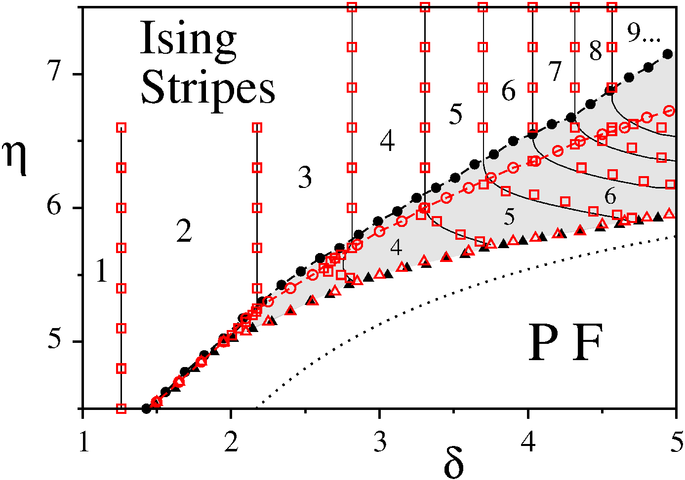
Inside the canted region, a strong stripe width variation with the anisotropy is observed at constant . Note that the vertical lines that separate Ising striped states with consecutive values of bend inside the canted region and become almost horizontal as increases. Hence, the exponential increase of with in the Ising region (vertical lines) changes to an exponential increase with deep inside the canted region (curved lines on the right of Fig.1).
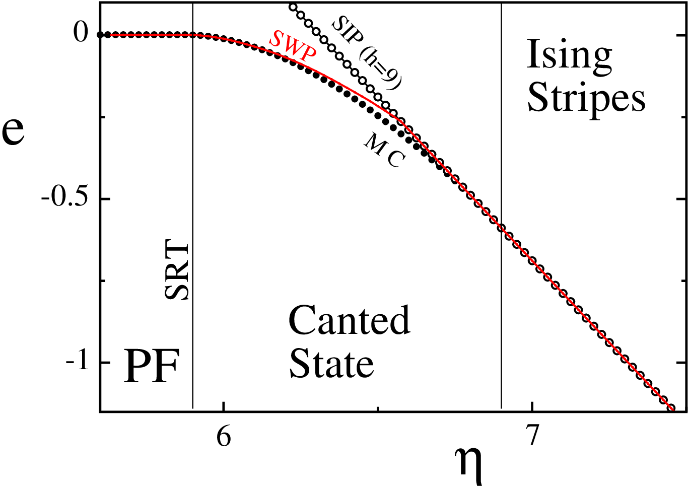
We also find an excellent agreement between the sinusoidal wall profile approximation and the MC results, except close to the transition between the Ising and the canted states. Such disagreement is due to the fact that the actual wall is not well described by a sinusoidal profile far away of the SRT line, as will be shown later. In Fig.2 we show a comparison between the energy of the SWP and the MC results as a function of for . The range of values of where the walls are not well described by a sinusoidal profile increases with .
For large enough values of the variational problem for the SWP can be solved in a continuum approximation introduced by YG[13]. This leads to the equations (see Appendix A.2):
| (16) | |||||
| (17) | |||||
| (18) |
where , and . In the limit (pure sinusiodal profile) these equations can be solved analytically and predict a SRT at the line
| (19) |
with (see Appendix A.2). The line Eq.(19) is also depicted in Fig.1. Notice the disagreement between the continuum approximation and the exact one for . This discrepancy becomes smaller than only for .
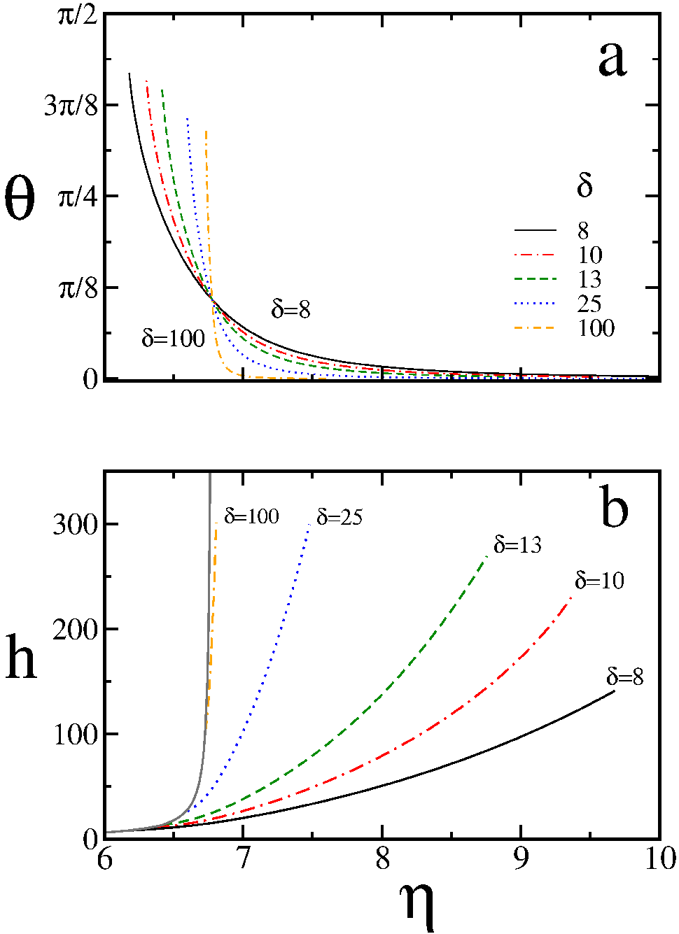
For arbitrary values of and Eqs.(16)-(18) can be solved numerically. In Fig.3 we show the numerical solutions for and as a function of for different values of . We see that the range of values of the anisotropy for which the canted angle is appreciable different from zero within this approximation is strongly depressed as increases. For values the canted configuration almost disappears, except very close to the reorientation line, consistently with the results reported by Politi[18].
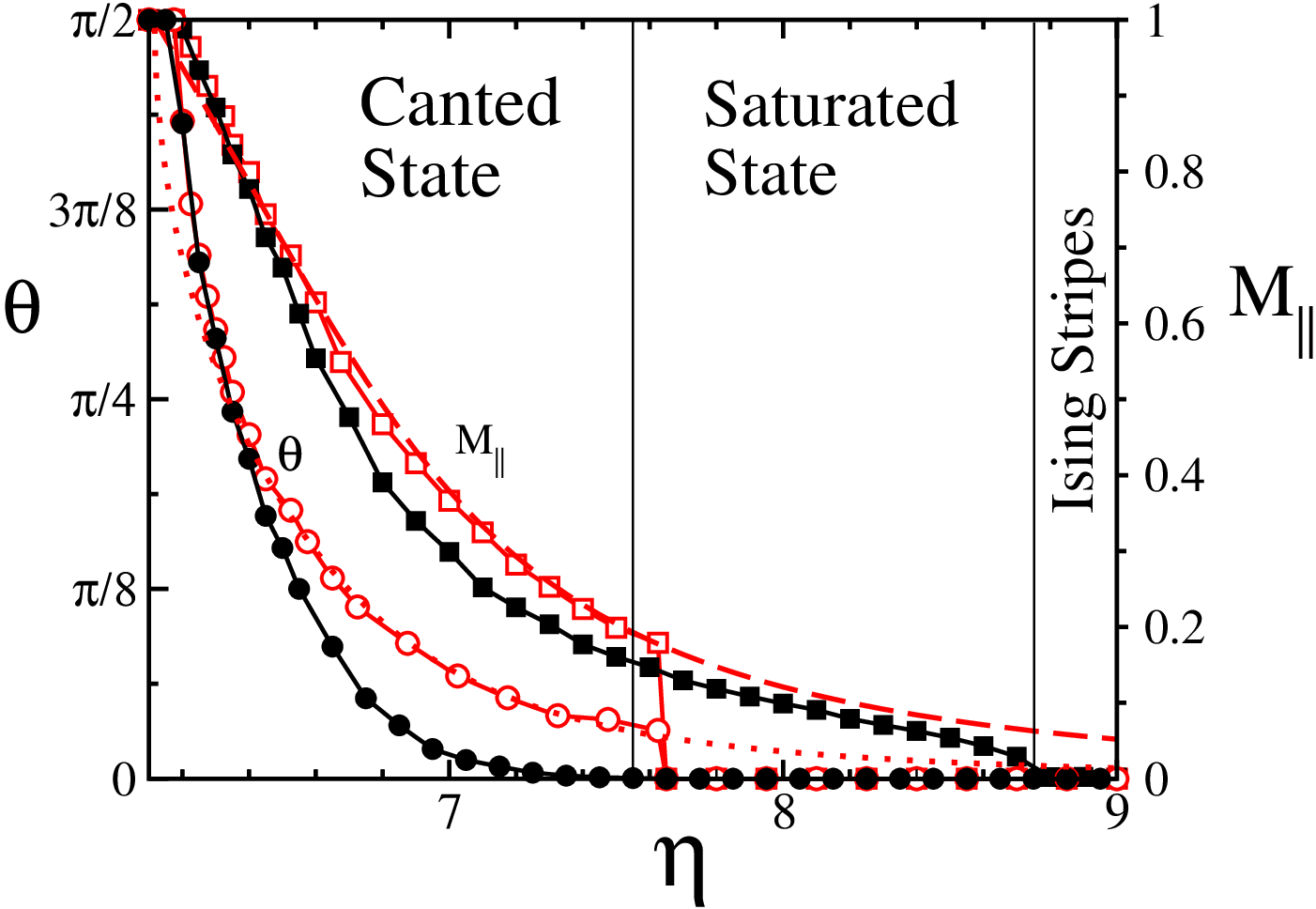
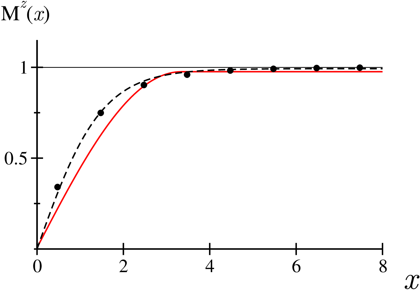
Indeed, from our MC simulations, we observe that the range of values for which the canted state has the minimum energy gradually shrinks as increases, being replaced by a saturated state for values of above certain threshold. This can be observed in Fig.4, where we show the behavior of the canted angle and the in–plane magnetization component as a function of for . The Monte Carlo data shows the existence of a wide range of values of for which the canted angle is zero while , meaning that the non null in–plane components are concentrated inside the walls. In other words, in that region we have a saturated state with thick walls . Notice also that the SWP approach completely fails to describe those states. Moreover, we observe from our MC simulations that the SWP cease to be the minimum energy solution for values of relatively close to the SRT, well before the saturated state sets up (see Fig.4). This effect becomes more marked as increases.
III.2 Large values of : Hyperbolic Wall magnetization Profile (HWP) approximation
As already pointed out, the actual magnetization profile departs from the SWP for large values of and . This is expected from micromagnetic theory, which in that limit predicts that the wall structure will be dominated by the interplay between anisotropy and exchange, leading to an hyperbolic tangent shape of the wall[32]. This can be observed in Fig.5. Hence we considered a periodic magnetization profile with hyperbolic tangent walls (HWP) defined, for a wall centered at , by
| (20) |
together with Eq.(6) where as before. In the large limit, assuming a smooth profile and , the anisotropy energy can be expressed as:
| (21) | |||||
The exchange energy can be obtained in a similar way:
| (22) | |||||
Solving the last integral we finally obtain
| (23) |
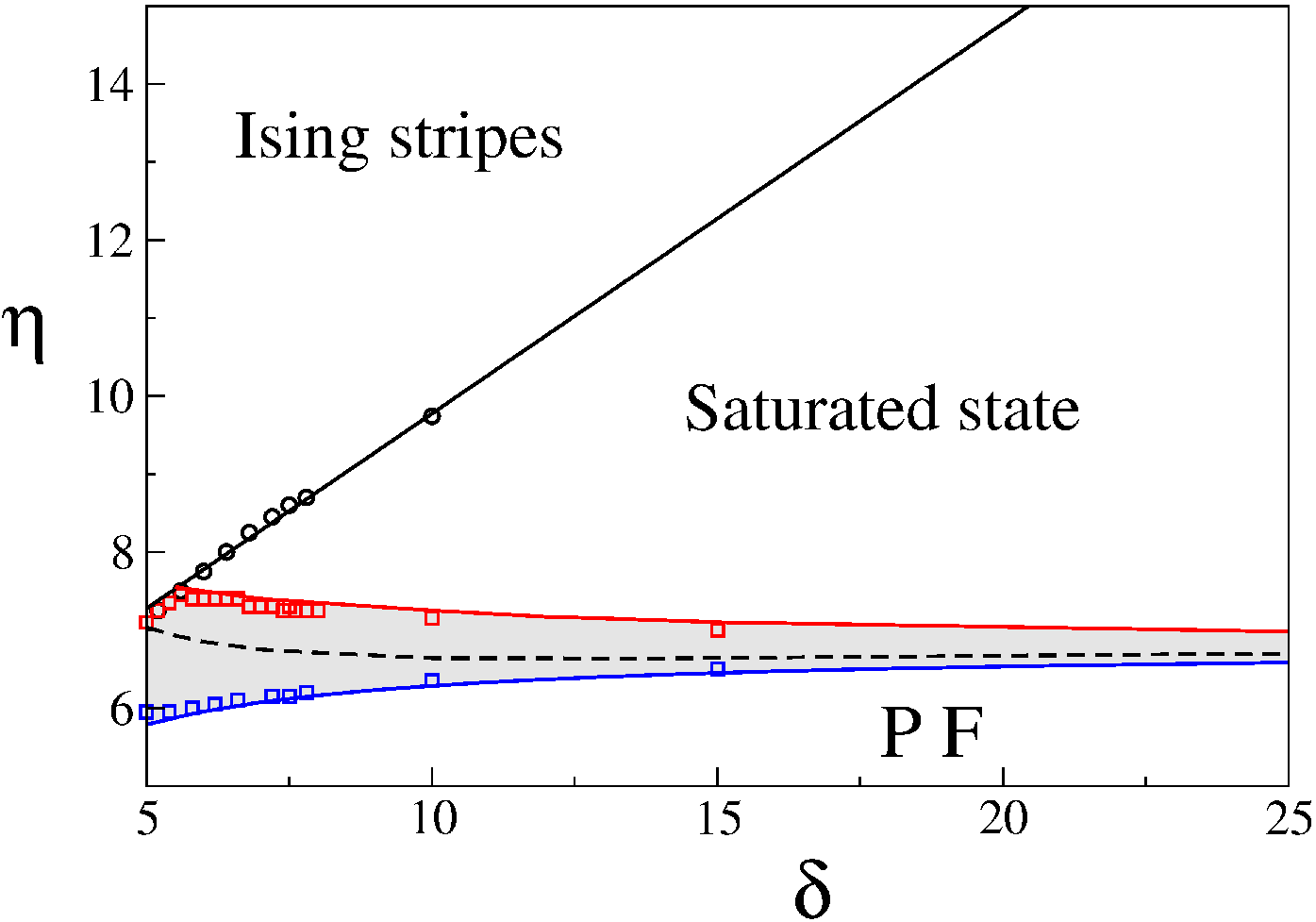
The dipolar energy can be calculated using Eqs.(9) and (10). The Fourier coefficients for the profile (20) can be computed using the approximation (68) (see Appendix D). This leads to an expression for the total energy as a function of the variational parameters , and that can be minimized numerically. Comparing the minimum energy solution for the SWP and the HWP we obtain the crossover line between sinusoidal and hyperbolic wall structure shown in Fig.6 (dashed line). Above that line the HWP has always less energy than the SWP. We also calculated the transition line between the canted and the saturated states by setting the condition , to be consistent with the criterium used in the MC calculations. The results are shown in Fig.6 together with the SRT line Eq.(19), and compared with MC calculations up to . The excellent agreement with the MC results gives support to the analytic approximations.
For large values of the exponential increase of makes it cumbersome to apply the approximation of Appendix D for the calculation of the dipolar energy. Instead of that, we can use the following heuristic argument to obtain a reasonable approximation. The main error introduced by the SWP approach is in the exchange and anisotropy contributions to the energy. Since the main contribution to the dipolar energy is given by the interaction between domains, we can assume that the dipolar contribution of the wall is relatively independent of its shape. Hence, we can approximate it by Eq.(46). Furthermore, taking ( is a fitting parameter of order one to be fixed later) in the limit (), is very well approximated by[4]
| (24) |
Assuming then
| (25) |
we compare the energy obtained with the above equation with that obtained using the approximation of Appendix D for different values of the system parameters. We verified that the error made by the approximation Eq.(25) taking is always smaller than for . We also observe that the best agreement with the MC results is obtained for . Assuming then , the total energy per spin (relative to the parallel magnetized state) for the HWP can then be approached by
| (26) | |||||
| (27) |
with
| (28) |
in agreement with a derivation made by Politi[18].
With the previous calculation we can also estimate the transition line between the saturated and the Ising Striped state. In the large limit the energy for a SIP, i.e. for
| (29) |
can be easily calculated from Eq.(14). The Fourier coefficients can be obtained as the limit of Eq.(44):
| (30) |
Using Eq.(10) the dipolar energy is then given by
| (31) |
where , is the Euler gamma constant and is the digamma function[33]. The energy per spin respect to the in–plane magnetized state is then given by
| (32) |
Minimizing Eq.(32) with respect to leads to the equation , where , thus recovering the known result . Comparing the energies, we find that the HWP has less energy than the Ising state for any value of . Eq.(27) shows that the stripe width variation in the Saturated state is determined by the change in the wall width as the anisotropy increases. Hence, will change until the wall width reaches the atomic limit, i.e. for , where Eq.(27) recovers the Ising behavior . Imposing the condition to Eq.(28) we obtain the transition line between the Saturated and the Ising Stripes states:
| (33) |
which is also shown in Fig.6, in complete agreement with the MC results.
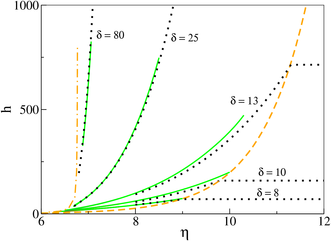
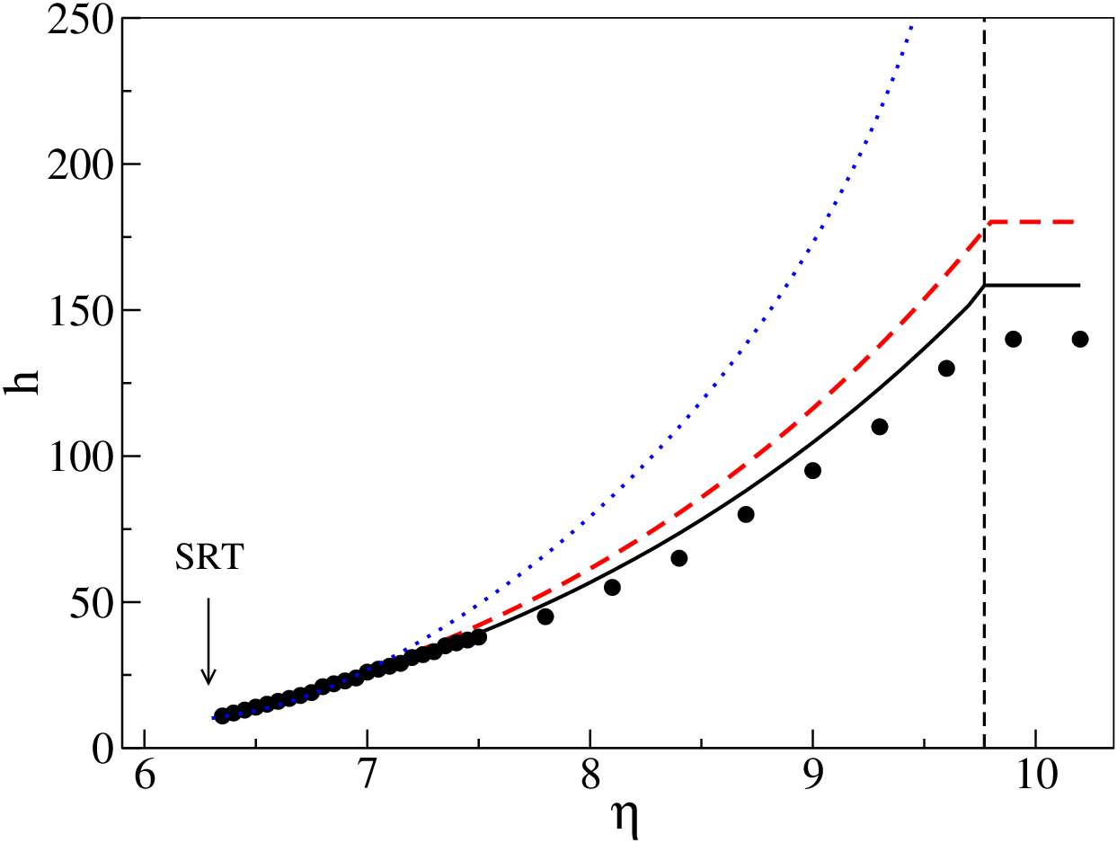
In Fig.7 we show the variation of stripe width vs. for different values of in the HWP, comparing the variational solution from Eqs.(21) and (23) using the approximation of Appendix D and the asymptotic approximation given by Eqs.(27) and (28). In Fig.8 we compare the equilibrium stripe width as a function of obtained within the different approximations used in this work for and with the MC simulations. Notice that the asymptotic approximation for the HWP given by Eqs.(27) and (28) shows a better agreement with the MC results than using the approximation (68) for the Fourier coefficients in the dipolar energy. This is because we adjusted the fitting parameter to optimize the agreement with the MC results at low values of . From Fig.7 we see that the discrepancy between both approximations becomes negligible in the large limit.
IV Discussion and conclusions
The main results of this work are summarized in Figs.1 and 6, which display the complete zero temperature phase diagram of the model defined by the Hamiltonian (1). Working upon reasonable assumptions for the ground states, like perfectly straight modulations in one dimension and Bloch domain walls, we analyzed minimum energy configurations combining a variational analysis with Monte Carlo results. We find four qualitatively different kinds of solutions: a planar ferromagnet for small anisotropies, and three types of perpendicular striped states: a canted state where the local magnetization has a finite in-plane component, a saturated state in which the in-plane component is restricted to the domain walls, and an Ising stripe state with sharp walls for large anisotropies.
The canted and staturated states give valuable information on the behaviour of the stripe width as the anisotropy and exchange parameters change, a still open and debated question[5, 9]. We find that stripe width variation is directly associated to the presence of finite width domain walls. For large enough values of the anisotropy the ground state of the system is always an Ising Striped state, no matter the value of the exchange coupling . In those states domain walls are sharp and the stripe width is completely independent of . It grows exponentially with the exchange coupling.
At the SRT the system always passes through a canted state as the anisotropy increases, although the range of values of where the canted angle is different from zero narrows as increases. The exchange to dipolar coupling ratio in fcc Fe based ultrathin films can be roughly estimated to be (considering a cubic bilayer of Fe/Cu(100), where[4] the exchange coupling , the lattice constant and[34] ). For the anisotropy interval for the canted phase is approximately . Although narrow, this suggests that the canted phase should be detectable close enough of the SRT, in systems like low temperature grown[35] Fe/Cu(100) or Fe/Ni/Cu films[5] (room temperature grown Fe/Cu(100) do not exhibit SRT[7], suggesting a rather large value of the microscopic anisotropy).
For stripe width variation appears always together with a varying canted angle. Close enough to the SRT domain walls present a sinusoidal shape in agreement with YG results, but as the anisotropy and the exchange increase, the wall profile changes to a hyperbolic tangent shape, as expected from micromagnetic calculations, while the magnetization inside the domains becomes fully saturated. For the ground state is given by the Saturated State, except very close to the SRT. A similar effect (i.e. a crossover between a sinusoidal and a saturated magnetization profile) has been observed in room temperature grown fcc Fe/Cu(100) ultrathin films, as the temperature decreases from , even though those systems do not present SRT[9].
In the Saturated state, the stripe width increase with is directly related to the wall width decrease through the relation . The wall width in turns is determined by the competition between exchange and anisotropy. Once the anisotropy is large enough that the wall width reaches the atomic limit, growth stops. One may wonder whether a similar mechanism could be behind the stripe width variation with temperature.
Besides its direct application to real systems, knowing the ground state of this system for arbitrary values of the exchange coupling is of fundamental importance to have a correct interpretation of Monte Carlo simulation results. Being one of the more powerful tools to analyze these kind of systems at the present (specially at finite temperatures), it is basically limited by finite size restrictions, which implies relatively small values of (the characteristic length of the problem grows exponentially with at low temperatures).
V Acknowledgments
We thank N. Saratz for advise about experimental results on ultrathin magnetic films. This work was partially supported by grants from CONICET, FONCyT grant PICT-2005 33305 , SeCyT-Universidad Nacional de Córdoba (Argentina), CNPq and CAPES (Brazil), and ICTP grant NET-61 (Italy).
Appendix A Yafet & Gyorgy Approximation
We briefly review in this appendix the derivation of the main results of YG approximation[13].
A.1 Energy per spin (Eq.(3))
The expression for the exchange and anisotropy energies per spin from Eq.(1) in terms of the one dimensional magnetization profile is straightforward:
| (34) |
The dipolar energy per spin can be expressed as , where is the self-interaction energy (i.e., the sum over of the interaction energy between spins belonging to the same line at ) and is the interaction energy between all different pairs of lines. The self interaction term is given by[13]
| (35) |
with
| (36) |
where is the Riemann Zeta function. The interaction term can be expressed as
| (37) |
where the sum in the above expression is taken over all values of such that . The interaction energy between two lines located at and is given by
| (38) |
where
| (39) |
| (40) |
In the limit the sums in Eqs.(39) and (40) can be evaluated using a continuum aproximation[13] giving and . For the error in this approximation is smaller than . For they can be evaluated numerically giving and . Then, Eq.(38) can be written as
| (41) | |||||
where and . Finally
| (42) | |||||
A.2 Variational equations for a striped magnetization profile with sinusoidal wall (SWP) in the continuum limit
In the continuum limit and () Eq.(14) can be written as
| (43) |
where and the functions are given in Eq.(10). From Eqs.(15) the Fourier cofficients in this limit are given by[13]
| (44) |
and[13]
| (45) |
| (46) |
| (47) |
Assuming a smooth profile inside the walls the exchange term in Eq.(43) can be approached by
| (48) |
Taking in the region inside a wall and replacing the summation in Eq.(48) by an integral we have that
| (49) |
| (50) |
where . Minimizing Eq.(50) respect to the variational parameters we get
| (51) | |||||
| (52) |
| (53) |
Notice that The fully saturated state is never a solution of the above equations, except in the limit (or ), which corresponds to . On the other hand, the planar ferromagnetic state (), is always solution of the above equations. For , the variational equations reduce to Eqs(17).
Close to the SRT (i.e., the transition between a state with and one with ) we can assume and therefore . Replacing into Eqs.(51)-(53) they become
| (54) | |||||
| (55) |
independent of , while Eq.(53) becomes identically zero in the limit (SRT). Replacing Eq.(54) into Eq.(55) we find
| (56) |
Both and the expression between square brackets in Eq.(56) are monotonously decreasing functions of[13] . Since the maximum allowed value is (which corresponds to . i.e., pure sinusoidal profile), the minimum value of for which a domain solution exists corresponds to . Using that[13] and we have
| (57) |
From Eq.(54) this corresponds to or . Replacing these values into Eq.(18) we see that in the limit we have that . Also from Eq.(50) we see that in this limit the planar ferromagnetic and the domain solutions become degenerated. Hence, this point corresponds to the SRT and the SRT line in the space is given by Eq.(19).
Appendix B Exact energy evaluation for a striped magnetization profile with sinusoidal wall (SWP) in a lattice
It is easier to carry out this calculation by considering a profile whose wall starts at , i. e.
| (58) |
where and . The profile Eq.(15) is related to the previous one by . The profile (58) can be expanded as
| (59) |
so the coefficients of the expansion (7) are given by
| (60) |
where stands for the real part of . The coefficients are given by
| (61) |
The summations in Eq.(61) can be carry out explicitly obtaining
| (62) |
where
| (63) |
with and
| (64) | |||||
The dipolar energy can then be evaluated from Eqs.(9) and (10). The anisotropy energy can be easily calculated and gives
| (65) |
The exchange and correction terms in Eq.(14) can be expressed as
| (66) |
| (67) | |||||
The summations in the above equations involve a finite number of terms that can be computed explicitly.
Appendix C Zero Temperature Monte Carlo Technique for striped domain patterns
In order to check the different striped profiles used to minimize the energy of the system, we implemented a simulated annealing protocol, based on Metropolis dynamics. The temperature was decreased down to zero at a constant rate , where the time is measured in Monte Carlo Steps. All the simulations are made starting from a planar ferromagnetic state with and . Every simulation is repeated times using a different sequence of random numbers, to check for possible trapping in local minima. Since we are considering only periodic straight domains with Bloch walls, the problem is basically one dimensional and we can restrict the search to a one dimensional pattern over the direction fixing and imposing periodic boundary conditions (PBC) in the direction. We also use PBC in the direction. In other words, we simulated a a lattice with with and PBC, which are implemented by means of the Ewald sums technique. For every set of values of we check the results for different values of in order to avoid artificial frustration. We also performed some comparisons with MC results in a square lattice; the results were indistinguishable. This ansatz allows us to obtain MC results for values of up to (for which the maximum equilibrium value is ).
Appendix D Fourier coefficients for the Hyperbolic Tangent wall Profile (HWP)
The function is very well approximated by
| (68) |
Then the Fourier coefficients for the profile Eq.(20) can be expressed as , where
| (69) |
and
| (70) |
where . Both integrals can be solved analytically, leading to rather long expressions that can be handled with symbolic manipulation programs.
References
- [1] R. Allenspach, M. Stamponi, and A. Bischof, Phys. Rev. Lett. 65, 3344 (1990).
- [2] A. Vaterlaus, C. Stamm, U. Maier, M. G. Pini, P. Politi, and D. Pescia, Phys. Rev. Lett. 84, 2247 (2000).
- [3] O. Portmann, A. Vaterlaus, and D. Pescia, Nature 422, 701 (2003).
- [4] Y. Wu, C. Won, A. Scholl, A. Doran, H. Zhao, X. Jin, and Z. Qiu, Physical Review Letters 93, 117205 (2004).
- [5] C. Won, Y. Wu, J. Choi, W. Kim, A. Scholl, A. Doran, T. Owens, J. Wu, X. Jin, H. Zhao, et al., Phys. Rev. B 71, 224429 (2005).
- [6] J. Choi, J. Wu, C. Won, Y. Z. Wu, A. Scholl, A. Doran, T. Owens, and Z. Q. Qiu, Phys. Rev. Lett. 98, 207205 (2007).
- [7] O. Portmann, A. Vaterlaus, and D. Pescia, Phys. Rev. Lett. 96, 047212 (2006).
- [8] O. Portmann, Micromagnetism in the Ultrathin Limit (Logos Verlag, 2006).
- [9] A. Vindigni, N. Saratz, O. Portmann, D. Pescia, and P. Politi, Phys. Rev. B 77, 092414 (2008).
- [10] M. Coisson, F. Celegato, E. Olivetti, P. Tiberto, and M. Baicco, J. Appl. Phys. 104, 033902 (2008).
- [11] N. Abu-Libdeh and D. Venus, arXiv:0905.2339v1 (2009).
- [12] T. Garel and S. Doniach, Phys. Rev. B 26, 325 (1982).
- [13] Y. Yafet and E. M. Gyorgy, Phys. Rev. B 38, 9145 (1988).
- [14] R. Czech and J. Villain, J. Phys. : Condensed Matter 1, 619 (1989).
- [15] D. Pescia and V. L. Pokrovsky, Phys. Rev. Lett. 65, 2599 (1990).
- [16] A. Kashuba and V. L. Pokrovsky, Phys. Rev. B. 48, 10335 (1993).
- [17] A. Abanov, V. Kalatsky, V. L. Pokrovsky, and W. M. Saslow, Phys. Rev. B 51, 1023 (1995).
- [18] P. Politi, Comments Cond. Matter Phys. 18, 191 (1998).
- [19] A. D. Stoycheva and S. J. Singer, Phys. Rev. E 64, 016118 (2001).
- [20] D. G. Barci and D. A. Stariolo, Physical Review Letters 98, 200604 (2007).
- [21] K. De’Bell, A. B. MacIsaac, and J. P. Whitehead, Rev. Mod. Phys. 72, 225 (2000).
- [22] S. A. Cannas, D. A. Stariolo, and F. A. Tamarit, Phys. Rev. B 69, 092409 (2004).
- [23] S. A. Cannas, M. Michelon, D. A. Stariolo, and F. A. Tamarit, Phys. Rev. B 73, 184425 (2006).
- [24] E. Rastelli, S. Regina, and A. Tassi, Phys. Rev. B 73, 144418 (2006).
- [25] A. Giuliani, J. L. Lebowitz, and E. H. Lieb, Phys, Rev. B 74, 064420 (2006).
- [26] S. A. Pighín and S. A. Cannas, Phys. Rev. B 75, 224433 (2007).
- [27] L. Nicolao and D. A. Stariolo, Phys. Rev. B . 76, 054453 (2007).
- [28] S. A. Cannas, M. Michelon, D. A. Stariolo, and F. A. Tamarit, Phys. Rev. E 78, 051602 (2008).
- [29] M. Carubelli, O. V. Billoni, S. A. Pighín, S. A. Cannas, D. A. Stariolo, and F. A. Tamarit, Phys. Rev. B 77, 134417 (2008).
- [30] J. P. Whitehead, A. B. MacIsaac, and K. De’Bell, Phys. Rev. B 77, 174415 (2008).
- [31] C. A. F. Vaz, J. A. C. Bland, and G. Lauhoff, Rep. Prog. Phys. 71, 056501 (2008).
- [32] G. Bertotti, Hysteresis in Magnetism (Academic Press, 1998).
- [33] I. S. Gradshteyn and I. M. Ryzhik, Table of Integrals, Series and Products (Academic Press, 1994), 5th ed.
- [34] J. H. Dunn, D. Arvanitis, and N. Mårtensson, Phys. Rev. B 54, R11157 (1996).
- [35] A. Enders, D. Peterka, D. Repetto, N. Lin, A. Dmitriev, and K. Kern, Phys. Rev. Lett. 90, 217203 (2003).