Galaxy-Scale Strong Lensing Tests of Gravity and Geometric Cosmology:
Constraints and Systematic Limitations
Alternate Affiliation: Based on observations made with the
NASA/ESA
Hubble Space Telescope, obtained
at the Space Telescope Science Institute, which is operated
by AURA, Inc., under NASA contract NAS 5-26555.
These observations are associated with programs No. 10174, No. 10494,
No. 10587, No. 10798, and No. 10886.
Abstract
Galaxy-scale strong gravitational lenses with measured stellar velocity dispersions allow a test of the weak-field metric on kiloparsec scales and a geometric measurement of the cosmological distance–redshift relation, provided that the mass-dynamical structure of the lensing galaxies can be independently constrained to a sufficient degree. We combine data on 53 galaxy-scale strong lenses from the Sloan Lens ACS Survey with a well-motivated fiducial set of lens-galaxy parameters to find (1) a constraint on the post-Newtonian parameter , and (2) a determination of under the assumption of a flat universe. These constraints assume that the underlying observations and priors are free of systematic error. We evaluate the sensitivity of these results to systematic uncertainties in (1) total mass-profile shape, (2) velocity anisotropy, (3) light-profile shape, and (4) stellar velocity dispersion. Based on these sensitivities, we conclude that while such strong-lens samples can in principle provide an important tool for testing general relativity and cosmology, they are unlikely to yield precision measurements of and unless the properties of the lensing galaxies are independently constrained with substantially greater accuracy than at present.
Subject headings
cosmological parameters — gravitational lensing — relativityI. Introduction
Einstein’s theory of general relativity (GR) has been an extremely successful description of gravity. It has passed all current experimental tests, most famously Eddington’s measurement of light deflection during the solar eclipse of 1919 [16]; observation of the gravitational redshift by Pound & Rebka [31]; the successful operation of the Global Positioning Satellites [1]; measurements of the Shapiro delay [36, 4]; and extensive studies of relativistic effects in binary radio pulsar systems, including verification of energy loss via gravitational waves as observed in the Hulse–Taylor pulsar [37]. Tests of gravity at ever higher precisions continue to be pursued through techniques such as lunar laser ranging, where the Earth-Moon separation is precisely measured as a function of time [41]. The parameterized post-Newtonian (PPN) framework [38] provides a systematic, quantitative way in which to formulate and interpret tests of gravity. The post-Newtonian parameter traditionally denoted by —a measure of the amount of spatial curvature per unit mass—is currently constrained to be [4] on solar-system length scales. Within the post-Newtonian parameterization of GR, has no scale dependence, and thus constraints on deviations from on significantly larger length scales can provide further tests of the theory.
GR has had further success in its application to physical cosmology. From assumptions of homogeneity and isotropy, the evolution of the universe as a function of time can be predicted from the knowledge of the densities of its constituents. While it was initially assumed that the density of the universe was dominated by matter (including a significant component of non-baryonic “dark matter”), the discovery that the universe is expanding at an accelerating rate (as traced by type Ia supernovae) has forced a modification of this idea [32, 30]. It is now thought that the universe is filled with a “dark energy”, an unknown substance with negative pressure. The composition of the universe determines its evolutionary history through the FRW metric and the Friedmann equations, and the evolution history of the universe in turn sets the distance-redshift relation. Thus, measurements of the conversion from redshift to distance constrain the density of dark energy, which we denote simply by in this work (i.e., assuming an equation of state ).
This paper presents an analysis of the quantitative constraints that can be placed on GR as a theory of gravity and on the density of dark energy in the universe using the large and homogeneous set of strong gravitational lens galaxies observed by the Sloan Lens ACS (SLACS) Survey collaboration [6]. To date, research using the SLACS sample has been primarily focused on constraining the internal structure and dynamics of the SLACS lenses under the assumption of GR and a CDM cosmology [39, 27, 19, 28, e.g.]. However, with reasonable prior assumptions and independent measurements of the structure of early-type galaxies such as the SLACS lenses, the problem can be inverted and the sample used to constrain the parameters of GR and of the cosmology. The first avenue was explored for an initial sample of 15 SLACS lenses by Bolton et al. [7], who found the post-Newtonian parameter to be on kiloparsec scales by adopting priors on early-type galaxy structure taken from observations of the local universe. The second avenue, originally suggested in passing by Golse et al. [21], was examined at length by Grillo et al. [22], who discussed the use of the SLACS lensing systems as a means to determine cosmological parameters, finding that the “concordance” values of fell within their 99% confidence regions. In both cases, the general approach consists of using angular “Einstein radii” measured from imaging, in combination with spectroscopic redshifts and parameterized galaxy mass models, to predict an observable stellar velocity dispersion—which explicitly depends upon the parameter of interest, whether post-Newtonian or cosmological—and then comparing this predicted value with the velocity dispersion measured from spectroscopy. Alternatively, these techniques can be characterized as treating strong-lensing Einstein radii as “standard angles” calibrated by the stellar velocity dispersions of the lensing galaxies. (Also see Gavazzi et al. [18] for a related cosmological application.)
In this work we re-examine the constraints that can be set on both and using strong gravitational lensing by early-type galaxies, given the availability of the expanded SLACS sample presented by Bolton et al. [8]. Our final emphasis will not be as much on the most probable values for these parameters, but rather on the uncertainties due to systematic errors made in estimating the properties of the lensing galaxies. In Section II, we discuss the SLACS lens sample that is used in our analysis. The lensing formalism that we utilize is reviewed in Section III. Our determination of and for a fiducial set of lensing parameters is presented in Section IV, along with a brief discussion of the statistical analysis that was employed. Section V is devoted to an in-depth evaluation of the effects that systematic errors in the lens parameters have on the nominal values for and . Finally, in Section VI we summarize our findings and draw some conclusions on how to improve the accuracy of strong lensing results in the future.
II. SLACS Lens Sample
The post-Newtonian strong-lensing constraints published by Bolton et al. [7] were based on a sample of 15 strong galaxy-galaxy gravitational lenses from the SLACS Survey, which are described in Bolton et al. [6], Treu et al. [39], and Koopmans et al. [27]. The current work uses a more recent and larger sample of strong lenses from this same survey, which is described in detail by Bolton et al. [8]. These systems were all selected from within the spectroscopic database of the Sloan Digital Sky Survey (SDSS: York et al. 43) based upon the presence of two significantly different galaxy redshifts within a single spectrum, obtained with a 3′′-diameter fiber aperture. As a consequence of explicit lensing and other selection effects, the SLACS sample consists primarily of massive, early-type (i.e., elliptical and S0) galaxies lensing much fainter and more distant emission-line galaxies.
For the present work, the key observables in each system are the redshifts of the two components (foreground “lens” and background “source”), the stellar velocity dispersion of the lens galaxy, a power-law index representing the characteristic slope of the luminosity profile, and the angular Einstein radius of the strongly lensed image of the more distant galaxy. The first three of these quantities are measured from SDSS spectroscopy, while the last two are measured from high-resolution follow-up images obtained by the SLACS survey through the F814W (-band) filter with the Wide Field Channel of the Advanced Camera for Surveys (ACS) aboard the Hubble Space Telescope (HST). Note that mass and light models fitted to the HST data include a projected axis-ratio parameter, , to capture ellipticity. To connect these models to the axisymmetric approximation of the analytic Jeans equation-based framework introduced below, we use the interchange
| (1) |
which conserves the total mass or light within a given isodensity or isobrightness contour and is consistent with the Einstein-radius and effective-radius measurement conventions of Bolton et al. [8].
The 53 lenses considered in this work are those from Bolton et al. [8] that have single lens galaxies with early-type morphology, successful quantitative strong lens models (and hence measured Einstein radii), and sufficiently high signal-to-noise measurements of lens-galaxy stellar velocity dispersion. These lens galaxies have redshifts in the range 0.1–0.3, and given these relatively low redshifts (and hence modest look-back times), there is unlikely to be significant structural difference between the SLACS lens galaxies and the local-universe elliptical galaxies that we and Bolton et al. [7] use as a calibration sample.
III. Lensing Formalism
We start with the weak-field PPN form of the Schwarzschild metric
| (2) |
with , where is a parameter to be constrained, and for GR. For thin gravitational lenses, the “lens equation” which governs the deflection of light is then
| (3) |
where is the angular location of the source, and is the angular location of the image. The scaled, projected Newtonian potential is defined as
| (4) |
where is the traditional Newtonian potential and is the line-of-sight distance between the observer and the source, with at the lens. Here, is the distance to the source, is the distance to the lens, and is the distance between the lens and the source; all three are cosmological angular-diameter distances.
For a lens that is cylindrically symmetric around the line of sight, the Einstein ring radius is found by setting to yield
| (5) |
The Einstein radius provides the characteristic angle (or length) in gravitational lensing. The angular size of the Einstein radius corresponding to a point mass is given by
| (6) |
For more general cylindrically symmetric mass distributions with respect to the line-of-sight, this continues to hold with , the mass contained within a cylinder of radius equal to the Einstein radius. Rearranging terms, and noting that , we find:
| (7) |
a form which will prove useful. Regardless of the extent of the mass distribution, only the mass interior to the Einstein radius has a net effect on the deflection of the light in the circularly symmetric (or, more generally, homoeoidal [35]) case.
We will mainly consider a flat cosmology, where and thus . This means there is only one free cosmological parameter appearing in the distance-redshift relation. This restriction on the dimension of the parameter space yields a sharper constraint (see Section IV). The assumption of flatness is not an unreasonable one. Currently, independent measurements show [25], and the theoretical prediction of inflation is that [24].
In this flat case, the relation among the angular diameter distance between two objects () and their line-of-sight comoving distances is
| (8) |
where is the redshift. Then, the ratio of angular diameter distances which appears in our expression for the Einstein radius is simply
| (9) |
Since this is a ratio of two comoving distances, there is no dependence on the Hubble constant. Thus, this ratio depends only on the source and lens redshifts, which are measured, and the choice of .
One of the simplest models one can write down for an elliptical galaxy is a scale-free model based on power-law density profiles for the total mass density, , and luminosity density, ,
| (10) | |||||
| (11) |
[26, see, e.g.,]. In general, the three-dimensional velocity dispersion tensor is not isotropic. The deviation can be characterized through the anisotropy parameter , defined as
| (12) |
where is the radial value. Having assumed spherical symmetry, , and we refer to this component as “tangential”. For the purpose of the current analysis it will suffice to assume that is independent of . This is the model used by by Bolton et al. [7] and discussed by Koopmans [26].
We define to be the spherical radial coordinate from the lens center and to be the cylindrical radius, i.e., perpendicular to the line of sight (defined to be along the -axis). So by definition .
A key ingredient in all the lensing measurements is the observed velocity dispersion, which is a projected, luminosity weighted average of the radially-dependent velocity dispersion profile of the lensing galaxy. In order to predict this value based on a set of galaxy parameters, we start with an expression, derived from the spherical Jeans equation, for , the radial velocity dispersion of the luminous matter (i.e., stars) [5]:
| (13) |
for the case where the velocity anisotropy parameter, , is a constant. Note that the use of Equation (13) is based on the assumption that the relationship between stellar number density and stellar luminosity density is spatially constant, an assumption unlikely to be violated appreciably within the effective radius of the early-type lens galaxies under consideration. Using the mass density profile in Equation (10), it is straightforward to show that the relation between the mass contained within a spherical radius and is
| (14) |
where we have defined the ratio of gamma functions
| (15) |
Therefore, after evaluating the integral in Equation (13) we find
| (16) |
where, following Koopmans [26], we have defined as a convenient combination of the power-law exponents.
Because all of the elliptical galaxy lenses in this study have been directly imaged with HST, we can measure their projected two-dimensional luminosity profiles. Following Bolton et al. [7], we directly fit point-spread function (PSF) convolved two-dimensional power-law ellipsoid images to HST F814W imaging data over a circle of radius 18 centered on the lens galaxies, adding 1 to the best-fit two-dimensional power-law index so as to account for a deprojection into three dimensions to obtain our adopted values for each system.
The velocity dispersions are measured from SDSS spectra. Each SDSS spectroscopic fiber subtends a circle of radius 15 on the sky, with atmospheric blurring adding an additional consideration. The actual aperture weighting function should thus be the convolution of the atmospheric seeing, represented by a Gaussian,
| (17) |
and the fiber aperture
| (18) |
where is the rectangle function as defined in Bracewell [10]. Then which has the form
| (19) |
where is a modified Bessel function of the first kind. We have evaluated Equation (19) numerically, and found that as long as , the convolution of the Gaussian and the top-hat will remain approximately Gaussian, where
| (20) |
and . Thus, we will later use
| (21) |
for the aperture weighting function in Equation (23). For each lens in our analysis, we take for the median value recorded by the spectroscopic guide cameras during the SDSS observations.
The actual velocity dispersion measured by the observations has been effectively luminosity-weighted along the line of sight and over the effective spectrometer aperture. This averaging can be expressed mathematically as:
| (22) |
where is the observational aperture weighting function defined above in Equation (21). In Equation (22) the factor takes into account how the radial and tangential components of the velocity dispersion tensor project along the line of sight. This integral expression for is analytic and, given the above definitions, it becomes
| (23) | |||||
where, again, is the ratio of gamma functions defined in Equation (15). Henceforth, we abbreviate as simply . One can immediately observe from Equation (23) that there are degeneracies among , and . The dependence upon enters this relation by way of the ratio .
IV. Determination of and
As mentioned previously, the general approach to generating a constraint is to compare the velocity dispersion from the SDSS observations, , with the velocity dispersion calculated from a galaxy model . By virtue of the analysis in the previous section, we have
| (24) |
where the semicolon separates the galaxy parameters and observables (, , , ) for which we have measured or adopted values from the global parameters (, ) which we are seeking to constrain.
We will generate the constraint by considering and its corresponding uncertainty to be a measurement with Gaussian errors such that the probability density for the observed value of given a “true” value of is
| (25) |
Statistical errors on , and the source and lens redshifts are negligible in comparison to the velocity dispersion errors and the intrinsic variation of the galaxy parameters and , and therefore we do not treat them explicitly.
We determine observational constraints for both and in a similar manner and thus the following discussion concerns our method of constraining a single parameter . In order to constrain we assume a standard flat cosmology with . In order to constrain , we assume that GR is correct and thus .
We are interested in calculating the probability of our observations having yielded a certain value of galaxy velocity dispersion, , given a particular assumed value of the parameter . We incorporate the dependence upon and by using the system-specific values determined from the HST imaging as discussed in Sections II and III, although in what follows we suppress and for notational convenience. Because we cannot independently measure and for individual lensing systems, we consider these values to be drawn from Gaussian distributions and with known mean and intrinsic scatter. For a given lens, the probability density of interest can be written as
| (26) |
Assuming a flat prior for over a range of interest, a universal value for in all systems, and statistical independence of the measurements of each system, the posterior probability for given the data is then proportional to the product over the individual probabilities:
| (27) | |||||
We illustrate this analysis by selecting a fiducial set of parameters. For and we choose a set of Gaussian distributions characterized by:
| (28) |
The cited 1- ranges in and are meant to indicate the intrinsic spreads in these quantities rather than uncertainties in the mean values. The mean of is fiducially taken to be simply 2.00, the slope of a singular isothermal sphere. This is the same value as adopted in the analysis of Grillo et al. [22]. This is also consistent with the value of determined for the same sample of SLACS lenses by Koopmans et al. [28] via an ensemble aperture-mass analysis, which is independent of any dynamical data or modeling and hence does not introduce circularity into our logic in proceeding to constraints on and . The scatter in and the distribution for are the same as used in Bolton et al. [7], and are taken to describe the distribution of mass-dynamical properties of the well-studied sample of nearby elliptical galaxies from Gerhard et al. [20]. Koopmans et al. [28] present a significantly higher value for the intrinsic scatter in , but argue that this value should be regarded as an upper limit given the likelihood of unmodeled systematic effects. For comparison with these adopted values of and , our measured values of have a mean of and a standard deviation .
Performing the analysis discussed above for , we find the resulting posterior probability density shown in Figure 1. A fit to a Gaussian gives (1 confidence). The result is consistent with and GR. Compared to the previous [7] result, , the statistical errors are reduced by a factor of as a result of the increase in the number of lensing systems considered (15 vs. 53). However, as we discuss in the next section, the systematic errors may be comparable to, or even dominate over, these statistical uncertainties, thereby preventing a large improvement in the precision of simply by increasing the sample size of gravitational lens systems.
We now set and establish a constraint on . Because the calculation, and in particular the ratio contained in Equation (23), is not very sensitive (at more than the level) to cosmological parameters, we restrict our attention to flat universes with . The resulting posterior probability density for is shown in Figure 2. The peak occurs at and the distribution has a best-fit Gaussian width (1 ) of . is clearly excluded. This constraint is consistent with the results from the cosmic microwave background, galaxy clusters, and type Ia supernovae. The recent WMAP5 data in combination with type Ia supernovae and baryon acoustic oscillations indicate and is also consistent with our assumption of a flat universe, giving the constraint [25].
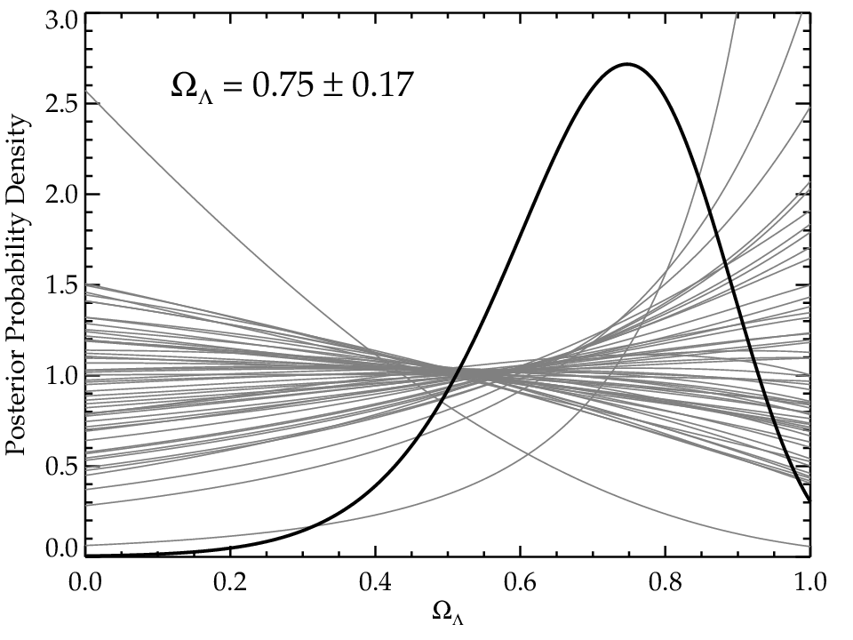

One can see from Figure 2 that none of the individual posterior probability density function (PDF) curves peak: all are either strictly increasing or decreasing. This bimodality occurs because of the relative insensitivity of to . A quick test shows that a reduction of the errors on by a factor of would induce a few of the flatter likelihood curves to peak. However, for most systems, there is no value of such that , which leads to the monotonic likelihood curves.
One may also observe that the posterior PDF curves for two of the systems rise or fall more sharply than the others. These two lens systems (J0252+0039 and J0737+3216) are among the high end of the SLACS sample in terms of lens redshift () but appear to be otherwise unremarkable. Neither lens strongly influences the final result: removing one or the other system shifts the peak posterior probability for by about three-quarters of a standard deviation, and removing both leaves the peak of the posterior probability approximately unchanged.
To illustrate the dependence of the ratio to the cosmological parameter , we show in Figure 3 the ratio as a function of the assumed value of for the 53 SLACS lenses. The curves are all normalized so that they yield a ratio of unity for a nominal value of . We see clearly from the curves in Figure 3 that the ratio of distances typically varies by and rarely by more than . The fractional statistical error in the inferred distance ratios for each system will be roughly 10–15%, or twice the fractional error in the measured velocity dispersion ( ; see Equation (23)). Therefore a determination of from an individual lens system can only be made at a “less-than-one-sigma” level. As previously noted by Grillo et al. [22], many lenses are required to obtain a statistically significant determination of .
V. The Effect of Systematics
Figure 1 shows the posterior PDF for the post-Newtonian parameter using fiducial values for the lens model parameters: , , and (see Equation (28)), the measured slopes of the light profiles, , and the values of the measured velocity dispersions, . The figure provides a clear estimate of the statistical uncertainty in , such that ( confidence). Similarly, Figure 2 shows the posterior PDF for the parameter using the same fiducial values for the lens model parameters as described here for determining , which yields a value for and its statistical uncertainty, .
However, each of the six lens parameters discussed above is susceptible to systematic error in either the adopted mean values ( and ), the assumed intrinsic widths ( and ), or in the directly measured parameters ( and ). It is therefore of crucial importance to test the sensitivity of our results for and to systematic shifts in the parameters associated with the lensing galaxies and to judge whether these sensitivities pose immediate and fundamental limitations to the precision of our constraints. To this end, we map out the dependence of the peak value of and (e.g., from results that are analogous to those shown in Figures 1 and 2) on the lens parameters. In particular, we vary over the range and over the range . We explore the effect of the assumed intrinsic widths by varying over the range and over the range . Next we shift all the measured values of dispersion velocity, by a multiplicative factor, , taken between 0.95 and 1.05, as well as all the measured slopes of the light distribution, , by an additive amount ranging from to 0.10. As we vary each of the these parameters in turn, the other parameters are held fixed at their fiducial values.

The results for the sensitivity of to systematic variations in the six lens parameters are shown in Figure 4. In each of the six panels the center of the plot is located at and at the fiducial value of the lens parameter being varied: , , , , , and , respectively. The values of the slopes of these curves (at the fiducial point) are summarized in Table 1. The analogously determined sensitivity of to systematic variations in the six lens parameters is shown in Figure 5, with the corresponding slopes also given in Table 1. The results are closely related to those for , except that they are typically a factor of 3 times larger in the case of than for . This is due to the fact that matching the model (as defined in Equation 23) to the measured is much more sensitively dependent on than it is on . Roughly speaking, is about three times more difficult to determine precisely than using strong lensing.
In general, one can see from Figures 4 and 5 and Table 1 that constraints on and are quite sensitive to small systematic shifts in the adopted lens-galaxy parameters. For example, a shift in the mean value of the slope of the mass profile of 0.04 in leads to a shift in of , a change that is nearly twice the statistical uncertainty associated with our measurement. Such a departure of from the value of 2.00, which amounts to just one-half of the adopted intrinsic scatter, is entirely plausible given the variation in this quantity as deduced from independent analyses and data sets (e.g., Gerhard et al. 20, Rusin et al. 34, Rusin & Kochanek 33, Bolton et al. 9, Koopmans et al. 28). More crucially, this same shift in would produce a change in of 0.29, a nearly fatal degradation of our constraint on this cosmological parameter. Shifts of comparable magnitude in and would be caused by a systematic error of 2.5% in the measured velocity dispersions, (i.e., ) which is well within the range of uncertainty due to possible mismatch between the stellar populations of the lens galaxies and the stellar spectrum template set used for the measurement of .
Though the effects are a bit less dramatic, similar statements hold for the sensitivity of the and results to the adopted intrinsic mass-slope scatter , the mean velocity anisotropy , and the systematic uncertainty in the light-profile slope . With respect to the last quantity, we note that although the power-law luminosity profile model that we have adopted could be improved upon with a different choice such as deVaucouleurs or Sérsic, the best-fit models from these classes still show significant departures from the HST imaging data. Thus the sensitivity of and constraints to systematic errors in the adopted luminosity profile is unlikely to improve much beyond the level presented here. Even massively parametric models for the luminosity profile such as the radial B-spline [6, 8] would be afflicted by systematic uncertainties related to ellipticity and deprojection. In addition, other currently unmodeled systematic effects such as selection effects [13, 29] and environmental overdensities [2, 40, 23], which appear to contribute only minorly to analyses of the structure of SLACS lenses under the assumption of and CDM, could have significant implications for the type of constraints considered in the current work.
| aaAll lens parameters are dimensionless and are defined in the text. | bbThe fiducial value at which the derivatives are evaluated. | ||
|---|---|---|---|
| 2.00 | 2.3 | 7.3 | |
| 0.18 | 0.64 | 2.3 | |
| 0.08 | 0.85 | 2.4 | |
| 0.13 | -0.03 | 0.06 | |
| 1.00 | -4.0 | -12 | |
| 0.00 | -0.9 | -2.9 |
From this analysis, we conclude that the systematics of the lens parameters must be controlled to a much tighter degree than currently appears possible before a more precise value of the post-Newtonian parameter can be determined, and before a meaningful independent determination of can be derived from strong gravitational lensing.
VI. Summary and Conclusions
In this work we have shown that, for a well-motivated set of fiducial lens-galaxy parameters, the current sample of 53 SLACS gravitational lensing galaxies can constrain either the post-Newtonian parameter (on kpc length scales), or the cosmological parameter . The statistical errors are such that the measurements provide an interesting level of precision (0.05 in and 0.17 in ). We have paid particular attention to quantifying the effects of systematic uncertainties in the lens parameters on the determination of and . These systematic errors are likely to be of equal or greater magnitude than the statistical uncertainties, so that the final result is largely limited by our imperfect knowledge of the galaxy parameters used in the analysis. In particular, the derivatives of both and with respect to several important lens parameters (enumerated in §5) have been calculated; these are displayed graphically in Figures 4 and 5 and tabulated in Table 1.
The larger lens sample we use as compared to that of Bolton et al. [7] has enabled us to reduce the statistical error on by a factor of 1.5 (from 0.07 to 0.05). However, since the uncertainty in due to the systematic errors in the lens parameters is likely to be at least as large as the statistical errors, simply increasing the lens sample will not improve the constraints on until the lens parameters are better understood.
Measurements of based on strong lensing involve different sets of assumptions than other experimental methods, and therefore could provide a useful independent estimate of this important cosmological parameter. However, our results show that in order for strong lensing by galaxies to become effective in determining , our independent knowledge of lens-galaxy mass-dynamical structure will have to improve by an order of magnitude.
Future observations and analysis have some prospect of improving this situation. High-resolution ground-based spectroscopy with large telescopes and good seeing can reduce both the statistical and systematic errors on the measured velocity dispersions (Czoske et al. 12, Barnabè et al. 3), and may indeed be able to provide a measurement of the average velocity anisotropy for some systems. A more detailed, spatially resolved dynamical analysis of nearby galaxies such as from the SAURON survey (Emsellem et al. 17, Cappellari et al. 11) could be used to derive more accurate prior distributions on lens-galaxy mass-model parameters, providing that the differing selection effects between SLACS and SAURON samples can be effectively controlled. Finally, system-by-system constraints on galaxy mass profiles using higher-order information contained in lensing data alone (e.g., Dye & Warren 15, Willis et al. 42, Dye et al. 14) could be used to remove some of the need for independent priors.
References
- [1] Ashby, N. 2002, Phys. Today, 55, 050000
- [2] Auger, M. W. 2008, MNRAS, 383, L40
- [3] Barnabè, M., Czoske, O., Koopmans, L. V. E., Treu, T., Bolton, A. S., & Gavazzi, R. 2009, MNRAS, 399, 21
- [4] Bertotti, B., Iess, L., & Tortora, P. 2003, Nature, 425, 374
- [5] Binney, J. 1980, MNRAS, 190, 873
- [6] Bolton, A. S., Burles, S., Koopmans, L. V. E., Treu, T., & Moustakas, L. A. 2006a, ApJ, 638, 703
- [7] Bolton, A. S., Rappaport, S., & Burles, S. 2006b, Phys. Rev. D, 74, 061501
- [8] Bolton, A. S., et al. 2008a, ApJ, 682, 964
- [9] —. 2008b, ApJ, 684, 248
- [10] Bracewell, R. N. 1986, The Fourier Transform and its Applications (New York: McGraw-Hill)
- [11] Cappellari, M., et al. 2006, MNRAS, 366, 1126
- [12] Czoske, O., Barnabè, M., Koopmans, L. V. E., Treu, T., & Bolton, A. S. 2008, MNRAS, 384, 987
- [13] Dobler, G., Keeton, C. R., Bolton, A. S., & Burles, S. 2008, ApJ, 685, 57
- [14] Dye, S., Evans, N. W., Belokurov, V., Warren, S. J., & Hewett, P. 2008, MNRAS, 388, 384
- [15] Dye, S., & Warren, S. J. 2005, ApJ, 623, 31
- [16] Dyson, F. W., Eddington, A. S., & Davidson, C. 1920, Phil. Trans. R. Soc., 220, 291
- [17] Emsellem, E., et al. 2004, MNRAS, 352, 721
- [18] Gavazzi, R., Treu, T., Koopmans, L. V. E., Bolton, A. S., Moustakas, L. A., Burles, S., & Marshall, P. J. 2008, ApJ, 677, 1046
- [19] Gavazzi, R., et al. 2007, ApJ, 667, 176
- [20] Gerhard, O., Kronawitter, A., Saglia, R. P., & Bender, R. 2001, AJ, 121, 1936
- [21] Golse, G., Kneib, J.-P., & Soucail, G. 2002, A&A, 387, 788
- [22] Grillo, C., Lombardi, M., & Bertin, G. 2008, A&A, 477, 397
- [23] Guimarães, A. C. C., & Sodré, L. J. 2009, arXiv:0904.4381
- [24] Guth, A. H. 1981, Phys. Rev. D, 23, 347
- [25] Komatsu, E., et al. 2009, ApJS, 180, 330
- [26] Koopmans, L. V. E. 2006, in EAS Publications Series, ed. G. A. Mamon, F. Combes, C. Deffayet, & B. Fort, Vol. 20, 161
- [27] Koopmans, L. V. E., Treu, T., Bolton, A. S., Burles, S., & Moustakas, L. A. 2006, ApJ, 649, 599
- [28] Koopmans, L. V. E., et al. 2009, ApJ, 703, L51
- [29] Mandelbaum, R., van de Ven, G., & Keeton, C. R. 2009, MNRAS, 398, 635
- [30] Perlmutter, S., et al. 1999, ApJ, 517, 565
- [31] Pound, R. V., & Rebka, G. A. 1960, Phys. Rev. Lett., 4, 337
- [32] Riess, A. G., et al. 1998, AJ, 116, 1009
- [33] Rusin, D., & Kochanek, C. S. 2005, ApJ, 623, 666
- [34] Rusin, D., Kochanek, C. S., & Keeton, C. R. 2003, ApJ, 595, 29
- [35] Schramm, T. 1990, in Lecture Notes in Physics, Vol. 360, Gravitational Lensing, ed. Y. Mellier, B. Fort, & G. Soucail (Berlin: Springer), 46
- [36] Shapiro, I. I. 1964, Phys. Rev. Lett., 13, 789
- [37] Taylor, J. H., Fowler, L. A., & McCulloch, P. M. 1979, Nature, 277, 437
- [38] Thorne, K. S., & Will, C. M. 1971, ApJ, 163, 595
- [39] Treu, T., Koopmans, L. V., Bolton, A. S., Burles, S., & Moustakas, L. A. 2006, ApJ, 640, 662
- [40] Treu, T., et al. 2009, ApJ, 690, 670
- [41] Williams, J. G., Turyshev, S. G., & Boggs, D. H. 2004, Phys. Rev. Lett., 93, 261101
- [42] Willis, J. P., Hewett, P. C., Warren, S. J., Dye, S., & Maddox, N. 2006, MNRAS, 369, 1521
- [43] York, D. G., et al. 2000, AJ, 120, 1579