1Introduction

WIS/10/09-JULY-DPP

APCTP Pre2009 - 010

Large- $N$ reduced models of supersymmetric

quiver, Chern-Simons gauge theories and ABJM

Masanori Hanada^a¹¹ 1 E-mail address : masanori.hanada@weizmann.ac.il, Lorenzo Mannelli^a²² 2 E-mail address : lorenzo.mannelli@weizmann.ac.il and Yoshinori Matsuo^b³³ 3 E-mail address : ymatsuo@apctp.org

^a Department of Particle Physics, Weizmann Institute of Science,
Rehovot 76100, Israel

^b Asia Pacific Center for Theoretical Physics,
Pohang, Gyeongbuk 790-784, Korea

Abstract

Using the Eguchi-Kawai equivalence, we provide regularizations of supersymmetric quiver and Chern-Simons gauge theories which leave the supersymmetries unbroken. This allow us to study many interesting theories on a computer. As examples we construct large- $N$ reduced models of supersymmetric QCD with flavor and the ABJM model of multiple M2 branes.

1 Introduction

Super Yang-Mills theories (SYM) have attracted much interests as leading candidates for physics beyond the standard model. To understand their nonperturbative aspects, one might expect lattice simulation to be useful as it happens in the usual non-supersymmetric gauge theories. However, it is generally difficult to realize SYM on lattices and consequently detailed numerical simulations have been performed only in lower (less than four) dimensions (see [1] for recent simulations of 4d SYM, and [2] for a review of lattice supersymmetry).

SYM’s are also important because it is expected to provide a nonperturbative formulation of superstring/M theory at large- $N$ [3, 4, 5, 6, 7]. In this context the relevant theories are SYM’s in lower dimensional spacetime. In particular, $(0+1)$ -dimensional theory can be analyzed on computer by using the non-lattice technique [8] (in this case lattice simulations are also possible [9]) and a part of these conjectures has been confirmed by Monte-Carlo simulations in the strong coupling regime [10, 11, 12]. Chern-Simons gauge theories are also relevant in the context of superstring/M theory. In fact recently supersymmetric Chern-Simons gauge theories in three dimensions have been proposed as a description of the theory of multiple M2-branes [13, 14]. Since these theories describe membranes in their strong coupling regimes, numerical simulations appear to be a very useful tool. Unfortunately it turns out to be a very difficult task to study either Chern-Simons or supersymmetry on a lattice.

At large- $N$ , it is possible to circumvent the lattice-SUSY problem by using the Eguchi-Kawai equivalence [15]. This construction guarantees that the large- $N$ gauge theories are equivalent to the lower dimensional matrix models if a certain condition is satisfied. Recently this equivalence has been used to formulate 4d ${\cal N}=4$ SYM compactified on $S^{3}$ [16].⁴⁴ 4 For other attempts that use the Eguchi-Kawai equivalence, see [17, 18, 19]. In this construction, the BMN matrix model [20] around a certain multi-fuzzy sphere solution is argued to be equivalent, using the Eguchi-Kawai reduction, to 4d ${\cal N}=4$ SYM. (For evidence supporting the validity of this formulation, see [21].) Given that the solution is BPS, it provides a regularization that preserve part of supersymmetry. Furthermore, given that one-dimensional system like the BMN model can be analyzed on computer, the previous formulation allows us to study 4d SYM using a Monte-Carlo simulation.

A natural question to ask is to which kind of theories it is possible to apply the Eguchi-Kawai equivalence. The generalization to 4d ${\cal N}=1$ pure SYM is quite straightforward, as discussed in [22], using the matrix model analyzed in [23]. However, introducing fundamental matter, as will be explained in § 3, turns out to be a difficult task⁵⁵ 5 As discussed in [24], large- $N$ gauge theories with a quark in the two-index antisymmetric representation can be regarded as the counterpart of the usual QCD, in the sense that this representation reduces to the fundamental representation when $N=3$ . For these models, Eguchi-Kawai reduction can easily applied. See e.g. [18]. . In this paper, we show that quiver and Chern-Simons gauge theories can be regularized using the techniques of [16]. More specifically, in § 3 we construct the supersymmetric $SU(N)\times SU(M)$ gauge theory with bifundamental matter. Then, by sending the coupling constant of the latter gauge group to zero, we obtain a global flavor symmetry from this gauge symmetry, and as a consequence, this quiver gauge theory becomes supersymmetric QCD. In this construction both $N_{c}=N$ and $N_{f}=MK$ ( $K$ is the number of bifundamental matters) must be infinite, but the ratio $N_{f}/N_{c}$ can be arbitrary. In § 4 we show that Chern-Simons theory, which is difficult to study on lattice, can also be formulated in terms of Eguchi-Kawai equivalence. For that purpose, we use a construction of the Chern-Simons theory using a generalization of Taylor’s T-duality prescription [26] which is discussed in [25]. Combining this results with the technique of [16] the Eguchi-Kawai formulation can be obtained straightforwardly. ⁶⁶ 6 While this work was in progress we have been informed that the same idea had been studied by Ishiki et al [27]. We thank G. Ishiki for the discussion. Furthermore combining the analysis for the quiver and Chern-Simons theories, we are able to construct the ABJM theory [14] from a matrix model.

This paper is organized as follows. In § 2 we review the basic ideas of the Eguchi-Kawai equivalence. First, in § 2.1, we explain the quenched Eguchi-Kawai model [28, 29]. Based on it, in § 2.2, we review the reduced model of SYM on $S^{3}$ [16]. In § 3 we generalize this technique to construct supersymmetric quiver gauge theories. In § 4 we formulate Chern-Simons theory in three dimensions along the line of [25]. Combining these results with the ones in § 3 we construct the Chern-Simons-matter theories which recently attracted much interest as the theory describing multiple M2-branes.

2 The basics of the Eguchi-Kawai reduction

In this section we review the Eguchi-Kawai equivalence [15]. In §2.1 we introduce the “quenched” version of the Eguchi-Kawai model [28, 29], which is relevant for our purpose. In § 2.2 we use this technique to formulate large- $N$ Yang-Mills on the three-sphere.

2.1 Quenched Eguchi-Kawai model

In the following we review the diagrammatic approach to the quenched Eguchi-Kawai model(QEK) [29]. The basic idea is that in the planar limit, Yang-Mills theory is equivalent to a matrix model around a suitable background. We will also consider QEK for compact space [16, 30]. In order to see clearly the difference between the compact and noncompact cases, we consider (analogously to [16]) the simplest example first, namely the correspondence between a zero-dimensional matrix model and a matrix quantum mechanics.

As a simple example, we consider a matrix quantum mechanics with a mass term,

\displaystyle S_{1d}=N\int dtTr\left(\frac{1}{2}(D_{t}X_{i})^{2}-\frac{1}{4}[X_{i},X_{j}]^{2}+\frac{m^{2}}{2}X_{i}^{2}\right),

(1)

where $X_{i}\ (i=1,2,\cdots,d)$ are $N\times N$ traceless Hermitian matrices. The covariant derivative $D_{t}$ is given by

\displaystyle D_{t}X_{i}=\partial_{t}X_{i}-i[A,X_{i}].

(2)

At large- $N$ , this model can be reproduced starting from the zero-dimensional model

\displaystyle S_{0d}=\frac{2\pi}{\Lambda}\cdot NTr\left(-\frac{1}{2}[Y,X_{i}]^{2}-\frac{1}{4}[X_{i},X_{j}]^{2}+\frac{m^{2}}{2}X_{i}^{2}\right),

(3)

where $Y$ and $X_{i}$ are $N\times N$ traceless Hermitian matrices. We embed the (regularized) translation generator into the matrix $Y$ ,

\displaystyle Y^{b.g.}=diag(p_{1},\cdots,p_{N}),\qquad p_{k}=\frac{\Lambda}{N}\left(k-\frac{N}{2}\right).

(4)

By expanding $Y$ around this background,

\displaystyle Y=Y^{b.g.}+A,

(5)

the Feynman rules of the one-dimensional theory, as we will see in the following, are reproduced at large- $N$ .

The action can be rewritten as

\displaystyle S_{0d}=\frac{2\pi}{\Lambda}\cdot N\Biggl\{\frac{1}{2}\sum_{i,j}\left|(p_{i}-p_{j})\left(X_{k}\right)_{ij}-i[A,X_{k}]_{ij}\right|^{2}+Tr\left(-\frac{1}{4}[X_{i},X_{j}]^{2}+\frac{m^{2}}{2}X_{i}^{2}\right)\Biggl\}.

(6)

We add to it the gauge-fixing and Faddeev-Popov terms

\displaystyle\frac{2\pi}{\Lambda}\cdot NTr\left(\frac{1}{2}[Y^{b.g.},A]^{2}-[Y^{b.g.},b][Y,c]\right).

(7)

Then, the planar diagrams are the same as the ones in the 1d theory up to a normalization factor. For example, a scalar two-loop planar diagram with quartic interaction (see Fig.1) is

	$\displaystyle\frac{d(d-1)}{2}\left(\frac{1}{2}\cdot\frac{2\pi N}{\Lambda}\right)\sum_{i,j,k=1}^{N}\frac{(\Lambda/2\pi N)}{(p_{i}-p_{k})^{2}+m^{2}}\frac{(\Lambda/2\pi N)}{(p_{j}-p_{k})^{2}+m^{2}}$				(8)
		$\displaystyle\simeq$	$\displaystyle\frac{d(d-1)}{4}\cdot\frac{2\pi}{\Lambda}\cdot N^{2}\int^{\Lambda/2}_{-\Lambda/2}\frac{dp}{2\pi}\int^{\Lambda/2}_{-\Lambda/2}\frac{dq}{2\pi}\frac{1}{(p^{2}+m^{2})(q^{2}+m^{2})}.$		(8)

The essence of this expression is that the adjoint action of the background matrix can be identified with the derivative and the matrix elements of the fluctuations can be identified with the Fourier modes in momentum space. The corresponding diagram in the 1d theory is

\displaystyle\frac{d(d-1)}{4}\cdot Vol\cdot N^{2}\int^{\Lambda/2}_{-\Lambda/2}\frac{dp}{2\pi}\int^{\Lambda/2}_{-\Lambda/2}\frac{dq}{2\pi}\frac{1}{(p^{2}+m^{2})(q^{2}+m^{2})},

(9)

where $Vol$ is volume of the spacetime. Hence by interpreting $\Lambda$ and $\Lambda/N$ to be UV and IR cutoffs, those diagrams agree up to the factor $\left(\frac{\Lambda}{2\pi}\right)\cdot Vol$ . The other planar diagrams also correspond up to the same factor.

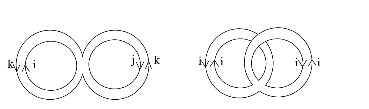
Refer to caption — Figure 1: Two-loop planar and nonplanar diagrams with quartic interaction vertex.

The nonplanar diagrams do not have such a correspondence, but in an appropriate limit they are negligible. In the 1d theory, by taking a planar limit they are suppressed by a factor $N^{-2}$ . In the reduced model, they are suppressed if IR cutoff $\Lambda/N$ goes to zero. To see this, let us calculate for example the two-loop nonplanar diagram in Fig.1. It reads

\displaystyle-\frac{d(d-1)}{4m^{4}}\frac{\Lambda}{2\pi},

(10)

which is suppressed by a factor $(\Lambda/N)^{2}$ compared with planar diagrams.

Therefore, by taking the limit

\displaystyle N\to\infty,\qquad\Lambda\to\infty,\qquad\frac{\Lambda}{N}\to 0

(11)

the 1d model on ${\mathbb{R}}$ is reproduced from the 0d model.

If one wants to obtain the theory on a circle, it is necessary to fix the IR cutoff while suppressing nonplanar diagrams. This can be achieved by taking the background to be

\displaystyle Y^{b.g.}=diag(p_{1},\cdots,p_{n_{1}})\otimes\textbf{1}_{n_{2}},\qquad p_{k}=\frac{\Lambda}{n_{1}}\left(k-\frac{n_{1}}{2}\right),\qquad N=n_{1}n_{2},

(12)

and taking $n_{1},n_{2}$ and $\Lambda$ to be infinity while fixing the IR cutoff $\Lambda/n_{1}$ [16].⁷⁷ 7 Another reason to consider the $n_{2}\to\infty$ limit is the following, if we take $n_{2}=1$ and quench the background, no zero-mode appears. This is not a problem when we take the noncompact limit, because the IR cutoff goes to zero. On the other hand, when we consider a compact space, the absence of the zero-mode destroys the Eguchi-Kawai equivalence. It turns out that by taking the $n_{2}\to\infty$ limit, zero-modes are taken into account in an appropriate manner.

It turns out that in this setup the background is not stable. So, to make the expansion meaningful, we have to “quench” the eigenvalues of $Y$ , i.e. we have to fix the background by hand. This is the reason for the name “quenched” Eguchi-Kawai model.

2.2 Eguchi-Kawai construction of Yang-Mills on $S^{3}$

Next let us construct the Yang-Mills theory on the three-sphere by using the Eguchi-Kawai equivalence. The essence of QEK is to find a background whose adjoint action can be identified with the spacetime derivative. So, the strategy is to find a set of three matrices whose adjoint action can be identified with the derivative on $S^{3}$ . Such matrices were found in [31, 16]. In the following we will show the derivation in a heuristic way.

2.2.1 YM on $S^{3}$

In this section, we express the action of Yang-Mills theory on $\mathbb{R}\times S^{3}$ in a form convenient for our purpose [16]. The radius of the sphere is taken to be $2/\mu$ . The action of $U(N)$ SYM is given by

\displaystyle S=-\frac{N}{\lambda_{4d}}\int dt\int_{S^{3}}d^{3}x\sqrt{-g(x)}Tr\frac{1}{4}F_{\mu\nu}^{2},

(13)

where $\lambda_{4d}$ is the ’t Hooft coupling constant, $g_{\mu\nu}(x)$ is the metric and $g(x)$ is its determinant. The field strength is

\displaystyle F_{\mu\nu}=\partial_{\mu}A_{\mu}-\partial_{\nu}A_{\mu}-i[A_{\mu},A_{\nu}].

(14)

The Greek indices $\mu$ , $\nu$ refer to the Einstein frame and the Latin indices to the local Lorentz frame.

The sphere part of this geometry has the group structure of $SU(2)$ . Given this group structure, there exists a right-invariant 1-form $dgg^{-1}$ and its dual Killing vectors ${\cal L}_{i}$ , satisfying the commutation relation

\displaystyle[{\cal L}_{i},{\cal L}_{j}]=i\epsilon_{ijk}{\cal L}_{k}.

(15)

Using the coordinates $(\theta,\psi,\varphi)$ defined by $g=e^{-i\varphi\sigma_{3}/2}e^{-i\theta\sigma_{2}/2}e^{-i\psi\sigma_{3}/2}$ , the vielbein $E^{i}$ can be expressed as

$\displaystyle E^{1}$	$\displaystyle=$	$\displaystyle\frac{1}{\mu}\left(-\sin\varphi d\theta+\sin\theta\cos\varphi d\psi\right),$	(16)
$\displaystyle E^{2}$	$\displaystyle=$	$\displaystyle\frac{1}{\mu}\left(\cos\varphi d\theta+\sin\theta\sin\varphi d\psi\right),$	(17)
$\displaystyle E^{3}$	$\displaystyle=$	$\displaystyle\frac{1}{\mu}\left(d\varphi+\cos\theta d\psi\right).$	(18)

In these coordinates the metric is given by

ds^{2}=\frac{1}{\mu^{2}}\left[d\theta^{2}+\sin^{2}\theta\,d\varphi^{2}+\left(d\psi+\cos\theta\,d\varphi\right)^{2}\right].

(19)

The spin connection $\omega_{abc}$ can be read off from the Maurer-Cartan equation,

	$\displaystyle dE^{i}-\omega^{i}_{\ jk}E^{j}\wedge E^{k}$	$\displaystyle=$	$\displaystyle 0,$		(20)
	$\displaystyle\omega_{ijk}$	$\displaystyle=$	$\displaystyle\frac{\mu}{2}\epsilon_{ijk}.$		(21)

and the Killing vectors are given by

\displaystyle{\cal L}_{i}=-\frac{i}{\mu}E_{i}^{M}\partial_{M},

(22)

where

$\displaystyle{\cal L}_{1}$	$\displaystyle=$	$\displaystyle-i\left(-\sin\varphi\partial_{\theta}-\cot\theta\cos\varphi\partial_{\varphi}+\frac{\cos\varphi}{\sin\theta}\partial_{\psi}\right),$
$\displaystyle{\cal L}_{2}$	$\displaystyle=$	$\displaystyle-i\left(\cos\varphi\partial_{\theta}-\cot\theta\sin\varphi\partial_{\varphi}+\frac{\sin\varphi}{\sin\theta}\partial_{\psi}\right),$
$\displaystyle{\cal L}_{3}$	$\displaystyle=$	$\displaystyle-i\partial_{\varphi}.$	(23)

The Killing vectors represent a complete basis for the tangent space on $S^{3}$ . Furthermore given that the vielbeins are defined everywhere on $S^{3}$ , the indices $i$ can be used as a label for the vector fields and 1-forms.⁸⁸ 8 This property is necessary in order to identify this index with the one in the matrix model [32].

By using the Killing vectors ${\cal L}_{i}$ , the action can be rewritten as [16]

$\displaystyle S$	$\displaystyle=$	$\displaystyle\left(\frac{2}{\mu}\right)^{3}\frac{N}{\lambda_{4d}}\int dt\int d\Omega_{3}Tr\Biggl(\frac{1}{2}\left(D_{t}A_{i}-\mu{\cal L}_{i}A_{t}\right)^{2}$	(24)
		$\displaystyle\qquad\qquad+\frac{\mu^{2}}{4}({\cal L}_{i}A_{j}-{\cal L}_{j}A_{i})^{2}-\frac{\mu}{2}({\cal L}_{i}A_{j}-{\cal L}_{j}A_{i})[A_{i},A_{j}]+\frac{1}{4}[A_{i},A_{j}]^{2}$
		$\displaystyle\qquad\qquad-\frac{\mu^{2}}{2}A_{i}^{2}+i\mu\epsilon^{ijk}A_{i}A_{j}A_{k}-i\mu^{2}\epsilon^{ijk}A_{i}({\cal L}_{j}A_{k})\Biggl),$

where $A_{i}$ is defined in such a way that the 1-form of the gauge field on $S^{3}$ take the form $A=A_{i}E^{i}$ , and $d\Omega_{3}$ is the volume form of the unit three-sphere.

2.2.2 Eguchi-Kawai reduction

To construct matrices which represent derivatives on $S^{3}$ in a coordinate-independent way, it is useful to use the $SU(2)$ group structure of $S^{3}$ . The Killing vectors (23) act on functions on $S^{3}\simeq SU(2)$ , whose irreducible decomposition is⁹⁹ 9 In general, for a compact Lie group $G$ , a space of functions on $G$ is decomposed as $\displaystyle{\cal C}^{\infty}(G)=\bigoplus_{r}\left(\underset{d_{r}-{\rm times}}{\underbrace{V_{r}\oplus\cdots\oplus V_{r}}}\right),$ (25) where $r$ runs over all the irreducible representations, $V_{r}$ is a representation space and $d_{r}$ is its dimension.

\displaystyle{\cal C}^{\infty}(SU(2))=\bigoplus_{J=0,1/2,1,\cdots}\left(\underset{(2J+1)\text{-times}}{\underbrace{V_{J}\oplus\cdots\oplus V_{J}}}\right),

(26)

where $V_{J}$ is the space that the spin $J$ representation acts on.

In order to realize this representation as the adjoint action of the background matrices, we first embed the $SU(2)$ generators into $N\times N$ matrices. We then introduce the matrices $L_{i}$ which satisfy the commutation relation of the $SU(2)$ generators,

[L_{i},L_{j}]=i\epsilon_{ijk}L_{k}.

(27)

Since these matrices cannot be diagonalized simultaneously, we embed them in the following block diagonal form;

\displaystyle L_{i}=\left(\begin{array}[]{ccccc}\ddots&&&&\\ &L_{i}^{[j_{s-1/2}]}&&&\\ &&L_{i}^{[j_{s}]}&&\\ &&&L_{i}^{[j_{s+1/2}]}&\\ &&&&\ddots\end{array}\right),

where $L_{i}^{[j_{s}]}$ is a $(2j_{s}+1)\times(2j_{s}+1)$ matrix which acts on the spin $j_{s}$ representation. The size of the matrix $N$ is

\displaystyle N=\sum_{s}(2j_{s}+1).

(34)

We introduce a regularization by restricting the representation space to a limited number of $j_{s}$ . Furthermore we take the integer $s$ satisfying

\displaystyle-\frac{T}{2}\leq s\leq\frac{T}{2},

(35)

where $T$ is an even integer. We introduce another integer $P\gg T$ and take $j_{s}$ to be

\displaystyle j_{s}=\frac{P+s}{2}.

(36)

The large $N$ limit is taken in the following way

\displaystyle P\to\infty,\qquad T\to\infty,\qquad N\to\infty.

(37)

To see how this prescription works, let us consider the $(j,j^{\prime})$ -block, to which $L^{[j]}$ acts from left and $L^{[j^{\prime}]}$ acts from the right. A Basis for this block is symbolically written as

\displaystyle|j,m\rangle\langle j^{\prime},m^{\prime}|.

(38)

It can be decomposed into spin $|j-j^{\prime}|,\cdots,j+j^{\prime}$ representations. Let’s count the number of representations of each spin.

Spin	0 :	$T+1$ , because it appears only when $j=j^{\prime}\geq 0$ .
Spin	1/2 :	$2T$ , because it appears when $j=j^{\prime}\pm 1/2$ .
Spin	1 :	$(T+1)+2(T-1)=3T-1$ , because it appears when $j=j^{\prime}\geq 1$ and $j=j^{\prime}\pm 1$ .
Spin	$J\in{\mathbb{Z}}$ :	$(T+1)+\sum_{l=1}^{J}2(T+1-2l)=(2J+1)T+1-2J^{2}$ .

As long as $T\gg J$ , we can approximate this expression as

\displaystyle({\rm number\ of\ spin\ }J)\simeq(2J+1)T.

(39)

Therefore the representation space, or equivalently the variables appearing in the matrix model, can be regarded as a set of $T$ copies of the space of functions on $S^{3}$ . As $J$ increase the number of copies decreases. In this sense $T$ plays a role of a momentum cutoff.

In this way matrix elements can be identified with the functions on $S^{3}$ , or in other words the propagators in the Feynman diagram agrees. However it is not apparent if this identification is consistent with the multiplication of the fields. (This is necessary in order for the interaction vertices to agree.) In [16] it has been shown that

\displaystyle\frac{T}{P}\to 0

(40)

is a sufficient condition for the compatibility with the multiplication.¹⁰¹⁰ 10 Given that this condition force us to use very large matrix in a computer simulation, it would be nice if it could be relaxed. However this seems to be impossible because the eigenvalue distribution is not uniform without imposing $T/P\to 0$ , while the eigenvalues should be distributed uniformly in order for the quenched Eguchi-Kawai equivalence to work. One possible solution is to make the density uniform by putting fuzzy spheres with the same radii on top of each other and tune the number of copies to be proportional to the spin. We thank G. Ishiki for stimulating discussion on this point.

By using these matrices we can relate a matrix model to a gauge theory on $S^{3}$ , given by the action (24). In order to do that, we consider the bosonic matrix quantum mechanics

\displaystyle S=C\cdot\frac{N}{\lambda_{4d}}\int dtTr\left(\frac{1}{2}(D_{t}X_{i})^{2}+\frac{1}{4}[X_{i},X_{j}]^{2}+i\mu\epsilon_{ijk}X^{i}X^{j}X^{k}-\frac{\mu^{2}}{2}X_{i}^{2}\right),

(41)

where the constant $C$ will be specified shortly. We then expand the action around a classical solution

\displaystyle A_{t}=0,\qquad X_{i}=-\mu L_{i},

(42)

identify ${\cal L}_{i}$ , $A_{t}$ and $A_{i}$ with $[L_{i},\ \cdot\ ]$ , $A_{t}$ and $X_{i}+\mu L_{i}$ ,

\displaystyle{\cal L}_{i}\to[L_{i},\ \cdot\ ],\qquad A_{t}^{(4d)}\to A_{t}^{(1d)},\qquad A_{i}\to X_{i}+\mu L_{i},

(43)

and replace the trace and the spatial integral by a trace,

\displaystyle\left(\frac{2}{\mu}\right)^{3}\int d\Omega_{3}Tr\to Tr.

(44)

The UV and IR momentum cutoffs are given by $\mu T$ and $\mu$ , respectively, and we will take the limit in such a way that

\displaystyle\mu\to 0,\qquad\mu T\to\infty.

(45)

In order to match the diagrams completely, the coupling constant should be taken as [16]

\displaystyle\lambda_{4d}=\lambda_{1d}\cdot\frac{16\pi^{2}}{\mu P}.

(46)

In other words, we have to multiply the dimensionally reduced action by an overall factor

\displaystyle C\equiv\frac{16\pi^{2}}{\mu P}.

(47)

This factor is analogous to the factor $2\pi/\Lambda$ in (3). Furthermore the four-dimensional ’t Hooft coupling $\lambda_{4d}$ should be scaled with the UV momentum cutoff $\mu T$ .

Finally we would like to add a few remarks. First, the background is a classical solution and hence as long as it is stable we do not need to quench it. Second, when we take the large- $N$ limit fixing the IR momentum cutoff $\mu$ , in order to suppress the nonplanar diagrams it is necessary to change the background to

\displaystyle-\mu L_{i}\otimes\textbf{1}_{k}

(48)

and take $k\to\infty$ limit. Thirdly, this construction resembles the “twisted” Eguchi-Kawai model (TEK) [33]. In both cases the model is deformed by background flux terms so that noncommutative manifolds (fuzzy sphere for the former and fuzzy torus for the latter) become a classical solution, and the higher-dimensional theories are obtained as a fluctuation around these solutions.

2.3 Supersymmetry and stability of the background

So far we have discussed only bosonic theories. Strictly speaking the Eguchi-Kawai equivalence does not work in bosonic models because the background is unstable. This problem arises quite generally, not only in the QEK [34], but also in the original reduction [28] and in the TEK [35, 36, 37]. As usual, supersymmetry can remove such an instability [38].¹¹¹¹ 11 An attempt to avoid the instability in the bosonic framework can be found in [39]. The advantage of the construction explained in § 2.2 is that supersymmetry can be preserved manifestly [16]. That is, the reduced model is a supersymmetric matrix model and the background (2.2.2) is a BPS solution. Therefore we can expect the background to be stable at least at low temperature.

For another approach to the Eguchi-Kawai reduction in supersymmetric Yang-Mills with unitary variables, see [18].

3 The Eguchi-Kawai model for quiver gauge theories

In [22] 4d ${\cal N}=1$ SYM without flavor is formulated by using the Eguchi-Kawai construction of [16]. In order to consider QCD, we have to introduce flavors into this model. However it is difficult to describe fundamental matter along this line. The reason is the following. Because the derivative on the sphere is identified to the commutator with matrix $i\mu L_{i}$ , the covariant derivative acting on the fundamental scalar $\psi$ can be written as

\displaystyle D_{i}\psi\sim i[\mu L_{i},\psi]-iA_{i}\psi=i(\mu L_{i}-A_{i})\psi-\psi\cdot i\mu L_{i}\equiv-iX_{i}\psi-\psi\cdot i\mu L_{i}.

(49)

The gauge field $A_{i}$ acts only from the left, and $L_{i}$ acting from the left can be identified with the background of corresponding field in matrix model, $X_{i}$ . However, the last term in the right hand side cannot be expressed as a matrix variable, since there are no field acting on $\psi$ from the right. (In other words it does not appear from the dimensionally reduced model). To circumvent this problem, we consider bifundamental matter. Then the covariant derivative becomes

\displaystyle D_{i}\psi\sim i[\mu L_{i},\psi]-iA_{i}\psi+i\psi B_{i}=i(\mu L_{i}-A_{i})\psi-\psi\cdot i(\mu L_{i}-B_{i})\equiv-iX_{i}\psi+i\psi Y_{i}.

(50)

In this case, both $L_{i}$ can be identified with the background of matrix variables and hence the technique of [16] can be applied. By taking the additional gauge coupling to be small, the gauge field $B_{i}$ decouples and we restore the fundamental matter.

3.1 Quiver matrix quantum mechanics and its quenched reduced model

As the simplest example let us start by considering the bosonic quiver quantum mechanics with gauge group $SU(N)\times SU(M)$ , where $N$ and $M$ are taken to be infinity by fixing the ratio $M/N$ . For simplicity we take $M=km$ and $N=kn$ , where $k,m,n$ are integers, and then, we take the $k\to\infty$ limit fixing $m$ and $n$ . We consider the following action

\displaystyle S=k\int dtTr\left\{(D_{t}\phi)(D_{t}\phi)^{\dagger}+\mu^{2}\phi\phi^{\dagger}+g(\phi\phi^{\dagger})^{2}\right\},

(51)

where $\phi$ is $N\times M$ matrix and the covariant derivative acts on it as

\displaystyle D_{t}\phi=\partial_{t}\phi-iA\phi+i\phi B.

(52)

Here $A$ and $B$ are gauge fields associated with $SU(N)$ and $SU(M)$ , respectively. In this action, the field $\phi$ is rescaled such that scaling parameter in $k\to\infty$ appears only in the overall factor, furthermore the parameters $\mu$ and $g$ do not scale in this limit.

This model is related to the reduced one via Eguchi-Kawai equivalence. The reduced model is given by

\displaystyle\frac{2\pi}{\Lambda}\cdot k\ Tr\left\{-(X\phi-\phi Y)(Y\phi^{\dagger}-\phi^{\dagger}X)+\mu^{2}\phi\phi^{\dagger}+g(\phi\phi^{\dagger})^{2}\right\}.

(53)

If we expand this action around

\displaystyle X^{b.g.}=diag(p_{1},\cdots,p_{k})\otimes\textbf{1}_{n},\qquad Y^{b.g.}=diag(p_{1},\cdots,p_{k})\otimes\textbf{1}_{m},\qquad p_{r}=\frac{\Lambda}{k}\left(r-\frac{k}{2}\right),

(54)

then this model reproduce the results of the original one.

As an example, consider the two-loop diagram shown in Fig. 2. In the matrix quantum mechanics, it gives

\displaystyle Vol\cdot k^{2}\cdot gn^{2}m\int^{\Lambda/2}_{-\Lambda/2}\frac{dp}{2\pi}\int^{\Lambda/2}_{-\Lambda/2}\frac{dq}{2\pi}\frac{1}{(p^{2}+\mu^{2})(q^{2}+\mu^{2})},

(55)

while in the reduced model it is

\displaystyle\frac{2\pi}{\Lambda}\cdot k^{2}\cdot gn^{2}m\int^{\Lambda/2}_{-\Lambda/2}\frac{dp}{2\pi}\int^{\Lambda/2}_{-\Lambda/2}\frac{dq}{2\pi}\frac{1}{(p^{2}+\mu^{2})(q^{2}+\mu^{2})}.

(56)

Therefore we can see the correspondence as in § 2.1, up to the same factor $(\Lambda/2\pi)\cdot Vol$ . The generalization to other diagrams is straightforward.

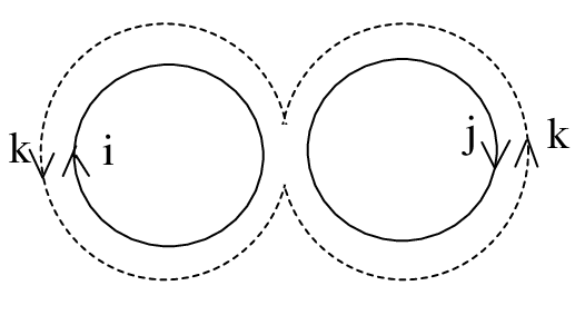
3.2 Bosonic quiver gauge theory in four dimensions

Let us start by considering the bosonic quiver gauge theory with $SU(N)\times SU(M)$ gauge group. As in the previous subsection, we take the limit $N,M\to\infty$ with $M=km$ , $N=kn$ , $k\to\infty$ and $m,n$ kept fixed. (As we will see, in terms of QCD with fundamental matter, this means $N_{c},N_{f}\to\infty$ with $N_{f}/N_{c}$ fixed.) Let us consider the action

$\displaystyle S$	$\displaystyle=$	$\displaystyle S_{gauge}+S_{matter}=\int dt\int_{S^{3}}d^{3}x\sqrt{g(x)}\left({\cal L}_{gauge}+{\cal L}_{matter}\right),$	(57)
$\displaystyle{\cal L}_{gauge}$	$\displaystyle=$	$\displaystyle-\frac{1}{4g_{A}^{2}}TrF_{\mu\nu}^{2}-\frac{1}{4g_{B}^{2}}TrG_{\mu\nu}^{2},$	(58)
$\displaystyle{\cal L}_{matter}$	$\displaystyle=$	$\displaystyle k\left(-Tr(D_{\mu}\phi_{I})(D^{\mu}\phi_{I})^{\dagger}+m_{IJ}Tr\phi_{I}\phi^{\dagger}_{J}\right),$	(59)

where $F_{\mu\nu}$ and $G_{\mu\nu}$ are field strength of $SU(N)$ and $SU(M)$ gauge fields $A_{\mu}$ and $B_{\mu}$ ,

\displaystyle F_{\mu\nu}=\partial_{\mu}A_{\nu}-\partial_{\nu}A_{\mu}-i[A_{\mu},A_{\nu}],\qquad G_{\mu\nu}=\partial_{\mu}B_{\nu}-\partial_{\nu}B_{\mu}-i[B_{\mu},B_{\nu}],

(60)

and $\phi_{I}(I=1,\cdots,K)$ are $N\times M$ complex matrices on which the covariant derivative acts as

\displaystyle D_{\mu}\phi_{I}=\partial_{\mu}\phi_{I}-iA_{\mu}\phi_{I}+i\phi_{I}B_{\mu}.

(61)

We take the mass matrix $m_{IJ}$ to be hermitian.

In the Maurer-Cartan basis, the matter part of the Lagrangian reads

\displaystyle{\cal L}_{matter}

\displaystyle=

\displaystyle kTr\Biggl\{(D_{t}\phi_{I})(D_{t}\phi_{I})^{\dagger}-(i\mu{\cal L}_{i}\phi_{I}-iA_{i}\phi_{I}+i\phi_{I}B_{i})(i\mu{\cal L}_{i}\phi_{I}-iA_{i}\phi_{I}+i\phi_{I}B_{i})^{\dagger}+m_{IJ}Tr\phi_{I}\phi^{\dagger}_{J}\Biggl\}.

The gauge part is the same as (24) for each gauge group.

By reducing the spatial dimensions to a point, we obtain

$\displaystyle S_{1d}$	$\displaystyle=$	$\displaystyle S_{1d}^{X}+S_{1d}^{Y}+S_{1d}^{matter},$	(63)
$\displaystyle S_{1d}^{X}$	$\displaystyle=$	$\displaystyle\frac{C}{g_{A}^{2}}\int dtTr\left(\frac{1}{2}(D_{t}X_{i})^{2}+\frac{1}{4}[X_{i},X_{j}]^{2}+i\mu\epsilon_{ijk}X^{i}X^{j}X^{k}-\frac{\mu^{2}}{2}X_{i}^{2}\right),$	(64)
$\displaystyle S_{1d}^{Y}$	$\displaystyle=$	$\displaystyle\frac{C}{g_{B}^{2}}\int dtTr\left(\frac{1}{2}(D_{t}Y_{i})^{2}+\frac{1}{4}[Y_{i},Y_{j}]^{2}+i\mu\epsilon_{ijk}Y^{i}Y^{j}Y^{k}-\frac{\mu^{2}}{2}Y_{i}^{2}\right),$	(65)
$\displaystyle S_{1d}^{matter}$	$\displaystyle=$	$\displaystyle Ck\int dtTr\Biggl\{(D_{t}\phi_{I})(D_{t}\phi_{I})^{\dagger}-(X_{i}\phi_{I}-\phi_{I}Y_{i})(X_{i}\phi_{I}-\phi_{I}Y_{i})^{\dagger}+m_{IJ}Tr\phi_{I}\phi^{\dagger}_{J}\Biggl\},$	(66)

where $X_{i}$ and $Y_{i}$ are $N\times N$ and $M\times M$ scalar matrices which are obtained from $A_{i}$ and $B_{i}$ . We take the background to be multiple of the background (2.2.2) as in (48),

\displaystyle X_{i}^{b.g.}=-\mu L_{i}\otimes\textbf{1}_{n},\qquad Y_{i}^{b.g.}=-\mu L_{i}\otimes\textbf{1}_{m},

(67)

where the size of $L_{i}$ is $k\times k$ . Then, it is straightforward to see that the Eguchi-Kawai equivalence works around this vacuum. By taking $g_{B}^{2}k$ to be zero, $SU(M)$ reduces to (a part of) a global “flavor” symmetry. The number of flavors turns out to be $N_{f}=MK$ , and the ratio $N_{f}/N_{c}$ can be arbitrary finite value.

3.3 Supersymmetric quiver gauge theory in four dimensions

We consider a quiver theory without superpotential. (incorporation of the superpotential is straightforward.) In this section we use the notation of Wess-Bagger’s textbook [40].

The action is given by

$\displaystyle S$	$\displaystyle=$	$\displaystyle S_{gauge}+S_{matter}=\int dt\int_{S^{3}}d^{3}x\sqrt{g(x)}\left({\cal L}_{gauge}+{\cal L}_{matter}\right),$	(68)
$\displaystyle{\cal L}_{gauge}$	$\displaystyle=$	$\displaystyle Tr\left\{-\frac{1}{g_{A}^{2}}\left(\frac{1}{4}F_{\mu\nu}^{2}+i\bar{\lambda}_{A}\bar{\sigma}^{\mu}D_{\mu}\lambda_{A}\right)-\frac{1}{g_{B}^{2}}\left(\frac{1}{4}G_{\mu\nu}^{2}+i\bar{\lambda}_{B}\bar{\sigma}^{\mu}D_{\mu}\lambda_{B}\right)\right\},$	(69)
$\displaystyle{\cal L}_{matter}$	$\displaystyle=$	$\displaystyle kTr\Biggl\{-(D_{\mu}\phi_{I})(D^{\mu}\phi_{I})^{\dagger}-i\bar{\psi_{I}}\bar{\sigma}^{\mu}D_{\mu}\psi_{I}-i\sqrt{2}\phi^{\dagger}_{I}(\lambda_{A}\psi_{I}-\psi_{I}\lambda_{B})$
		$\displaystyle\qquad+i\sqrt{2}(\bar{\psi}_{I}\bar{\lambda}_{A}-\bar{\lambda}_{B}\bar{\psi}_{I})\phi_{I}-\frac{k}{2}\left(g_{A}^{2}\phi_{I}\phi_{I}^{\dagger}\phi_{J}\phi_{J}^{\dagger}+g_{B}^{2}\phi^{\dagger}_{I}\phi_{I}\phi^{\dagger}_{J}\phi_{J}\right)-\frac{\mu^{2}}{8}(\phi_{I}\phi^{\dagger}_{I})\Biggl\},$

where $\psi_{I}$ and $\phi_{I}$ belong to $(N,\bar{M})$ representation as in the previous subsection. (Strictly speaking other multiplets are needed in order to cancel the gauge anomaly, but we omit them for notational simplicity. The modification is straightforward.) We notice that the last term is analogous to a mass term of adjoint scalars in 4d ${\cal N}=4$ on $S^{3}$ .

The supersymmetry transformation is

$\displaystyle\delta^{(4d)}A_{\mu}$	$\displaystyle=$	$\displaystyle-i\bar{\lambda}_{A}\bar{\sigma}_{\mu}\epsilon+i\bar{\epsilon}\bar{\sigma}_{\mu}\lambda_{A},$
$\displaystyle\delta^{(4d)}\lambda_{A}$	$\displaystyle=$	$\displaystyle F_{\mu\nu}\sigma^{\mu\nu}\epsilon+ikg_{A}^{2}\phi_{I}\phi_{I}^{\dagger}\epsilon,$
$\displaystyle\delta^{(4d)}B_{\mu}$	$\displaystyle=$	$\displaystyle-i\bar{\lambda}_{B}\bar{\sigma}_{\mu}\epsilon+i\bar{\epsilon}\bar{\sigma}_{\mu}\lambda_{B},$
$\displaystyle\delta^{(4d)}\lambda_{B}$	$\displaystyle=$	$\displaystyle G_{\mu\nu}\sigma^{\mu\nu}\epsilon+ikg_{B}^{2}\phi^{\dagger}_{I}\phi_{I}\epsilon,$
$\displaystyle\delta^{(4d)}\phi_{I}$	$\displaystyle=$	$\displaystyle\sqrt{2}\epsilon\psi_{I},$
$\displaystyle\delta^{(4d)}\psi_{I}$	$\displaystyle=$	$\displaystyle i\sqrt{2}\sigma^{\mu}\bar{\epsilon}D_{\mu}\phi_{I}+\frac{\mu}{4\sqrt{2}}\bar{\epsilon}\phi_{I}.$	(71)

Here the supersymmetry transformation parameter $\epsilon$ satisfies

\displaystyle D_{\mu}\epsilon=-\frac{i\mu}{4}\sigma_{\mu}\epsilon.

(72)

The dimensionally reduced model is obtained by rewriting the action in the Maurer-Cartan basis and then by reducing the spatial dimensions. It is important that the parameters of the supersymmetry transformation depends only on $t$ in this basis

\displaystyle\epsilon(t)=e^{-i\mu t/4}\epsilon_{0}.

(73)

Consequently the dimensional reduction of spatial dimensions does not affect supersymmetry.

By dimensionally reducing the spatial directions we obtain the matrix quantum mechanics

$\displaystyle L_{gauge}^{m.m.}$	$\displaystyle=$	$\displaystyle\frac{C}{g_{A}^{2}}Tr\Biggl(\frac{1}{2}\left(D_{t}X_{i}\right)^{2}+\frac{1}{4}[X_{i},X_{j}]^{2}-\frac{\mu^{2}}{2}X_{i}^{2}+i\mu\epsilon^{ijk}X_{i}X_{j}X_{k}\Biggl)$	(74)
		$\displaystyle+\frac{C}{g_{A}^{2}}Tr\left(-i\bar{\lambda}_{X}D_{t}\lambda_{X}-\bar{\lambda}_{X}\bar{\sigma}^{i}[X_{i},\lambda_{X}]-\frac{3}{4}\mu\bar{\lambda}_{X}\lambda_{X}\right)$
		$\displaystyle+(X\to Y),$

$\displaystyle L_{matter}^{m.m.}$	$\displaystyle=$	$\displaystyle CkTr\Biggl\{(D_{t}\phi_{I})(D_{t}\phi_{I})^{\dagger}-(X_{i}\phi_{I}-\phi_{I}Y_{i})(X_{i}\phi_{I}-\phi_{I}Y_{i})^{\dagger}$
		$\displaystyle\qquad-i\bar{\psi}_{I}D_{t}\psi_{I}-\bar{\psi}_{I}\bar{\sigma}^{i}(X_{i}\psi_{I}-\psi_{I}Y_{i})-\frac{3}{4}\mu\bar{\psi}_{I}\psi_{I}$
		$\displaystyle\qquad-i\sqrt{2}\phi^{\dagger}_{I}(\lambda_{X}\psi_{I}-\psi_{I}\lambda_{Y})+i\sqrt{2}(\bar{\psi}_{I}\bar{\lambda}_{X}-\bar{\lambda}_{Y}\bar{\psi}_{I})\phi_{I}$
		$\displaystyle\qquad-\frac{k}{2}\left(g_{A}^{2}\phi_{I}\phi_{I}^{\dagger}\phi_{J}\phi_{J}^{\dagger}+g_{B}^{2}\phi^{\dagger}_{I}\phi_{I}\phi^{\dagger}_{J}\phi_{J}\right)-\frac{\mu^{2}}{8}(\phi_{I}\phi^{\dagger}_{I})\Biggl\}.$

The supersymmetry transformation reduces to

$\displaystyle\delta^{(1d)}X_{i}$	$\displaystyle=$	$\displaystyle-i\bar{\lambda}_{X}\bar{\sigma}_{i}\epsilon+i\bar{\epsilon}\bar{\sigma}_{i}\lambda_{X},$
$\displaystyle\delta^{(1d)}A_{t}$	$\displaystyle=$	$\displaystyle-i\bar{\lambda}_{X}\epsilon+i\bar{\epsilon}\lambda_{X},$
$\displaystyle\delta^{(1d)}\lambda_{X}$	$\displaystyle=$	$\displaystyle\left[-2(D_{t}X_{i})+\epsilon^{ijk}[X_{j},X_{k}]+2i\mu X_{i}\right]\sigma^{i}\epsilon+ikg_{A}^{2}\phi_{I}\phi_{I}^{\dagger}\epsilon,$
$\displaystyle\delta^{(1d)}Y_{i}$	$\displaystyle=$	$\displaystyle-i\bar{\lambda}_{Y}\bar{\sigma}_{i}\epsilon+i\bar{\epsilon}\bar{\sigma}_{i}\lambda_{Y},$
$\displaystyle\delta^{(1d)}B_{t}$	$\displaystyle=$	$\displaystyle-i\bar{\lambda}_{Y}\epsilon+i\bar{\epsilon}\lambda_{Y},$
$\displaystyle\delta^{(1d)}\lambda_{B}$	$\displaystyle=$	$\displaystyle\left[-2(D_{t}Y_{i})+\epsilon^{ijk}[Y_{j},Y_{k}]+2i\mu Y_{i}\right]\sigma^{i}\epsilon+ikg_{B}^{2}\phi^{\dagger}_{I}\phi_{I}\epsilon,$
$\displaystyle\delta^{(1d)}\phi_{I}$	$\displaystyle=$	$\displaystyle\sqrt{2}\epsilon\psi_{I},$
$\displaystyle\delta^{(1d)}\psi_{I}$	$\displaystyle=$	$\displaystyle\sqrt{2}\sigma^{i}\bar{\epsilon}(X_{i}\phi_{I}-\phi_{I}Y_{i})+\frac{\mu}{4\sqrt{2}}\bar{\epsilon}\phi_{I},$	(76)

where $\epsilon$ is time-dependent

\displaystyle\epsilon(t)=e^{-i\mu t/4}\epsilon_{0}.

(77)

It turns out that the background (67) preserve this supersymmetry. By expanding the matrix model around this background we recover the original 4d theory. Notice that we have to renormalize the bare ’t Hooft couplings $g_{A}^{2}N$ and $g_{B}^{2}M$ appropriately in the continuum limit.

Generalizations to more complicated quiver theories are straightforward. We emphasize that the equivalence works only when the field theory does not has gauge anomalies, because we assumed implicitly in the proof.

The emergence of the chiral anomaly is a long standing problem in Eguchi-Kawai models. This problem exists in the present case too – the chiral symmetry seems kept in the reduced model. The chiral symmetry should be broken by some effect. Here, we do not pursue this direction, but just assume the presence of such an effect. One possible way to find it is to consider the chiral anomaly in the noncommutative space (concentric fuzzy spheres).

4 The Eguchi-Kawai model for Chern-Simons gauge theories

In this section, we consider the Eguchi-Kawai model of three dimensional Chern-Simons gauge theories. In a similar fashion to the YM cases, we can obtain matrix models which have a fuzzy sphere as a classical solution. Quivers can be introduced into this construction as in the previous section. We consider the ABJM model [14] as an example.

4.1 Bosonic case

Let us start with the bosonic Chern-Simons with $U(N)$ gauge group. The action is

\displaystyle S_{CS}

\displaystyle=

\displaystyle i\cdot\frac{k}{4\pi}\int d^{3}x\sqrt{g(x)}\epsilon^{\mu\nu\rho}Tr\left(-A_{\mu}\partial_{\nu}A_{\rho}-\frac{2i}{3}A_{\mu}A_{\nu}A_{\rho}\right),

(78)

where $k$ is an integer. On the three-sphere of radius $2/\mu$ , by using the Maurer-Cartan basis, this action can be written as [25]

\displaystyle S_{CS}

\displaystyle=

\displaystyle i\cdot\frac{k}{4\pi}\left(\frac{2}{\mu}\right)^{3}\int d^{3}\Omega Tr\left[\epsilon^{ijk}\left(\frac{i\mu}{2}\left(-({\cal L}_{i}A_{j})A_{k}+({\cal L}_{j}A_{i})A_{k}\right)-\frac{2i}{3}A_{i}A_{j}A_{k}\right)+\mu A_{i}^{2}\right].

Dimensionally reducing it, we obtain

\displaystyle S_{mm}=iC\cdot\frac{k}{4\pi}Tr\left(-\frac{2i}{3}\epsilon^{\mu\nu\rho}X_{\mu}X_{\nu}X_{\rho}+\mu X_{i}^{2}\right).

(80)

This theory has a classical solution

\displaystyle X_{i}=-\mu L_{i},\qquad[L_{i},L_{j}]=i\epsilon_{ijk}L_{k}.

(81)

It is easy to check that the 3d action () is obtained from (80) by taking the background (2.2.2) and using the mapping rule given in § 2.2.

4.2 ABJM theory

The previous construction can be easily promoted to supersymmetric Chern-Simons theory. As a concrete example, let us formulate the ABJM model, which gives a description of the multiple M2-branes theory [14] (see also [41]). In the following we take the gauge group to be $U(N)\times U(M)$ . When this model is put on the three sphere, an additional mass term must be added in order to keep supersymmetry. The model is given by

	$\displaystyle{\cal L}$	$\displaystyle=$	$\displaystyle\frac{ik}{4\pi}\epsilon^{\mu\nu\rho}Tr\left(-A_{\mu}\partial_{\nu}A_{\rho}-\frac{2i}{3}A_{\mu}A_{\nu}A_{\rho}+B_{\mu}\partial_{\nu}B_{\rho}+\frac{2i}{3}B_{\mu}B_{\nu}B_{\rho}\right)$		(82)
			$\displaystyle+\frac{k}{2\pi}Tr\left(D_{\mu}\bar{\phi}^{\alpha}D^{\mu}\phi_{\alpha}+i\bar{\psi}_{\alpha}\sigma^{\mu}D_{\mu}\psi^{\alpha}\right)+k{\cal V}(\phi,\psi),$		(82)

where

$\displaystyle{\cal V}(\phi,\psi)$	$\displaystyle=$	$\displaystyle-\frac{i}{2\pi}\epsilon^{\alpha\beta\gamma\delta}Tr\left(\phi_{\alpha}\bar{\psi}_{\beta}\phi_{\gamma}\bar{\psi}_{\delta}\right)+\frac{i}{2\pi}\epsilon_{\alpha\beta\gamma\delta}Tr\left(\bar{\phi}^{\alpha}\psi^{\beta}\bar{\phi}^{\gamma}\psi^{\delta}\right)$	(83)
		$\displaystyle-\frac{i}{2\pi}Tr\left(\bar{\phi}^{\alpha}\phi_{\alpha}\bar{\psi}_{\beta}\psi^{\beta}-\phi_{\alpha}\bar{\phi}^{\alpha}\psi^{\beta}\bar{\psi}_{\beta}+2\bar{\phi}^{\alpha}\psi^{\beta}\bar{\psi}_{\alpha}\phi_{\beta}-2\phi_{\alpha}\bar{\psi}_{\beta}\psi^{\alpha}\bar{\phi}^{\beta}\right)$
		$\displaystyle-\frac{1}{6\pi}Tr\left((\phi_{\alpha}\bar{\phi}^{\alpha})^{3}+(\bar{\phi}^{\alpha}\phi_{\alpha})^{3}\right)-\frac{2}{3\pi}Tr\left(\phi_{\alpha}\bar{\phi}^{\gamma}\phi_{\beta}\bar{\phi}^{\alpha}\phi_{\gamma}\bar{\phi}^{\beta}\right)$
		$\displaystyle+\frac{1}{\pi}Tr\left(\phi_{\alpha}\bar{\phi}^{\alpha}\phi_{\beta}\bar{\phi}^{\gamma}\phi_{\gamma}\bar{\phi}^{\beta}\right)+\frac{3\mu^{2}}{32\pi}\bar{\phi}^{\alpha}\phi_{\alpha}.$

Here $A_{\mu}$ and $B_{\mu}$ are gauge fields of $U(N)$ and $U(M)$ groups, respectively. Bifundamental matter fields $\phi_{\alpha},\psi^{\alpha}$ ( $\alpha=1,\cdots,4$ ) are in the $(N,\bar{M})$ representations and the covariant derivative $D_{\mu}$ acts as

\displaystyle D_{\mu}\phi_{\alpha}=\nabla_{\mu}\phi_{\alpha}-iA_{\mu}\phi_{\alpha}+i\phi_{\alpha}B_{\mu},

(84)

and similarly for $\psi^{\alpha}$ . We have rescaled these matter fields in such a way that the Chern-Simons level $k$ appears only in the overall factor.

The supersymmetry transformation is

$\displaystyle\delta^{(3d)}\phi_{\alpha}$	$\displaystyle=$	$\displaystyle-i\eta_{\alpha\beta}\psi^{\beta},$
$\displaystyle\delta^{(3d)}A_{\mu}$	$\displaystyle=$	$\displaystyle-\left(\eta^{\alpha\beta}\sigma_{\mu}\phi_{\alpha}\bar{\psi}_{\beta}+\eta_{\alpha\beta}\sigma_{\mu}\psi^{\beta}\bar{\phi}^{\alpha}\right),$
$\displaystyle\delta^{(3d)}B_{\mu}$	$\displaystyle=$	$\displaystyle-\left(\eta^{\alpha\beta}\sigma_{\mu}\bar{\psi}_{\beta}\phi_{\alpha}+\eta_{\alpha\beta}\sigma_{\mu}\bar{\phi}^{\alpha}\psi^{\beta}\right),$
$\displaystyle\delta^{(3d)}\psi^{\alpha}$	$\displaystyle=$	$\displaystyle\left[\sigma^{\mu}D_{\mu}\phi_{\gamma}-\frac{2}{3}\phi_{[\beta}\bar{\phi}^{\beta}\phi_{\gamma]}\right]\eta^{\gamma\alpha}+\frac{4}{3}\phi_{\beta}\bar{\phi}^{\alpha}\phi_{\gamma}\eta^{\gamma\beta}+\frac{2}{3}\epsilon^{\alpha\beta\gamma\delta}\phi_{\beta}\bar{\phi}^{\rho}\phi_{\gamma}\eta_{\delta\rho}-\frac{i\mu}{4}\eta^{\gamma\alpha}\phi_{\gamma},$

where the parameter satisfies $\eta^{\alpha\beta}=-\eta^{\beta\alpha}$ , $(\eta_{\alpha\beta})^{\ast}=\frac{1}{2}\eta^{\alpha\beta\gamma\delta}\eta_{\gamma\delta}=\eta^{\alpha\beta}$ and $\nabla_{\mu}\eta^{\alpha\beta}=-\frac{i\mu}{4}\sigma^{\mu}\eta^{\alpha\beta}$ .

Rewriting the action using the Maurer-Cartan basis and taking the zero-dimensional reduction, we obtain the matrix model

$\displaystyle S_{mm}$	$\displaystyle=$	$\displaystyle Ck\biggl[\frac{i}{4\pi}Tr\left(-\frac{2i}{3}\epsilon^{ijk}X_{i}X_{j}X_{k}+\mu X_{i}^{2}+\frac{2i}{3}\epsilon^{ijk}Y_{i}Y_{j}Y_{k}-\mu Y_{i}^{2}\right)$	(86)
		$\displaystyle-\frac{1}{2\pi}Tr(Y_{i}\bar{\phi}^{\alpha}-\bar{\phi}^{\alpha}X_{i})(X^{i}\phi_{\alpha}-\phi_{\alpha}Y^{i})$
		$\displaystyle+\frac{1}{2\pi}Tr\left(\bar{\psi}_{\alpha}\sigma^{i}\left(X_{i}\psi^{\alpha}-\psi^{\alpha}Y_{i}\right)+\frac{3\mu}{4}\bar{\psi}_{\alpha}\psi^{\alpha}\right)+{\cal V}(\phi,\psi)\biggl].$

Expanding this action around the background (2.2.2), we can reproduce the original action. As before, the transformation parameter in the 3d theory is a constant in the Maurer-Cartan basis and the reduced model is supersymmetric. The supersymmetry transformation is

$\displaystyle\delta^{(0d)}\phi_{\alpha}$	$\displaystyle=$	$\displaystyle-i\eta_{\alpha\beta}\psi^{\beta},$
$\displaystyle\delta^{(0d)}X_{i}$	$\displaystyle=$	$\displaystyle-\left(\eta^{\alpha\beta}\sigma_{i}\phi_{\alpha}\bar{\psi}_{\beta}+\eta_{\alpha\beta}\sigma_{i}\psi^{\beta}\bar{\phi}^{\alpha}\right),$
$\displaystyle\delta^{(0d)}Y_{i}$	$\displaystyle=$	$\displaystyle-\left(\eta^{\alpha\beta}\sigma_{i}\bar{\psi}_{\beta}\phi_{\alpha}+\eta_{\alpha\beta}\sigma_{i}\bar{\phi}^{\alpha}\psi^{\beta}\right),$
$\displaystyle\delta^{(0d)}\psi^{\alpha}$	$\displaystyle=$	$\displaystyle\left[\sigma^{i}(-iX_{i}\phi_{\gamma}+i\phi_{\gamma}Y_{i})-\frac{2}{3}\phi_{[\beta}\bar{\phi}^{\beta}\phi_{\gamma]}\right]\eta^{\gamma\alpha}+\frac{4}{3}\phi_{\beta}\bar{\phi}^{\alpha}\phi_{\gamma}\eta^{\gamma\beta}+\frac{2}{3}\epsilon^{\alpha\beta\gamma\delta}\phi_{\beta}\bar{\phi}^{\rho}\phi_{\gamma}\eta_{\delta\rho}-\frac{i\mu}{4}\eta^{\gamma\alpha}\phi_{\gamma}.$

Notice that this background preserves all supersymmetries.

In the actions the Chern-Simons level $k$ appears as an overall factor. The original ABJM is reproduced from the reduced model in the planar limit with both $k/N$ and $k/M$ kept fixed.

5 Conclusion and Discussions

In this paper we have applied a recently proposed large- $N$ reduction technique [16] to supersymmetric quiver and Chern-Simons theories. As concrete examples we have constructed the $SU(N)\times SU(M)$ supersymmetric quiver gauge theory with bifundamental matter fields and the ABJM model of multiple M2 branes. Furthermore, by taking one of the gauge couplings to be small in the supersymmetric quiver gauge theory we obtain $SU(N)$ supersymmetric QCD with flavor. In this construction both $N_{c}$ and $N_{f}$ are infinite but the ratio $N_{f}/N_{c}$ can take any value. Therefore this construction provides us with a valuable tool to study the dynamics of supersymmetric QCD, e.g. supersymmetry breaking, Seiberg duality conjecture [42], etc.

The reduced model of the ABJM theory will be useful to study the AdS/CFT correspondence numerically. Of particular interest is the strong ’t Hooft coupling region that is expected to describe type IIA string on $AdS^{4}\times{\mathbb{C}P}^{3}$ . This region can be studied by using the Eguchi-Kawai equivalence. It turns out that the parameter region where $k$ is smaller than $O(N)$ is also important to obtain insights into M-theory. Thermodynamical properties are also interesting. For these reasons it is still valuable to study a lattice formulation which is valid at finite- $N$ and can be put at finite temperature. For references in this direction, see e.g. [43].

We expect that these models have the sign problem, unlikely to the reduced model for 4d ${\cal N}=1$ pure SYM [22]. This problem possibly make it difficult to study these models numerically. At finite temperature, however, the sign problem might be mild, similarly to the case of the maximally supersymmetric matrix quantum mechanics [10]. It is important to study by direct simulation how severe the sign problem is.

Although inherently restricted to the planar limit, the Eguchi-Kawai equivalence can be a powerful tool to explore the dynamics of supersymmetric gauge theories. Numerical studies on these models will be reported in future communications.

Acknowledgments

The authors are grateful to G. Ishiki, J. Nishimura and H. Suzuki for stimulating discussions and comments. The authors thank the Yukawa Institute for Theoretical Physics at Kyoto University and participants of the YITP workshop YITP-W-09-04 on “Development of Quantum Field Theory and String Theory” who gave us useful comments.

References

[1] J. Giedt, R. Brower, S. Catterall, G. T. Fleming and P. Vranas, “Lattice super-Yang-Mills using domain wall fermions in the chiral limit,” Phys. Rev. D 79, 025015 (2009) [arXiv:0810.5746 [hep-lat]]. M. G. Endres, “Dynamical simulation of N=1 supersymmetric Yang-Mills theory with domain wall fermions,” arXiv:0902.4267 [hep-lat].
[2] J. Giedt, “Advances and applications of lattice supersymmetry,” PoS LAT2006, 008 (2006) [arXiv:hep-lat/0701006]. S. Catterall, D. B. Kaplan and M. Unsal, “Exact lattice supersymmetry,” arXiv:0903.4881 [hep-lat].
[3] T. Banks, W. Fischler, S. H. Shenker and L. Susskind, “M theory as a matrix model: A conjecture,” Phys. Rev. D 55 (1997) 5112; hep-th/9610043.
[4] N. Ishibashi, H. Kawai, Y. Kitazawa and A. Tsuchiya, “A large-N reduced model as superstring,” Nucl. Phys. B 498 (1997) 467; hep-th/9612115.
[5] R. Dijkgraaf, E. P. Verlinde and H. L. Verlinde, “Matrix string theory,” Nucl. Phys. B 500, 43 (1997); hep-th/9703030.
[6] J. M. Maldacena, “The large N limit of superconformal field theories and supergravity,” Adv. Theor. Math. Phys. 2 (1998) 231 [Int. J. Theor. Phys. 38 (1999) 1113]; hep-th/9711200.
[7] N. Itzhaki, J. M. Maldacena, J. Sonnenschein and S. Yankielowicz, “Supergravity and the large N limit of theories with sixteen supercharges,” Phys. Rev. D 58, 046004 (1998) [arXiv:hep-th/9802042].
[8] M. Hanada, J. Nishimura and S. Takeuchi, “Non-lattice simulation for supersymmetric gauge theories in one dimension,” Phys. Rev. Lett. 99 (2007) 161602; arXiv:0706.1647 [hep-lat].
[9] S. Catterall and T. Wiseman, “Towards lattice simulation of the gauge theory duals to black holes and hot strings,” JHEP 0712 (2007) 104; arXiv:0706.3518 [hep-lat].
[10] K. N. Anagnostopoulos, M. Hanada, J. Nishimura and S. Takeuchi, “Monte Carlo studies of supersymmetric matrix quantum mechanics with sixteen supercharges at finite temperature,” Phys. Rev. Lett. 100 (2008) 021601; arXiv:0707.4454 [hep-th].
[11] S. Catterall and T. Wiseman, “Black hole thermodynamics from simulations of lattice Yang-Mills theory,” Phys. Rev. D 78, 041502 (2008); arXiv:0803.4273 [hep-th].
[12] M. Hanada, A. Miwa, J. Nishimura and S. Takeuchi, “Schwarzschild radius from Monte Carlo calculation of the Wilson loop in supersymmetric matrix quantum mechanics,” arXiv:0811.2081 [hep-th]. M. Hanada, Y. Hyakutake, J. Nishimura and S. Takeuchi, “Higher derivative corrections to black hole thermodynamics from supersymmetric matrix quantum mechanics,” arXiv:0811.3102 [hep-th].
[13] J. H. Schwarz, “Superconformal Chern-Simons theories,” JHEP 0411, 078 (2004) [arXiv:hep-th/0411077].
[14] O. Aharony, O. Bergman, D. L. Jafferis and J. Maldacena, “N=6 superconformal Chern-Simons-matter theories, M2-branes and their gravity duals,” JHEP 0810, 091 (2008) [arXiv:0806.1218 [hep-th]].
[15] T. Eguchi and H. Kawai, “Reduction Of Dynamical Degrees Of Freedom In The Large N Gauge Theory,” Phys. Rev. Lett. 48 (1982) 1063.
[16] T. Ishii, G. Ishiki, S. Shimasaki and A. Tsuchiya, “N=4 Super Yang-Mills from the Plane Wave Matrix Model,” Phys. Rev. D 78, 106001 (2008) [arXiv:0807.2352 [hep-th]].
[17] P. Kovtun, M. Unsal and L. G. Yaffe, “Volume independence in large N(c) QCD-like gauge theories,” JHEP 0706, 019 (2007) [arXiv:hep-th/0702021].
[18] B. Bringoltz, “Large-N volume reduction of lattice QCD with adjoint Wilson fermions at weak-coupling,” arXiv:0905.2406 [hep-lat].
[19] P. F. Bedaque, M. I. Buchoff, A. Cherman and R. P. Springer, “Can fermions save large N dimensional reduction?,” arXiv:0904.0277 [hep-th].
[20] D. E. Berenstein, J. M. Maldacena and H. S. Nastase, “Strings in flat space and pp waves from N = 4 super Yang Mills,” JHEP 0204, 013 (2002) [arXiv:hep-th/0202021].
[21] G. Ishiki, S. W. Kim, J. Nishimura and A. Tsuchiya, “Deconfinement phase transition in ${\cal N}=4$ super Yang-Mills theory on $R\times S^{3}$ from supersymmetric matrix quantum mechanics,” Phys. Rev. Lett. 102, 111601 (2009) [arXiv:0810.2884 [hep-th]]. Y. Kitazawa and K. Matsumoto, “N=4 Supersymmetric Yang-Mills on $S^{3}$ in Plane Wave Matrix Model at Finite Temperature,” Phys. Rev. D 79, 065003 (2009) [arXiv:0811.0529 [hep-th]]. G. Ishiki, S. W. Kim, J. Nishimura and A. Tsuchiya, “Testing a novel large-N reduction for N=4 super Yang-Mills theory on $RxS^{3}$ ,” arXiv:0907.1488 [hep-th].
[22] M. Hanada, L. Mannelli and Y. Matsuo, “Four-dimensional N=1 super Yang-Mills from matrix model,” arXiv:0905.2995 [hep-th].
[23] N. Kim and J. H. Park, “Massive super Yang-Mills quantum mechanics: Classification and the relation to supermembrane,” Nucl. Phys. B 759, 249 (2006) [arXiv:hep-th/0607005].
[24] A. Armoni, M. Shifman and G. Veneziano, “Exact results in non-supersymmetric large N orientifold field theories,” Nucl. Phys. B 667, 170 (2003) [arXiv:hep-th/0302163]. A. Armoni, M. Shifman and G. Veneziano, “SUSY relics in one-flavor QCD from a new 1/N expansion,” Phys. Rev. Lett. 91, 191601 (2003) [arXiv:hep-th/0307097].
[25] T. Ishii, G. Ishiki, K. Ohta, S. Shimasaki and A. Tsuchiya, “On relationships among Chern-Simons theory, BF theory and matrix model,” Prog. Theor. Phys. 119, 863 (2008) [arXiv:0711.4235 [hep-th]].
[26] W. Taylor, “D-brane field theory on compact spaces,” Phys. Lett. B 394, 283 (1997) [arXiv:hep-th/9611042].
[27] G. Ishiki, K. Ohta, S. Shimasaki and A. Tsuchiya, to appear.
[28] G. Bhanot, U. M. Heller and H. Neuberger, “The Quenched Eguchi-Kawai Model,” Phys. Lett. B 113, 47 (1982).
[29] G. Parisi, “A Simple Expression For Planar Field Theories,” Phys. Lett. B 112, 463 (1982). D. J. Gross and Y. Kitazawa, “A Quenched Momentum Prescription For Large N Theories,” Nucl. Phys. B 206, 440 (1982). S. R. Das and S. R. Wadia, “Translation Invariance And A Reduced Model For Summing Planar Diagrams In QCD,” Phys. Lett. B 117, 228 (1982) [Erratum-ibid. B 121, 456 (1983)].
[30] H. Kawai and M. Sato, “Perturbative Vacua from IIB Matrix Model,” Phys. Lett. B 659, 712 (2008) [arXiv:0708.1732 [hep-th]].
[31] G. Ishiki, S. Shimasaki, Y. Takayama and A. Tsuchiya, “Embedding of theories with $SU(2|4)$ symmetry into the plane wave matrix model,” JHEP 0611, 089 (2006) [arXiv:hep-th/0610038].
[32] M. Hanada, H. Kawai and Y. Kimura, “Describing curved spaces by matrices,” Prog. Theor. Phys. 114, 1295 (2006) [arXiv:hep-th/0508211].
[33] A. Gonzalez-Arroyo and M. Okawa, “The Twisted Eguchi-Kawai Model: A Reduced Model For Large N Lattice Gauge Theory,” Phys. Rev. D 27 (1983) 2397.
[34] B. Bringoltz and S. R. Sharpe, “Breakdown of large-N quenched reduction in SU(N) lattice gauge theories,” arXiv:0805.2146 [hep-lat].
[35] T. Azeyanagi, M. Hanada, T. Hirata and T. Ishikawa, “Phase structure of twisted Eguchi-Kawai model,” JHEP 0801 (2008) 025; arXiv:0711.1925 [hep-lat].
[36] M. Teper and H. Vairinhos, “Symmetry breaking in twisted Eguchi-Kawai models,” Phys. Lett. B 652 (2007) 359; arXiv:hep-th/0612097.
[37] W. Bietenholz, J. Nishimura, Y. Susaki and J. Volkholz, “A non-perturbative study of 4d U(1) non-commutative gauge theory: The fate of one-loop instability,” JHEP 0610 (2006) 042; hep-th/0608072.
[38] T. Azeyanagi, M. Hanada and T. Hirata, “On Matrix Model Formulations of Noncommutative Yang-Mills Theories,” Phys. Rev. D 78, 105017 (2008) [arXiv:0806.3252 [hep-th]].
[39] M. Unsal and L. G. Yaffe, “Center-stabilized Yang-Mills theory: confinement and large $N$ volume independence,” arXiv:0803.0344 [hep-th].
[40] J. Wess and J. Bagger, “Supersymmetry and supergravity,”
[41] K. Hosomichi, K. M. Lee, S. Lee, S. Lee and J. Park, “N=5,6 Superconformal Chern-Simons Theories and M2-branes on Orbifolds,” JHEP 0809, 002 (2008) [arXiv:0806.4977 [hep-th]]. D. Gaiotto, S. Giombi and X. Yin, “Spin Chains in N=6 Superconformal Chern-Simons-Matter Theory,” JHEP 0904, 066 (2009) [arXiv:0806.4589 [hep-th]].
[42] N. Seiberg, “Electric - magnetic duality in supersymmetric nonAbelian gauge theories,” Nucl. Phys. B 435, 129 (1995) [arXiv:hep-th/9411149].
[43] F. Berruto, M. C. Diamantini and P. Sodano, “On pure lattice Chern-Simons gauge theories,” Phys. Lett. B 487 (2000) 366 [arXiv:hep-th/0004203]. C. D. Fosco and A. Lopez, “Generalized parity transformations in the regularized Chern-Simons theory,” Phys. Rev. D 64 (2001) 025017 [arXiv:hep-th/0102088]. W. Bietenholz, J. Nishimura and P. Sodano, “Chern-Simons theory on the lattice,” Nucl. Phys. Proc. Suppl. 119 (2003) 935 [arXiv:hep-lat/0207010].