Random effects compound Poisson model to represent data with extra zeros

Journal: Computational Statistics and Data Analysis

Marie-Pierre Étienne Corresponding author: Départment MMIP - Team Morse. 16 rue Claude Bernard, 75231 Paris Cedex 5. FRANCE URL: www.agroparistech.fr/morse/etienne.html Address: AgroParisTech, UMR 518, F-75000 Paris, France Address: INRA, UMR 518, F-75000 Paris, France Éric Parent Address: AgroParisTech, UMR 518, F-75000 Paris, France Address: INRA, UMR 518, F-75000 Paris, France Hugues Benoit Address: Fisheries and Oceans Canada, Moncton, New Brunswick,Canada Jacques Bernier Email: marie.etienne@agroparistech.fr Address: AgroParisTech, UMR 518, F-75000 Paris, France

August 24, 2026

Abstract

This paper describes a compound Poisson-based random effects structure for modeling zero-inflated data. Data with large proportion of zeros are found in many fields of applied statistics, for example in ecology when trying to model and predict species counts (discrete data) or abundance distributions (continuous data). Standard methods for modeling such data include mixture and two-part conditional models. Conversely to these methods, the stochastic models proposed here behave coherently with regards to a change of scale, since they mimic the harvesting of a marked Poisson process in the modeling steps. Random effects are used to account for inhomogeneity. In this paper, model design and inference both rely on conditional thinking to understand the links between various layers of quantities : parameters, latent variables including random effects and zero-inflated observations. The potential of these parsimonious hierarchical models for zero-inflated data is exemplified using two marine macroinvertebrate abundance datasets from a large scale scientific bottom-trawl survey. The EM algorithm with a Monte Carlo step based on importance sampling is checked for this model structure on a simulated dataset : it proves to work well for parameter estimation but parameter values matter when re-assessing the actual coverage level of the confidence regions far from the asymptotic conditions.

Keywords:

EM algorithm , Importance Sampling , Compound Poisson Process, Random Effect Model , zero-inflated Data

2008 MSC

62F12, 62P12, 62L12, 92D40, 92d50

1 Introduction

Often data contain a greater number of zero observations than would be predicted using standard, unimodal statistical distributions. This currently happens in ecology (see [16]) when counting species (over-dispersion for discrete data) or recording biomasses (atoms at zero for continuous data). Such data are generally referred to as zero-inflated data and require specialized treatments for statistical analysis (12). Common statistical approaches to modeling zero-inflated data make recourse either to mixture models, such as the Dirac function for the occurrence of extra zeros in addition to a standard probability distribution (see for instance [21]), or to two-part conditional models (a presence/absence Bernoulli component and some other distribution for non zero observations given presence such as in [25]). These models are well-known (4) and offer the advantages of separate fits and separate interpretations of each of their components. Parameters are well understood and interpreted as the probability of presence, and the average abundance of biomass if present.

However, a major flaw of those models is their non-additive behavior with regards to variation in within-experiment sampling effort (26). Consider for instance the fishing effort measured by the ground surface swept by a bottom-trawl during a scientific survey of benthic marine fauna. If during experiment $i$ , observation $Y_{i}$ is made with some experimental effort corresponding to the harvesting of some area $D_{i}$ and is assumed to stem from a stochastic model with parameters $\theta(D_{i})$ , then the additivity properties of coherence are naturally required: if we consider two (possibly subsequent) independent experiments $i$ and $i^{\prime}$ on the different non overlapping areas $D_{i}$ and $D_{i^{\prime}}$ , we would expect that the random quantity $Y_{i}+Y_{i^{\prime}}$ stems from the same stochastic model with parameters $\theta(D_{i}\cup D_{i^{\prime}})$ . A compound Poisson distribution is a sum of independent identically distributed random variables in which the number of terms in the sum has a Poisson distribution. Compound Poisson distributions are candidate models purposely tailored to verify the previous desired infinite divisibility property since the class of infinitely divisible distributions coincides with the class of limit distributions of compound Poisson distributions ([9], theorem 3 of chapter 27).

Depending on the nature of the term in the random sum, the compound distribution can be discrete or continuous. The construction of such a compound distribution with an exponential random mark for continuous data and with a geometric one for counts is recalled in section 2. This approach is worthwhile for two reasons. The first is parsimony : there is only one parameter for the Poisson distribution plus an additional one for the probability distribution function - pdf - of each component of the random sum. Secondly, the compound construction may assist our understanding in cases where the data collection can be interpreted in terms of sampling a latent marked Poisson field. That is to say that the data appear in latent "clumps" that are "harvested" during the experiment, the Poisson parameter being the presence intensity of such clumps. A random variable is used to mimic the quantity (or the number of individuals in the discrete case) independently in each clump. At the upper level of the hierarchy, random effects are added to depict heterogeneous conditions between blocks of experiments.

In section 3, we develop a stochastic version of the EM algorithm (7) with a Monte-Carlo step (using importance sampling) for this non Gaussian random effect model with zero-inflated data. Maximum likelihood estimates and the corresponding variance-covariance matrix are derived. The computational task remains rather tractable thanks to simplifying gamma-exponential conjugate properties in the continuous case (and beta-geometric conjugacy in the discrete case).

In section 4, the hierarchical model (29) with compound Poisson distribution for zero-inflated data is exemplified using a real case study with two marine species, urchin and starfish abundance data from a scientific bottom-trawl survey of the southern Gulf of St. Lawrence, Canada. The EM algorithm performs well in obtaining the maximum likelihood estimates of parameters, but for one of the two species we notice some discrepancy between the actual coverage of the confidence intervals and their theoretical levels (as given by the asymptotic normal approximation). Consequently, we further focus on variance covariance matrix estimation in section 5 and investigate via simulation the behavior of coverage level of confidence intervals for various experimental designs, in search of a practical fulfillment of the asymptotic conditions. Finally, we briefly discuss some inferential and practical issues encountered when implementing such hierarchical models for zero-inflated data.

2 Model construction

We propose a hierarchical construction to represent data with extra zero collected over a non-homogeneous area. The model is divided into two main layers : in the first one, we model the sampling process within a homogeneous sub-area (strata) and in the second layer, we introduce heterogeneity between strata at the top of the hierarchy using random effects. The first subsections detail the hierarchical constructions for continuous data. In the last subsection 2.4, we sketch out an obvious modification to represent count data.

2.1 Compound Poisson process to introduce extra zeros

Imagine that data $Y$ are obtained by harvesting an area $D$ and that there are some clumps distributed according to an homogeneous Poisson process : clumps are uniformly distributed with a constant intensity, say $\mu$ .

By harvesting an area $D$ , we pick an integer-valued random variable $N$ of clumps. According to Poisson process property $N$ follows a Poisson distribution of parameter $\mu\,D$ . For each clump $i$ the independent random variables $X_{i}$ or marks (with the same probability distribution) represent for instance the possible biomass in each clump to be collected.
The final return will consist of the sum over $N$ clumps of the amount contained in each clump. With the convention that $Y=0$ if $N=0$ , the random sum :

Y=\sum_{i=0}^{N}X_{i},

(2.1)

is said to follow a compound Poisson distribution. Figure 1 exemplifies a realization of the total amount of a collect (i.e., sum of the marks) in a sampled region $D$ .

The Poisson-based additivity property avoids the drawback of classical models mentioned in the introduction. Generally, $D$ is the area of the sampled area included in $\mathbb{R}^{2}$ . We assume an homogeneous region $\mu(D)=\mu\,D$ , so that the expected number of collected clumps is proportional to the catching effort. The difficulty with the generalization to an inhomogeneous Poisson process lies in the inference step, not in the modeling step. Consequently we used another approach to deal with heterogeneity (see section 2.3). In the following, we mostly omit to index quantities with this catching effort for presentation clarity, explicitly mentioning it only when necessary.

Summary statistics about such compound distribution $Y$ are easily obtained (the characteristic function is given in appendix A) :

	$\displaystyle\mathbb{E}(Y)$	$\displaystyle=\mu\,D\ \mathbb{E}(X)$
	$\displaystyle\mathbb{V}ar(Y)$	$\displaystyle=\mu\,D\ \mathbb{E}(X^{2})$

Parameter $\mu$ rules the occurrence of zero values when assuming $\mathbb{P}(X=0)=0$ i.e. that the random mark is non atomic at $0$ :

\mathbb{P}(Y=0)=\exp{\left(-\mu\,D\right)}.

Refer to caption — Figure 1: Realization of a marked Poisson process on a region of $\mathbb{R}^{2}$ , the sample is conducted over a region $D$ . Here the total catch is $y=7.7$ , the effective number of collected clumps is $8$ .

2.2 Choice of the random component $X$ for continuous data

For real-valued data with extra zeros, we will concentrate in this paper on the exponential distribution of parameter $\rho$ for component $X$ such that $\mathbb{E}(X)=\rho^{-1}$ , leading to

\mathbb{E}(Y)=\frac{\mu\,D}{\rho}\quad\text{and}\quad\mathbb{V}ar(Y)=2\frac{\mu\,D}{\rho^{2}}.

To keep on with an ecological interpretation of the model, assuming that the mark $X$ follows an exponential distribution of parameter $\rho$ , means for the biologist that the probability of finding a large amount of biomass within a clump is exponentially decreasing and that the average quantity in each clump is $\rho^{-1}$ . When no clump is collected, there occurs a zero for the model $Y$ . We choose the exponential distribution because of parsimony and because of its interesting conjugate property detailed in section 3.1.2.

This compound Poisson distribution was termed law of leaks (LOL) by [6], where $X$ represents elementary unobserved leaks occurring at $N$ holes (uniformly located) along a gas pipeline. In summary :

\left(Y\sim LOL(\mu,\rho)\right)\Longleftrightarrow\left(\begin{array}[]{l}Y=\sum_{i=1}^{N}X_{j},\cr N\sim\mathcal{P}(\mu),\cr(X_{1},\ldots,X_{N})\overset{i.i.d}{\sim}\mathcal{E}(\rho)\end{array}\right)

(2.2)

For the discrete case, a similar definition holds with the corresponding geometric distribution for the marks (see section 2.4).

2.3 Random effects

Although the previous compound construction could have formally been extended to non-homogeneous Poisson processes, it is easier but still quite realistic to relax the assumption of homogeneity by considering homogeneous blocks (or strata), modeling possible inter-block dispersion using random effects. We consider $S$ blocks ; in a given block $s$ there are $I_{s}$ grouped observations. We denote by $\underline{Y_{s}}=(Y_{s\,1},\ldots,Y_{s\,I_{s}})$ the random vector in block $s$ and by $\underline{\mathbf{Y}}=(\underline{Y_{1}},\ldots,\underline{Y_{S}})$ the whole vector over the $S$ blocks. The coefficients $a$ and $b$ of the gamma pdf $\Gamma(a,b)$ for a random variable $\mu$ are such that $\mathbb{E}(\mu)=\frac{a}{b}$ and $\mathbb{V}ar(\mu)=\frac{a}{b^{2}}$ . The random effect model $RLOL(a,b,c,d)$ representing the occurrence of the sample $\underline{\mathbf{Y}}$ is defined by the following set of equations.

\underline{\mathbf{Y}}\sim RLOL(a,b,c,d)\Longleftrightarrow\left\{\begin{array}[c]{l}(\mu_{1},\ldots,\mu_{S})\overset{i.i.d}{\sim}\Gamma(a,b),\\ (\rho_{1},\ldots,\rho_{S})\overset{i.i.d}{\sim}\Gamma(c,d),\\ Y_{s,1},\ldots,Y_{s,I_{s}}\mid\mu_{s},\rho_{s}\overset{i}{\sim}LOL\left(\mu_{s}\,D_{s,k},\rho_{s}\right)\ \forall s\in\left\{1,\ldots,S\right\}.\end{array}\right.

(2.3)

The choice of a gamma distribution for the random effect is motivated by conjugate properties which are useful in the inference of the model. Section 4.1.3 will show that it may also be quite a realistic distribution for some datasets. The hierarchical construction is summed up by the directed acyclic graph (DAG as termed by [23]) in Figure 2.

2.4 Compound Poisson process for count data

A similar but discrete version to model count data, can be obtained by changing the nature of the random marks of the Poisson process. In this paper, we study a geometric distribution with parameter $p=\mathbb{P}(X=1)$ . The core of the model is thus given by the following compound Poisson process with geometric marks :

\left(Y\sim DLOL(\mu,p)\right)\Longleftrightarrow\left(\begin{array}[]{l}Y=\sum_{i=1}^{N}X_{j},\cr N\sim\mathcal{P}(\mu),\cr(X_{1},\ldots,X_{N})\overset{i.i.d}{\sim}\mathcal{G}(p)\end{array}\right)

To preserve conjugate properties, the gamma distribution for the random effect on the marks is replaced by a beta distribution so that the count data version of the model is given by :

\underline{\mathbf{Y}}\sim RDLOL(a,b,c,d)\Longleftrightarrow\left\{\begin{array}[c]{l}(\mu_{1},\ldots,\mu_{S})\overset{i.i.d}{\sim}\Gamma(a,b),\\ (p_{1},\ldots,p_{S})\overset{i.i.d}{\sim}\beta(c,d),\\ Y_{s,1},\ldots,Y_{s,I_{s}}\mid\mu_{s},p_{s}\overset{i}{\sim}DLOL(\mu_{s}D_{s,k},p_{s})\ \forall s\in\left\{1,\ldots,S\right\}.\end{array}\right.

(2.4)

where $DLOL$ means Discrete version of Law of leaks and $RDLOL$ discrete law of leaks with random effects.

In most of the paper, we will simply state the main results when technical aspects of the proofs are shared between discrete and continuous cases.

3 Estimation via the EM algorithm with importance sampling

Hierarchical models such as 2.3 or 2.4 cannot be straightforwardly estimated because of the latent variables. The random effects $(\mathbf{\mu},\mathbf{\rho})$ and the unknown numbers of clumps $\underline{\mathbf{N}}$ must be integrated out to obtain the likelihood. The likelihood has no closed form and estimators cannot be directly derived. In such a case, a classical strategy is to use Expectation Maximization algorithm ([7]) to derive max-likelihood estimates. In our case the E step is not analytically accessible. An alternative is to use a stochastic version of this EM algorithm such as Monte-Carlo EM ( MCEM see [18] or [19]) or stochastic approximation of EM (SAEM see [8]).

We detail in this section how to implement a MCEM algorithm using Importance sampling to obtain the maximum likelihood estimation and its empirical variance matrix. Similar results concerning count data process are summed up in the last subsection. From this point onwards we will use brackets to denote pdf’s as many conditioning terms will appear in the probabilistic expressions derived from the model fully specified by the set of equations (2.3). The brackets denote either a density or a discrete probability distribution, as in [10]. Following Bayesian conventions, we will also allow the parameters to appear as conditioning terms (i.e., instead of writing $\mathbb{P}(X)$ we will specify $[X|a,b,c,d]$ ) so as to help the reader understand which layer of the hierarchical model (2.3) the probability expression refers to (see Fig 2).

3.1 Implementation of the MCEM algorithm

In this paper, $\theta$ stands for the set of parameters $(a,b,c,d)$ in the $RLOL$ model. Given the random effects, the data within a block are independent :

L(\theta;\underline{\mathbf{Y}},\underline{\mathbf{N}},\mathbf{\mu},\mathbf{\rho})=\sum_{s=1}^{S}L_{s}

where $L_{s}$ denotes the complete log-likelihood in block $s$ , i.e. :

	$\displaystyle L_{s}=L_{s}(\theta;\underline{Y_{s}},\underline{N_{s}},\mu_{s},\rho_{s})$	$\displaystyle=\left(\sum_{i=1^{I_{s}}}\ln\left(\left[Y_{s,i}\|N_{s,i},\rho_{s}\right]\left[N_{s,i}\|\mu_{s}\right]\right)\right)+$		(3.1)
		$\displaystyle\hskip 28.45274pt\ln\left(\left[\mu_{s}\|a,b\right]\right)+\ln\left(\left[\rho_{s}\|c,d\right]\right)$

Following [28], the pivotal quantity in the EM algorithm (recalled in appendix D) is the conditional expectation of the complete log-likelihood :

Q(\theta,\theta^{\prime})=\mathbb{E}_{\theta^{\prime}}\left(L(\theta;\underline{\mathbf{Y}},\underline{\mathbf{N}},\mathbf{\mu},\mathbf{\rho})|\underline{\mathbf{Y}}\right)

3.1.1 Maximization step

To maximize $Q(\theta,\theta^{\prime})$ with respect to $\theta$ , we focus on the terms that involve $\theta$ :

	$\displaystyle Q(\theta,\theta^{\prime})$	$\displaystyle=C_{-\theta}(Y)+(a-1)\times\sum_{s=1}^{S}\mathbb{E}_{\theta^{\prime}}\left(\ln{\mu_{s}}\mid\underline{Y_{s}}\right)+Sa\ln{b}-b\sum_{s=1}^{S}\mathbb{E}_{\theta^{\prime}}\left(\mu_{s}\mid\underline{Y_{s}}\right)-S\ln(\Gamma(a))$
		$\displaystyle+(c-1)\times\sum_{s=1}^{S}\mathbb{E}_{\theta^{\prime}}\left(\ln{\rho_{s}}\mid\underline{Y_{s}}\right)+Sc\ln{d}-d\sum_{s=1}^{S}\mathbb{E}_{\theta^{\prime}}\left(\rho_{s}\mid\underline{Y_{s}}\right)-S\ln(\Gamma(c)),$		(3.2)

where $C_{-\theta}(Y)$ denotes a constant which does not depend on $\theta$ .

Differentiating with respect to $\theta$ , we obtain the set of equations to be satisfied at the maximum $\underset{\theta}{argmax\ }Q(\theta,\theta^{\prime})$ :

\frac{a}{b}=\frac{{\displaystyle\sum\limits_{s=1}^{S}}\mathbb{E}_{\theta^{\prime}}\left(\mu_{s}\mid\underline{Y_{s}}\right)}{S}

(3.3)

\ln{a}-\psi(a)=\ln{\left(\frac{{\displaystyle\sum\limits_{s=1}^{S}}\mathbb{E}_{\theta^{\prime}}\left(\mu_{s}\mid\underline{Y_{s}}\right)}{S}\right)}-\frac{{\displaystyle\sum\limits_{s=1}^{S}}\mathbb{E}_{\theta^{\prime}}\left(\ln{\mu_{s}}\mid\underline{Y_{s}}\right)}{S}

(3.4)

\frac{c}{d}=\frac{\displaystyle\sum\limits_{s=1}^{S}\mathbb{E}_{\theta^{\prime}}\left(\rho_{s}\mid\underline{Y_{s}}\right)}{S}

(3.5)

\ln{c}-\psi(c)=\ln{\left(\frac{{\displaystyle\sum\limits_{s=1}^{S}}\mathbb{E}_{\theta^{\prime}}\left(\rho_{s}\mid\underline{Y_{s}}\right)}{S}\right)}-\frac{{\displaystyle\sum\limits_{s=1}^{S}}\mathbb{E}_{\theta^{\prime}}\left(\ln{\rho_{s}}\mid\underline{Y_{s}}\right)}{S}

(3.6)

$\psi(x)$ denotes the digamma function defined as the first logarithmic derivative of $\Gamma(x)$ . No analytical expression can be derived for $\theta$ as the argument of the maximum of $Q(\theta,\theta^{\prime})$ , but a Newton-Raphson algorithm

is efficient and easy to implement with a good empirical starting point as indicated in annex B.

3.1.2 Expectation step by conditioning onto the number of clumps

The right-hand side of equations 3.3 to 3.6 involves $\mathbb{E}_{\theta^{\prime}}\left(\mu_{s}\mid\underline{Y_{s}}\right)$ , $\mathbb{E}_{\theta^{\prime}}\left(\ln(\mu_{s})\mid\underline{Y_{s}}\right)$ , $\mathbb{E}_{\theta^{\prime}}\left(\rho_{s}\mid\underline{Y_{s}}\right)$ and $\mathbb{E}_{\theta^{\prime}}\left(\ln(\rho_{s})\mid\underline{Y_{s}}\right).$ To compute these expected values, we will proceed by conditioning onto the hidden number of clumps $\underline{\mathbf{N}}$ . Proposition 3.1 shows that, given $\underline{\mathbf{N}},$ these four target quantities are simply marginal expectations of the sufficient quantity $N_{s+},$ the only necessary function of $\underline{\mathbf{N}}$ that needs to be evaluated within each block $s$ .

In a second step, integration over the number of clumps is performed by recourse to importance sampling within a block $s$ as detailed in proposition 3.3. Proofs of propositions are given in appendix E

Proposition 3.1.

Assuming $Y\sim RLOL(\theta^{\prime})$ with $\theta^{\prime}=(a^{\prime},b^{\prime},c^{\prime},d^{\prime})$ , $S$ strata and $I_{s}$ records in stratum $s$ as in 2.3 , then the complete conditional distributions of $\mu_{s}$ and $\rho_{s}$ in one particular stratum $s$ are given by

\mu_{s}|\underline{\mathbf{N}},\underline{\mathbf{Y}},\theta^{\prime}\sim\Gamma(a^{\prime}+N_{s+},b^{\prime}+D_{s+}),

(3.7)

and

\rho_{s}|\underline{\mathbf{N}},\underline{\mathbf{Y}},\theta^{\prime}\sim\Gamma(a^{\prime}+N_{s+},b^{\prime}+Y_{s+}),

(3.8)

where in stratum $s$ , $N_{s+}=\sum_{i=1}^{I_{s}}N_{si}$ denotes the total number of clumps caught, $Y_{s+}=\sum_{i=1}^{I_{s}}Y_{si}$ is the entire quantity harvested and $D_{s+}=\sum_{i=1}^{I_{s}}D_{si}$ is the whole catching effort.
The quantities involved in the E step are given by

$\displaystyle\mathbb{E}_{\theta^{\prime}}\left(\mu_{s}\mid\underline{y_{s}}\right)=$	$\displaystyle\frac{a^{\prime}+\mathbb{E}_{\theta^{\prime}}\left(N_{s+}\|\underline{y_{s}}\right)}{b^{\prime}+D_{s+}},$	(3.9)
$\displaystyle\mathbb{E}_{\theta^{\prime}}\left(\ln(\mu_{s})\mid\underline{y_{s}}\right)=$	$\displaystyle\mathbb{E}_{\theta^{\prime}}\left(\psi(a^{\prime}+N_{s+})\left\|\underline{y_{s}}\right.\right)-\ln(b^{\prime}+D_{s+}),$	(3.10)
$\displaystyle\mathbb{E}_{\theta^{\prime}}\left(\rho_{s}\mid\underline{y_{s}}\right)=$	$\displaystyle\frac{c^{\prime}+\mathbb{E}_{\theta^{\prime}}\left(N_{s+}\|\underline{y_{s}}\right)}{d^{\prime}+Y_{s+}},$	(3.11)
$\displaystyle\mathbb{E}_{\theta^{\prime}}\left(\ln(\rho_{s})\mid\underline{y_{s}}\right)=$	$\displaystyle\mathbb{E}_{\theta^{\prime}}\left(\psi(c^{\prime}+N_{s+})\left\|\underline{y_{s}}\right.\right)-\ln(d^{\prime}+Y_{s+}).$	(3.12)

This result merely comes from the conjugacy property between gamma and Poisson distributions for $\mu$ (gamma and exponential distribution concerning $\rho$ ). The moments of gamma and log gamma, beta and log beta distributions are recalled in appendix C.

In order to go one step further into the calculus, we have to perform the integration over $N_{+}$ . Proposition 3.2 gives the distribution of $N_{+}|Y_{+},\theta$ up to a constant. Subsequently, the integration over $N_{+}$ will make recourse to importance sampling as proposed in [15]. This Monte Carlo algorithm is detailed in proposition 3.3.

Proposition 3.2.

Assuming $Y\sim RLOL(a,b,c,d)$ with $S$ strata, and $I_{s}$ records in stratum $s$ , the conditional distribution of $\underline{N_{s}}|\theta,\underline{y_{s}}$ is given (up to a constant $K$ ) by

[\underline{N_{s}}|\theta^{\prime},\underline{y_{s}}]=K\,\left(\frac{\Gamma(a^{\prime}+N_{s+})\Gamma(c^{\prime}+N_{s+})}{b^{\prime}+D_{s+})^{N_{s+}}(d^{\prime}+Y_{s+})^{N_{s+}}}\right)\,\prod_{{\small i=1,\,y_{i}>0}}^{I_{s}}\left(\frac{y_{si}^{N_{si}}}{\Gamma(N_{si})\Gamma(N_{si}+1)}\right)\prod_{{\small i=1,\,y_{i}=0}}^{I_{s}}\delta(N_{si})

(3.13)

To draw a sample according to the rather intricate looking distribution 3.13, an importance sampling based algorithm is detailed in the following proposition for one replicate (often termed particle). In order to obtain a $G$ -sample, this procedure is repeated for each block $G$ times.

Proposition 3.3 (Generate one particle in one particular stratum $s$ according to distribution 3.13).

A particle $g$ is a vector $(N_{s+}^{(g)},N_{s1}^{(g)},\ldots,N_{sI_{s}}^{(g)})$ in a particular stratum $s$ . Omitting $s$ to make the reading easier, we may assume with no loss of generality that the first $I^{+}$ terms are non zero and the $I-I^{+}$ followings are the zero ones. The algorithm to generate one particle $g$ runs as follows:

1.

Generate $N_{i}^{(g)}=0$ wherever $y_{i=0}$ for $i=I-I^{+}+1,\ldots,I$ .

Generate the value of the random sum $N_{+}^{(g)}$ according to the importance distribution :

f_{IS}(N^{+})\varpropto\left(\frac{1}{b^{\prime}+D_{+}}\right)^{N^{+}}\left(\frac{Y^{+}}{d^{\prime}+Y^{+}}\right)^{N^{+}}\frac{\Gamma(a^{\prime}+N^{+})\Gamma(c^{\prime}+N^{+})}{\left(\prod_{i=1}^{I^{+}}\Gamma\left(\frac{y_{i}}{Y^{+}}N^{+}+1\right)\right)\Gamma\left(N_{+}-I_{+}+1\right)}

As the one dimensional importance distribution $f_{IS}$ is a quickly decreasing function of $N^{+}$ , its normalizing constant can be easily approximated and a bounded interval is used in practice as the support of $N^{+}$ .

3.

Generate each $N_{i}^{(g)}$ for $i=1,\ldots,I^{+}$ so that the vector $(N_{1}^{(g)}-1,\ldots,N_{I^{+}}^{(g)}-1)$ is distributed according to a multinomial distribution $\mathcal{M}(N_{+}^{(g)}-I_{+},(y_{1}/Y_{+},\ldots,y_{I^{+}}/Y_{+}))$ .
4.

Associate to the vector $(N_{+}^{(g)},N_{1}^{(g)},\ldots,N_{I}^{(g)})$ generated at the previous step, the importance weight :

$w^{(g)}=\prod_{i=1}^{I_{+}}\frac{\Gamma\left(N_{+}^{(g)}\frac{y_{i}}{Y_{+}}+1\right)}{\Gamma(N_{i}^{(g)}+1)}$

The proof of this proposition is straightforward from importance sampling theory (see for instance chapter 3 of [22]).

The weighted sample of $N_{+}$ may be used to approximate the expected conditional value defined in equations 3.9 to 3.12. For instance, quantity 3.10 is approximated by :

\mathbb{E}_{\theta^{\prime}}\left(\ln(\mu_{s})\mid\underline{y_{s}}\right)\approx\left(\frac{1}{\sum_{g=1}^{G}\omega^{(g)}}\sum_{g=1}^{G}\omega^{(g)}\times\psi(a^{\prime}+N_{s+}^{(g)})\right)-\ln(b^{\prime}+D_{s+}).

3.1.3 Empirical Variance Matrix

This section is devoted to the evaluation of the empirical variance matrix, so as to provide confidence regions. Because of the EM principle, we assume that the algorithm has converged to the maximum likelihood value $\hat{\theta}$ . The empirical Fisher information matrix is then given by proposition 3.4. To explicitly compute this information matrix, we propose to numerically integrate over $\underline{\mathbf{N}}$ thanks to importance sampling as performed for the point estimation step. Technical details are also given in appendix F.

Proposition 3.4.

Assuming $Y\sim RLOL(a,b,c,d)$ with $\ S$ strata, and $I_{s}$ records in stratum $s$ as in 2.3. Let us denote $I_{e}(\theta)$ the empirical information matrix defined by

I_{e}(\theta)=-\frac{\partial^{2}\ln{[\underline{\mathbf{Y}}|\theta]}}{\partial\theta_{i}\,\partial\theta_{j}}

(3.14)

At the maximum likelihood estimator $\hat{\theta}$ , the following equality holds :

I_{e}(\hat{\theta},\underline{\mathbf{Y}})=S\,\left(\begin{matrix}-\psi^{\prime}(\hat{a})&\frac{1}{\hat{b}}&0&0\\ \frac{1}{\hat{b}}&-\frac{\hat{a}}{\hat{b}^{2}}&0&0\\ 0&0&-\psi^{\prime}(\hat{c})&\frac{1}{\hat{d}}\\ 0&0&\frac{1}{\hat{d}}&-\frac{\hat{c}}{\hat{d}^{2}}\end{matrix}\right)+\sum_{s=1}^{S}(A_{s}+B_{s})

(3.15)

with

A_{s}=\left(\begin{matrix}\mathbb{E}_{\nu_{s}}(\psi^{\prime}(a_{s}^{\star}))&\frac{-1}{b_{s}^{\star}}&0&0\\ \frac{-1}{b_{s}^{\star}}&\frac{\mathbb{E}_{\nu_{s}}(a_{s}^{\star})}{(b_{s}^{\star})^{2}}&0&0\\ 0&0&\mathbb{E}_{\nu_{s}}(\psi^{\prime}(c_{s}^{\star}))&\frac{-1}{d_{s}^{\star}}\\ 0&0&\frac{-1}{d_{s}^{\star}}&\frac{\mathbb{E}_{\nu_{s}}(c_{s}^{\star})}{(d_{s}^{\star})^{2}}\end{matrix}\right)

and

B_{s}=\left(\begin{matrix}\mathbb{V}ar_{\nu_{s}}(\psi(a_{s}^{\star}))&-\frac{\mathbb{C}ov_{\nu_{s}}(a_{s}^{\star},\psi(a_{s}^{\star}))}{b_{s}^{\star}}&\mathbb{C}ov_{\nu_{s}}(\psi(a_{s}^{\star}),\psi(c_{s}^{\star}))&-\frac{\mathbb{C}ov_{\nu_{s}}(c_{s}^{\star},\psi(a_{s}^{\star}))}{d_{s}^{\star}}\\ -\frac{\mathbb{C}ov_{\nu_{s}}(a_{s}^{\star},\psi(a_{s}^{\star})}{b_{s}^{\star}}&\frac{\mathbb{V}ar_{\nu_{s}}(a_{s}^{\star})}{{b_{s}^{\star}}^{2}}&-\frac{\mathbb{C}ov_{\nu_{s}}(a_{s}^{\star},\psi(c_{s}^{\star})}{b_{s}^{\star}}&\frac{\mathbb{C}ov_{\nu_{s}}(a_{s}^{\star},c_{s}^{\star})}{b_{s}^{\star}\,d_{s}^{\star}}\\ \mathbb{C}ov_{\nu_{s}}(\psi(a_{s}^{\star}),\psi(c_{s}^{\star}))&-\frac{\mathbb{C}ov_{\nu_{s}}(a_{s}^{\star},\psi(c_{s}^{\star}))}{b_{s}^{\star}}&\mathbb{V}ar_{\nu_{s}}(\psi(c_{s}^{\star}))&-\frac{\mathbb{C}ov_{\nu_{s}}(c_{s}^{\star},\psi(c_{s}^{\star}))}{d_{s}^{\star}}\\ -\frac{\mathbb{C}ov_{\nu_{s}}(c_{s}^{\star},\psi(a_{s}^{\star})}{d_{s}^{\star}}&\frac{\mathbb{C}ov_{\nu_{s}}(a_{s}^{\star},c_{s}^{\star})}{b_{s}^{\star}\,d_{s}^{\star}}&-\frac{\mathbb{C}ov_{\nu_{s}}(c_{s}^{\star},\psi(c_{s}^{\star})}{d_{s}^{\star}}&\frac{\mathbb{V}ar_{\nu_{s}}(c_{s}^{\star})}{{d_{s}^{\star}}^{2}}\end{matrix}\right),

where $a_{s}^{\star}=\hat{a}+N_{s+}$ , $b_{s}^{\star}=\hat{b}+D_{s+}$ , $c_{s}^{\star}=\hat{c}+N_{s+}$ , $d_{s}^{\star}=\hat{d}+Y_{s+}$ and $\nu_{s}$ stands for the probability measure of $N_{s+}|\hat{\theta},\mathbf{\underline{Y}}$ .

As for the first derivative phase of the EM algorithm detailed in section 3.3, the operations $\mathbb{E}_{\underline{\mathbf{N}}|\hat{\theta},\underline{\mathbf{Y}}}$ and $\mathbb{V}ar_{\underline{\mathbf{N}}|\hat{\theta},\underline{\mathbf{Y}}}$ , needed to evaluate $A_{s}$ and $B_{s}$ , can be easily implemented by recourse to the very same Monte-Carlo $N_{+}$ sample that was previously drawn by importance sampling.

3.1.4 Prediction of the random effects

It is of interest to predict the random effects in each stratum, for instance to help illustrate the heterogeneity between units. In a linear mixed model context, the Best Linear Unbiased Estimator is defined by the conditional expectation of the random effect according to the data $\mathbf{\underline{y}}$ and the point estimation. We follow the same avenue of thought and define a predictor of the random effects by the conditional expectation. Using formula 3.9 and 3.11, the random effect predictors are given by :

\mu_{s}^{(pred)}=\mathbb{E}(\mu_{s}|\mathbf{\underline{y}},\hat{\theta})=\frac{\hat{a}+\mathbb{E}\left(N_{s+}|\underline{y_{s}},\hat{\theta}\right)}{\hat{b}+D_{s+}},

(3.16)

and

\rho_{s}^{(pred)}=\mathbb{E}(\rho_{s}|\mathbf{\underline{y}},\hat{\theta})=\frac{\hat{c}+\mathbb{E}\left(N_{s+}|\underline{y_{s}},\hat{\theta}\right)}{\hat{d}+Y_{s+}},

(3.17)

The following section aims at highlighting the differences between the continuous case detailed previously and the discrete one.

3.2 MCEM algorithm for RDLOL model

3.2.1 Straightforward transposition to the discrete case

The definition of the model designed for the discrete case and called RDLOL model is given by equation 2.4, in this case the pivotal quantity $Q(\theta,\theta^{\prime})$ reads :

	$\displaystyle Q(\theta,\theta^{\prime})$	$\displaystyle=C_{-\theta}(Y)+(a-1)\sum_{s=1}^{S}\mathbb{E}_{\theta^{\prime}}\left(\ln{\mu_{s}}\mid\underline{Y_{s}}\right)+Sa\ln{b}-b\sum_{s=1}^{S}\mathbb{E}_{\theta^{\prime}}\left(\mu_{s}\mid\underline{Y_{s}}\right)-S\ln(\Gamma(a))$
		$\displaystyle+\ln\left(\frac{\Gamma(c+d)}{\Gamma(c)\Gamma(d)}\right)+(c-1)\sum_{s=1}^{S}\mathbb{E}_{\theta^{\prime}}\left(\ln{p_{s}}\mid\underline{Y_{s}}\right)+(d-1)\sum_{s=1}^{S}\mathbb{E}_{\theta^{\prime}}\left(\ln(1-p_{s})\mid\underline{Y_{s}}\right)$		(3.18)

The equations satisfied at the maximum for $(a,b)$ are again 3.3 and 3.4. Due to the substitution of a gamma pdf into a beta pdf for the random effects governing the geometric discrete marks in the random sum of counts, parameters $c$ and $d$ verify equations 3.19 and 3.20 (equivalent to equations 3.5 and 3.6 in the continuous data model) :

\displaystyle\psi(c+d)-\psi(c)=-\displaystyle\frac{\displaystyle\sum_{s=1}^{S}\displaystyle\mathbb{E}_{\theta^{\prime}}\left(\ln p_{s}\mid\underline{Y_{s}}\right)}{S}

(3.19)

\psi(c)-\psi(d)=\displaystyle\frac{\displaystyle\sum_{s=1}^{S}\displaystyle\mathbb{E}_{\theta^{\prime}}\left(\left.\ln\left(\frac{p_{s}}{1-p_{s}}\right)\right|\underline{Y_{s}}\right)}{S}

(3.20)

The approach used for the continuous case is reproduced to obtain, in each stratum s the conjugate conditional density of $\underline{\mu}$ , $\underline{p}$ , so that the analog to propositions 3.1 and 3.2 is :

Proposition 3.5.

Assuming $Y\sim RDLOL(\theta^{\prime})$ with $\theta^{\prime}=(a^{\prime},b^{\prime},c^{\prime},d^{\prime})$ , $S$ strata and $I_{s}$ records in stratum $s$ as in 2.4 , then the complete conditional distributions of $\mu_{s}$ and $p_{s}$ in one particular stratum $s$ are given by

\mu_{s}|N_{s+},\theta^{\prime}\sim\Gamma(a^{\prime}+N_{s+},b^{\prime}+D_{s+}),

(3.21)

and

p_{s}|N_{s+},\theta^{\prime}\sim\beta(c^{\prime}+N_{s+},d^{\prime}+Y_{s+}-N_{s+}).

(3.22)

Furthermore the conditional distribution function of $\underline{N_{s}}$ is :

\left[\underline{N_{s}}|\theta^{\prime},\mathbf{\underline{Y}}\right]\propto\left(\prod_{i=1}^{I^{+}}\frac{\left(\begin{array}[]{c}Y_{si}-1\\ N_{si}-1\\ \end{array}\right)D_{si}^{N_{si}}}{N_{si}!}\right)\left(\prod_{i^{=}I-I^{+}+1}^{I}\delta(N_{si})\right)\left(\frac{\Gamma(a^{\prime}+N_{s+})\Gamma(N_{s+}+c^{\prime})\Gamma(Y_{+}-N_{s+}+d^{\prime})}{(b^{\prime}+D_{s+})^{N_{s+}}}\right)

(3.23)

The choice of an efficient importance sampling distribution in the discrete case is not the straightforward adaptation of the continuous gives and a mixture has to be used to obtain an efficient and well behaved algorithm, detailed in appendix H.

3.2.2 The covariance matrix in the discrete case

The covariance matrix in the discrete case benefits from the same conditional independence decompositions and the adaptation of the continuous case is straightforward given the moments of the beta distribution in appendix C; the result is detailed in appendix G. The weighted sample of $N_{+}$ is used to compute the expectations and variance-covariance terms in the matrix components.

3.2.3 Prediction of the random effects

The predictions of the random effects are just given by the conditional expectations. Unsurprisingly, the predictions in the discrete case and in the continuous one look very similar. $\mu_{s}^{(pred)}$ is still given by formula 3.16 and

p_{s}^{(pred)}=\mathbb{E}(p_{s}|\mathbf{\underline{y}},\hat{\theta})=\frac{\hat{c}+\mathbb{E}\left(N_{s+}|\underline{y_{s}},\hat{\theta}\right)}{\hat{c}+\hat{d}+Y_{s+}},

(3.24)

4 Applications

In this section, we apply the EM estimation procedure to two real datasets of ecological interest. We then study the validity of asymptotic assumptions by assessing the coverage level of confidence regions.

4.1 Real dataset - Gulf of St.Lawrence survey

A multi-species bottom-trawl survey of the southern Gulf of St.Lawrence (NW Atlantic) has been conducted each September since 1971. The purpose of this survey is to estimate the abundance and characterize the geographic distribution of marine biota. The survey follows a stratified random design, with $38$ strata defined largely as homogeneous habitats using depth, temperature and sediments properties. The target fishing procedure at each fishing station is a 30-min straight-line tow at a speed of 3.5 knots (i.e., 3.21km trawled distance). However the actual distance trawled can vary due to winds, currents and the avoidance of damaging rough bottoms; sampling effort is therefore variable among trawl tows, but this source of additional variability is easily accommodated in the models presented here ( the $D_{s,k}$ in eq 2.3). For our case study, we use data on the abundance of sea urchins and Sunflower starfishes collected during three survey years (1999-2001), in a total of 540 bottom-trawl sets. The time period was chosen to minimize inter-annual changes in abundance while ensuring a sufficient sample size. The species were selected because inter-annual changes in their geographic distribution resulting from movements of individuals at the scale of survey sampling can be assumed to be approximately nil.

The histograms of urchin and starfish catches in kg per survey tow clearly reflect zero-inflated distributions (Fig 4 and 4). A large number of tows capture no urchin (nor starfish) and catches in non-zero tows tend to follow a skewed distribution. At the scale of the survey, sea urchins are distributed in patches of localized variable abundance, interspersed by numerous and relatively large areas where the species is absent (Fig 5). Such patchy distributions of organisms are prevalent in ecological science. Data in two strata are always zero, thus rendering estimation impossible if we were to fit one model per stratum or to consider $\rho_{s}$ as fixed effects. Because the hierarchical framework allows some transfer of information between strata, the other data help to predict $\rho$ in these two strata.

4.1.1 Maximum likelihood point estimation

The estimation procedure follows the EM algorithm detailed in appendix D (with a stopping rule when the sixth decimal does not change between iterations) and gives values of

\hat{\theta}^{Urch}=(\hat{a},\hat{b},\hat{c},\hat{d})=(0.997797,1.05107,5.05733,13.0312),

and

\hat{\theta}^{Sun}=(\hat{a},\hat{b},\hat{c},\hat{d})=(1.91879,1.80704,1.90002,0.898734),

as a maximum likelihood point estimates respectively for Urchin and Sunflower starfishes datasets.

A visual diagnosis of the goodness of fit is very informative. According to the RLOL model, data are drawn from a mixture and we cannot add directly a density line on the histograms of figures 4 and 4 since the zero ordinate of these figures is somewhat artificial : it depends on the width of the histogram bins and has been chosen so that the overall cumulative greyed surface is 100%. The expected histograms presented in figures 7 and 7 have been obtained using 1000 replications of the model with the same design at $\hat{\theta}$ , and averaging the 1000 generated histograms. Obviously the obtained model histogram (averaging all the random effects) is smoother than the empirical distribution. The observed number of zeros falls below the expected number but within the 90% confidence interval for each species (as indicated by the vertical line on figures 7 and 7) and the overall shape of the distribution fits quite well the data in both cases.

4.1.2 Confidence intervals

Relying on proposition 3.4, the asymptotic covariance matrices are evaluated at those maximum likelihood arguments :

	$\displaystyle\left(\begin{array}[]{c}var(\hat{a}^{Urch},\underline{\mathbf{Y}})\\ var(\hat{b}^{Urch},\underline{\mathbf{Y}})\\ var(\hat{c}^{Urch},\underline{\mathbf{Y}})\\ var(\hat{d}^{Urch},\underline{\mathbf{Y}})\end{array}\right)$	$\displaystyle=$	$\displaystyle\left(\begin{array}[]{c}0.0587\\ 0.1020\\ 1.6804\\ 14.4793\end{array}\right)$
	$\displaystyle Corr(\hat{\theta}^{Urch},\underline{\mathbf{Y}})$	$\displaystyle=$	$\displaystyle\left({\small\begin{array}[]{cccc}1&0.825&0.035&0.058\\ 0.825&1&0.036&0.081\\ 0.035&0.036&1&0.936\\ 0.058&0.081&0.936&1\end{array}}\right)$

and

	$\displaystyle\left(\begin{array}[]{c}var(\hat{a}^{Sun},\underline{\mathbf{Y}})\\ var(\hat{b}^{Sun},\underline{\mathbf{Y}})\\ var(\hat{c}^{Sun},\underline{\mathbf{Y}})\\ var(\hat{d}^{Sun},\underline{\mathbf{Y}})\end{array}\right)$	$\displaystyle=$	$\displaystyle\left(\begin{array}[]{c}0.2555\\ 0.3003\\ 0.2609\\ 0.0894\end{array}\right)$
	$\displaystyle Corr(\hat{\theta}^{Sun},\underline{\mathbf{Y}})$	$\displaystyle=$	$\displaystyle\left(\begin{array}[]{cccc}1&0.902&-0.055&-0.046\\ 0.902&1&-0.056&-0.023\\ -0.055&-0.056&1&0.906\\ -0.046&-0.023&0.906&1\end{array}\right)$

Essentially only $\hat{a}$ and $\hat{b}$ (resp $\hat{c}$ and $\hat{d}$ ) are correlated.

To evaluate the actual coverage of confidence regions in the present sampling conditions (that may be far from asymptotics), 16000 simulations were launched, assuming the same number of strata and the same number of data points per stratum as the urchin catches (resp. sunflower starfishes) with $\hat{\theta}$ as hypothetic true parameter, thus disregarding possible bias. As a practical working conclusions, Figures 9 and 9 show how to correct theoretical asymptotical confidence intervals. The results are quite different from one dataset to the other.

1.

On Urchins dataset, to get an actual 90% confidence region, we must expand as far as the asymptotic ellipse corresponding to a 99.964% normal approximation as shown in Figure 9.
2.

On Sunflower Starfish dataset, things work better and the 94% asymptotical confidence interval is quite a good surrogate for an actual 90% confidence region!

To understand Table 1, we suggest to consider the median column as the reference confidence interval (based on simulation/ EM re-estimation). The right column gives bootstrap+ EM re-estimation. We notice that the Bootstrap approach is completely unappropriate for our model. The estimation is clearly biased with a shift to the right (verified on simulations not shown here) although we tried to correct bias as proposed in [13]. The width of confidence intervals are underestimated for both species and does not even contain the $\hat{\theta}$ -value. The hierarchical structure of the model may explain part of this bad behavior of bootstrap method but this would need further investigations not in the scope of this paper. The left column of Table 1 exhibits two different behaviors according to the species considered.

1.

The asymptotic variance of maximum likelihood parameters under-estimate strongly the true sampling characteristics in the Urchin case. This may be due to the large numbers of zero’s for that species: consequently relatively less non zero data remain for the $\rho^{\prime}$ s (inverse of patch abundance) and the estimation of $c$ and $d$ that rule the between units variation of $\rho$ ’s may become difficult.
2.

The Sunflower Starfishes case exhibits much better properties regarding the approximation of the covariance matrix. For this species, less zeros data occur and we guess that enough information is made available in the sample to get correct estimations.

$90\%$ Confidence Intervals
(asymptotic)	(via simulation)	(via booststrap)
Urchins case
$0.587<a<1.384$	$0.335<a<1.637$	$0.72<a<1.00$
$0.496<b<1.547$	$0.163<b<1.880$	$0.61<b<1.03$
$2.827<c<7.092$	$1.476<c<8.443$	$1.23<c<4.37$
$6.387<d<18.905$	$2.419<d<22.872$	$1.68<d<10.89$
Starfishes case
$1.087<a<2.750$	$1.294<a<2.951$	$1.217<a<1.859$
$0.905<b<2.708$	$1.198<b<3.141$	$0.938<b<1.663$
$1.059<c<2.740$	$1.344<c<3.182$	$1.147<c<2.035$
$0.406<d<1.390$	$0.558<d<1.559$	$0.347<d<0.858$

Table 1: Comparison of the asymptotic 90% confidence interval with the one obtained by simulation for each parameter component for both species

Figures 11 and 11 present the predictions for the random effects in each stratum.

4.1.3 Validation of the gamma assumption for random effects

We have assumed that the random effects $\mu$ and $\rho$ were distributed according to gamma distributions. This choice was essentially made for technical convenience because conjugate properties make the estimation easier. The validity of this assumption can be checked by considering random effects as fixed and estimate them independently in each stratum. Figures 12 and 14 present a pp-plot of empirical versus estimated probability distributions for $\mu$ and $\rho$ .

The pp-plot for $\mu$ suggests that the gamma distribution is appropriate (Fig 12); this is not true of the gamma pp-plot for $\rho$ (Fig 14). First there are only 36 points estimates because 2 strata are empty and $\rho$ ’s for these strata are not defined. Second the probability plot does not adjust to a straight $45$ degrees line. Looking more closely at four extreme points in the $\rho$ pp-plot, we found that they come from strata with less than two non-zero data points. Excluding these 4 points produces the much more acceptable fit of Figure 14.

4.2 Simulations Studies

The previous section showed different behaviors depending on the species : the EM procedure provides rather reliable estimates for the starfish RLOL statistical features but not for the Urchin ones. The purpose of this section is to check the role of the sampling designs. Simulation studies are performed to explore the quality of the EM estimation procedure and to check the actual coverage of the asymptotic variance-covariance matrix approximation.

4.2.1 Simulation design

For a given set of parameters $\theta=(a,b,c,d)$ , we draw 1000 samples according to RLOL model given in eq 2.3 with a number $S$ of strata and $M$ measured points per each stratum. $S$ has been chosen varying as $k^{2}$ with $k=3,4,5,6,8,10,12,15$ and $M=5,10,15,20,25,30,40$ .

For each simulation, the estimation procedure depicted in section 3 yields one point estimate and one estimation of the asymptotic covariance matrix. Assuming that the asymptotic approximation holds and using a normal approximation, confidence intervals can be given for the true value. As we work within a simulation context, the true value is known and one can compute the actual proportion of samples for which the asymptotic confidence interval covers the true value.

4.2.2 RLOL Results

The simulation study is achieved for two values of parameters $\theta$ corresponding to the two applications developped in section 4.1. We choose $\theta^{Urchin}=(1,1,5,13)$ and $\theta^{Sunstars}=(1.9,1.8,1.9,0.9)$ as true parameter references for the simulations. We first present a study of the bias and then an investigation of the actual coverage of confidence intervals.

Bias study
We can study the bias by simulation according to the numbers of strata and the number of measure points within strata. Figures 15 and 16 present the results for relative bias obtained with 1000 simulations in each configuration. As expected it decreases quickly with the number of strata and only marginal amelioration is obtained as soon as the number of data per stratum becomes reasonable.

Figure 15: Urchins : Average relative bias in log scale depending on the number of strata and the number of measure points.

Confidence intervals study
Using 1000 simulations in each cell, the empirical proportion of the asymptotic $90\%$ confidence ellipsoids that cover the true value is given in Figures 18 and 18. With 1000 trials in a binomial distribution with probability $p$ of success, a confidence interval for $p=0.90$ is approximatively $[88\%,92\%]$ : cells from Figures 18 and 18 that belongs to that interval have been colored in light grey. Results about confidence intervals strongly depend on the value of $\theta$ . The asymptotic approximation seems quite satisfying for $\theta^{Sunstars}$ : the asymptotical conditions are quickly fulfilled and the design of the case study seems acceptable. For $\theta^{Urchin}$ however, the present design should be strongly re-enforced (up to 40 points per stratum with 36 strata!) before yielding acceptable estimations, and confidence regions based on asymptotical theory are definitely too optimistic.

These two sets of parameter recover two very different situations : the larger number of zeros in the Urchin case may render the estimation procedure more difficult than in the Starfish situation. However one should note that the difference is not markedly pronounced : $34\%$ instead of $24\%$ ! Such a simulation study shows that the quality of variance covariance matrix estimation used to build an ellipsoid of confidence behaves has to be checked through this simulation approach by instance to verify whether the asymptotic conditions are fulfilled and that the analyst should beware of overconfidence.

5 Conclusion and Perspectives

The following conclusions have been reached:

1.

Compound Poisson distributions can conveniently represent the presence of a large number of zeros and a skewed distribution of non-zero values. To deal the occurrence of zero-inflated data, very parsimonious models can be designed (with two parameters only) : a Poisson random sum of independent geometric random variables in the discrete case and with exponential random variables in the continuous one. They offer an alternative to the traditionnal delta gamma models and behave coherently when changing the scale of the catch effort, thanks to the Poisson process underpinning the model.
2.

Compound Poisson distributions can be interpreted using a hierarchical framework. They describe the data collection involved in sampling individuals gathered in (latent) patches drawn from the homogeneous Poisson process with abundance tuned by the distributional parameter of the random components of the Poisson sum. The introduction of a random effect structure at the top of the hierarchy is straightforward and accommodates non homogeneity among strata that are themselves considered as homogeneous units. Such designs with random effects and data with extra zeros are commonly encountered in ecological analyzes, but gamma random effects are yet rarely advocated : variation between strata is typically modeled using a normal (or lognormal) distribution because its sufficient statistics match the commonsense interpretation of mean and variance. However, gamma random effects allow for partial conjugate properties with the compound Poisson model for zero-inflated data. Beyond this theoretical convenience, the parameters of the gamma distribution are well estimated in the Starfish like simulation examples and they can describe the entire range of variability between units for the real case study.
3.

Independence between the latent features $\rho$ and $\mu$ has been a priori assumed for the random effects between units. This absence of prior correlation is quite a stringent hypothesis as we might expect $\rho$ and $\mu$ to covary (e.g, low non-zero realized abundance could stem from either a small $\mu$ or a large $\rho$ ). Working with a gaussian copula for a joint bivariate distribution for the couple ( $\mu,\rho)$ is a bad remedy, because we would have lost the conjugate properties and increased computational load. To keep partial conjugacy , a better idea is considering the natural extension of the gamma family, but such bivariate distributions are rather restrictive since they can only take into account positive correlation and need that the two marginals share the same shape parameter. However such a model would remain parsimonious with 4 parameters: one is gained to depict correlation and one is lost to depict the marginals’shape. The issue of correlation has been addressed in [2] who proved via simulation that the correlation between $\rho$ and $\mu$ has little bearing on the property we are ultimately trying to predict in practice, i.e. the realized biomass in a tow. Finally, the correlation indicates that the latent variables $\rho$ and $\mu$ are model concepts that should themselves not be overinterpreted; they don’t actually characterize the true size and number of organism patches.
4.

Stochastic EM inferential techniques (with importance sampling for the non explicit expectation steps) require a modest computational effort since the random effects are taken partially conjugate with the compound Poisson distributions. Auxiliary importance distributions can be proposed by careful inspection the structure of the joint distribution of the latent variables and integrating out as much as can analytically be done. Much advantage is taken from conditional independence, especially when computing the Fisher information matrix by re-sampling with the simulated missing data that have been previously generated to evaluate the maximum likelihood estimate. However, the value of results given here depends on the errors involved with the use of maximum likelihood asymptotic formula on one hand and on the precision of Monte Carlo sampling algorithms on the other hand. Due to the multidimensional nature of the latent variables to be simulated , the variability between several trials of the importance sampling techniques when evaluating the information matrix (and its inverse) can be important enough, especially when few data makes a rather flat likelihood function.
5.

Asymptotic errors bounds need to be checked and corrected if necessary. We relied on a simulation study to get a more reliable idea of their ranges. The simulated sets of zero-inflated data show that, in the Starfish case, one can readily trust the confidence intervals based on the information matrix while in the Urchin case, one should beware of being overconfident. The asymptotic conditions may not be encountered rapidly. For the Starfish case study, the design allowed a reasonable estimation of the RLOL model features. For the other species with a 10% higher probability of getting zero values, safisfying precision estimates with 40 strata need at least collecting 40 data points per stratum before the confidence coverage gets reasonably close to its theoretically recommended approximate value. Because 1600 stations represents generally unrealistically large sampling effort for a marine bottom-trawl survey in that Urchin example, statisticians need to inform practitioners (before launching the data collection) about possible underestimation of uncertainty.
6.

Covariates for the fixed effect of environmental variable (depth, temperature and habitat type) could be added to the model, potentially enhancing ecological interpretation of the observed patterns in organism abundance and distribution. However, it may bring a lot of additional burden during the inferential computations since many of the conjugate properties would be lost. For the same reasons, non exchangeable strata (with for instance an intrinsic CAR structure on the top of the hierarchy as described in [3]) have not been considered here. Simple (low dimensional) importance sampling should be replaced with brute force Hastings Metropolis techniques (11). In such a context, it may be worthwhile to work on encoding prior knowledge (14) into probability distributions and switch the problem into a Bayesian framework (5), relying on ready-made tools such as WinBugs for inference (24).
7.

In the case study, the random effect models with compound Poisson distribution for the occurrence of zero-inflated data fit the data well and allow transfer of information between strata to help predict in data-poor units. Its hierarchical structure favors discussion between ecologists and statisticians, and helps query its interpretation in term of ecological situations with extra zeros.

References

(1) M. Abramowitz and I.A. Stegun. Handbook of Mathematical Functions with Formulas, Graphs and Mathematical Tables. Chapman & Hall, 2004.
(2) Sophie Ancelet. Exploiter l’approche hiérarchique bayésienne pour la modélisation statistique de structures spatiales. PhD thesis, UMR 518 AgroParisTech/INRA Mathématiques et Informatique Appliquées, F-75231 Paris, France, 2008.
(3) Sudipto. Banerjee, Bradley P. Carlin, and Alan E. Gelfand. Hierarchical Modeling and analysis for spatial data. Wiley, 2004.
(4) S.C. Barry and A.H. Welsh. Generalized additive modelling and zero inflated count data. Ecological Modelling, 157:179–188, 2002.
(5) J. O. Berger. Statistical Decision Theory and Bayesian Analysis. Springer-Verlag, New York, 1985.
(6) J. Bernier and D. Fandeux. Théorie du renouvellement - application à l’étude statistique des précipitations mensuelles. Revue de Statistique Appliquée, XVIII(2):75–87, 1970.
(7) A. Dempster, N. Laird, and D. Rubin. Maximum likelihood from incomplete data via the EM algorithm. Jour. Roy. Statist. Soc, 40:1–22, 1978.
(8) B. Deylon, M. Lavielle, and E. Moulines. Convergence of a stochastic approximation version of EM algorithm. Ann. Statist., 27:94–128, 1999.
(9) W. Feller. An Introduction to Probability Theory and Its Applications, volume 2. Wiley, second edition, 1971.
(10) A.E. Gelfand and A.F.M. Smith. Sampling based approach to calculating marginal densities. Journal of the American Statistical Association, 85:398–409, 1990.
(11) W.K. Hastings. Monte Carlo sampling methods using markov chains and their applications. Biometrika, 57:97–109, 1970.
(12) D.C Heilbron. Zero-altered and other regression models for count data with added zeros. Biometrical Journal, 36:531–547, 1994.
(13) Tim C. Hesterberg. Unbiasing the bootstrap-bootknife sampling vs. smoothing. Proceedings of the Section on Statistics and the Environment, pages 2924–2930, 2004.
(14) J.B. Kadane, L.J. Wolson, A. O’Hagan, and K. Craig. Papers on elicitation with discussions. The Statistician, pages 3–53, 1998.
(15) A. Richard Levine and George Casella. Implementations of the Monte Carlo EM algorithm. Journal of Computational and Graphical Statistics, 10(3):422–439, 2001.
(16) B.A. Martin, T.G.and Wintle, J.R. Rhodes, P.M. Kuhnert, S.A. Field, S.J. Low-Choy, A.J. Tyre, and H.P. Possingham. Zero tolerance ecology: improving ecological inference by modelling the source of zero observations. Ecology Letters, 8:1235–1246, 2005.
(17) P. McCullagh and J. A. Nelder. Generalized Linear Models. Chapman & Hall, 1983.
(18) C. E. McCulloch. Maximum likelihood variance components estimation for binary data. Journal of the American Statistical Association, 1994.
(19) C. E. McCulloch. Maximum likelihood algorithms for generalized linear mixed models. Journal of the American Statistical Association, 1997.
(20) M.K Pitt and N. Shephard. Filtering via simulation : auxiliary particle filters. Journal of the American Statistical Association, 94:590–599, 1999.
(21) M. Ridout, C. Demetrio, and J. Hinde. Models for count data with many zeros. International Biometric Conference, pages 1–13, 1998.
(22) C.P. Robert and G. Casella. Monte Carlo Statistical Methods. Springer-Verlag, 1998.
(23) D.J. Spiegelhalter, A. Thomas, and N.G. Best. Computation on Bayesian graphical models (avec discussion). In J.M. Bernardo, J.O. Berger, A.P. Dawid, and A.F.M. Smith, editors, Bayesian Statistics, pages 407–425. Clarendon Press, 1996.
(24) D.J. Spiegelhalter, A. Thomas, and N.G Best. WinBUGS Version 1.3. User Manual. MRC Biostatistics Unit, 2000.
(25) G. Stefansson. Analysis of groundfish survey abundance data: combining the glm and delta approaches. ICES Journal of Marine Science, 53:577–588, 1996.
(26) S.E Syrjala. Critique on the use of the delta distribution for the analysis of trawl survey data. ICES Journal of Marine Science, 57:831–842, 2000.
(27) M. H. Tanner. Tools for Statistical Inference : Observed Data and Data Augmentation Methods. Springer-Verlag, New York, 1992.
(28) Martin Abba Tanner. Tools for statistical inference: Methods for the exploration of posterior distributions and likelihood functions. Springer-Verlag, New York, 1996.
(29) K. W. Wickle, L. M. Berliner, and N. Cressie. Hierarchical Bayesian space-time models. Environmental and Ecological Statistics, 5:117–154, 1998.

APPENDICES

Appendix A Compound Poisson process characteristic function

When $X$ is real valued, we denote by $\hat{f}$ the Fourrier transform¹¹ 1 For non negative integer valued random variables $X$ the probability generating function $P(z)={\displaystyle\sum\limits_{0}^{\infty}}\Pr(X=n)z^{n}$ is the corresponding machinery for handling discrete distributions : the same results can be found in this case by setting the change of variables $z=e^{i\omega}$ of $f$ (i.e the characteristic function of $X$ ) :

\hat{f}(\omega)=E(e^{i\omega X})

From equation 2.1, the compound Poisson distribution $g$ is such that :

\hat{g}(\omega)={\displaystyle\sum\limits_{n=0}^{\infty}}e^{-\mu}\frac{\mu^{n}}{n!}\left(\hat{f}(\omega)\right)^{n}=e^{-\mu(1-\hat{f}(\omega))}

(A.1)

This equation exhibits the infinite divisibility property of $Y$ with regards to parameter $\mu$ , which offers a nice conceptual interpretation when returning to the marked Poisson process underneath this stochastic construction : the resulting quantity $Y$ is obtained by collecting a random number of primarily (hidden) batches $X_{i}$ distributed at random with intensity $\mu$ . Such a conceptual latent process of aggregates would be intuitive for many ecologists. Conversely, one can easily check by writing the logarithm of their characteristic functions, that traditional models for zero-inflated data (think for instance of the delta-gamma model or the Zero-Inflated Poisson model such as [21]) lack of coherence for adapting to a change of the scale in the experiment.

Among the many choices for the probability distribution $f$ of the random mark of the sum, this paper focuses, for parsimony and realism, on the exponential distribution for $X$ (continuous case) that is :

f(x)=\rho e^{-\rho x}

so that $\hat{f}(\omega)=\frac{\rho}{\rho+i\omega}$ and $\hat{g}(\omega)=e^{-\mu(\frac{i\omega}{\rho+i\omega})}$ . For the discrete case, we suggest the corresponding geometric distribution : $f(x)=1_{x>0}\times(1-r)\times r^{x}e^{iwx}$ leading to $\hat{f}(\omega)=\frac{1-r}{1-re^{i\omega}}$ and $\hat{g}(\omega)=e^{-\mu\left(\frac{r(1-e^{i\omega})}{1-re^{i\omega}}\right)}$ for the exponential compound Poisson count model.

Appendix B Initialization of the Newton-Raphson algorithm

The main point on Newton-Raphson algorithm consists in choosing a good initial point. In this paper we use this algorithm to find the zero of

\ln(a)-\psi(a)-C=0

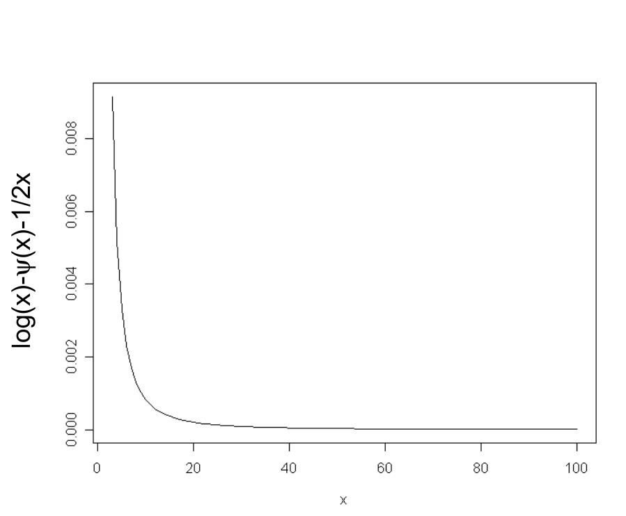
Note that function $\psi$ verifies the following asymptotic series’ expansion (1) :

	$\displaystyle\psi(x)$	$\displaystyle\underset{x\rightarrow\infty}{\sim}\ln(x)-\frac{1}{2x}-\sum_{n=1}^{\infty}\frac{B_{2n}}{2n\,x^{2n}}$
		$\displaystyle\underset{x\rightarrow\infty}{\sim}\ln(x)-\frac{1}{2x}-\frac{1}{12\,x^{2}}+\frac{1}{120\,x^{4}}+\ldots$

The convergence is very fast (see Figure 19) so that we choose to initiate Newton-Raphson algorithm with $x_{0}=\frac{1}{2C}$ .

Appendix C Computation of the moments of gamma and log gamma, beta and log beta distribution implied in the expection step

C.1 First and second moments for the sufficient statistics of the gamma pdf

Let $Z$ be a random variable with gamma distribution, $Z\sim\Gamma(s,t)$ . Using laplace transform it is easy to obtain the first moment of $\ln(Z)$ :

\mathbb{E}\left(e^{\lambda\ln(Z)}\right)=\mathbb{E}\left(Z^{\lambda}\right)=\frac{t^{s}}{\Gamma(s)}\int_{0}^{+\infty}y^{\lambda}y^{s-1}e^{-ty}dy=\frac{\Gamma(s+\lambda)}{\Gamma(s)t^{\lambda}}.

Differentiating this equation with respect to $\lambda$ , we have the expected value of $\ln(Z)$ (when $\lambda=0)$ and $Z\ln(Z)$ (when $\lambda=1)$ :

\left.\frac{\partial\mathbb{E}\left(Z^{\lambda}\right)}{\partial\lambda}\right|_{\lambda=0}=\mathbb{E}\left(\ln(Z)\right)=\psi(s)-\ln(t),

(C.1)

and

\quad\left.\frac{\partial\mathbb{E}\left(Z^{\lambda}\right)}{\partial\lambda}\right|_{\lambda=1}=\mathbb{E}\left(Z\ln(Z)\right)=\frac{s}{t}\left(\psi(s+1)-\ln(t)\right).

(C.2)

Taking the second order derivative, we show :

\left.\frac{\partial^{2}\mathbb{E}\left(Z^{\lambda}\right)}{\partial\lambda^{2}}\right|_{\lambda=0}=\mathbb{E}\left(\ln(Z)^{2}\right)=\psi^{\prime}(s)+\psi(s)^{2}-2\ln(t)\psi(s)+\ln(t)^{2}.

(C.3)

Therefore the variance-covariance matrix between $Z$ and $\ln(Z)$ is :

\left(\begin{array}[c]{cc}\frac{s}{t^{2}}&\frac{1}{t}\\ \frac{1}{t}&\psi^{\prime}(s)\end{array}\right)

C.2 First and second moments for the sufficient statistics of the beta pdf

Let $S$ be a random variable with beta distribution $S\sim\beta(s,t)$ .

\mathbb{E}\left(e^{\lambda\ln(S)}\right)=\frac{\Gamma(s+t)}{\Gamma(s+t+\lambda)}\frac{\Gamma(s+\lambda)}{\Gamma(s)}

So that, by first and second differentiation, one gets, (the derivation is quite straightfully performed if working with $\ln\mathbb{E}\left(e^{\lambda\ln(S)}\right)$ ) :

	$\displaystyle\mathbb{E}\left(\ln(S)\right)$	$\displaystyle=\psi(s)-\psi(s+t)\quad,\quad\mathbb{E}\left(\ln(1-S)\right)=\psi(t)-\psi(s+t)$
	$\displaystyle\mathbb{E}\left(\ln(S)^{2}\right)$	$\displaystyle=\psi^{\prime}(s)-\psi^{\prime}(s+t)+\left(\psi(s)-\psi(s+t)\right)^{2}$

One can extend the properties of characteristic function by considering the function of the two arguments $\lambda$ and $\mu$

\mathbb{E}\left(e^{\lambda\ln(S)+\mu\ln(1-S)}\right)=\frac{\Gamma(s+t)}{\Gamma(s+t+\lambda)}\frac{\Gamma(s+\lambda)}{\Gamma(s)}\frac{\Gamma(t+\mu)}{\Gamma(t)}

By cross-differentiation under regularity conditions (working with $\ln\mathbb{E}\left(S^{\lambda}(1-S)^{\mu}\right)$ makes things easier here also) , the joint moment can be analytically obtained :

	$\displaystyle\left.\frac{\partial^{2}\mathbb{E}\left(S^{\lambda}(1-S)^{\mu}\right)}{\partial\lambda\partial\mu}\right\|_{\lambda=0,\mu=0}$	$\displaystyle=\mathbb{E}\left(\ln(S)\ln(1-S)\right)$
		$\displaystyle=-\psi^{\prime}(s+t)+\mathbb{E}\left(\ln(S)\right)\mathbb{E}\left(\ln(1-S)\right)$

Therefore the variance-covariance matrix between $\ln(S)$ and $\ln(1-S)$ reads :

\left(\begin{array}[c]{cc}\psi^{\prime}(s)-\psi^{\prime}(s+t)&-\psi^{\prime}(s+t)\\ -\psi^{\prime}(s+t)&\psi^{\prime}(t)-\psi^{\prime}(s+t)\end{array}\right)

Appendix D EM algorithm principle

From a constructive point of view, one often writes

[x,z\left|\theta\right.]=\left[x\left|\theta,z\right.\right]\times\left[z\left|\theta\right.\right],

but using Bayes rule, we may write the reverse logarithmic form :

\ln\left[x\left|\theta\right.\right]=\ln[x,z\left|\theta\right.]-\ln\left[z\left|\theta,x\right.\right]

(D.1)

Let us remark that relation D.1 is valid whatever $z$ represents.

D.1 Recall about EM algorithm and control of the gradient

Under regularity conditions for the joint distribution $[x,z\left|\theta\right.]$ and the conditional one $\left[z\left|\theta,x\right.\right]$ , integrating relation D.1 with respect to the probability density $\left[z\left|\theta^{\prime},x\right.\right]$ :

	$\displaystyle\ln\left[x\left\|\theta\right.\right]$	$\displaystyle=\int\limits_{z}\ln[x,z\left\|\theta\right.]\left[z\left\|\theta^{\prime},x\right.\right]dz-\int\limits_{z}\ln\left[z\left\|\theta,x\right.\right]\left[z\left\|\theta^{\prime},x\right.\right]dz$
		$\displaystyle=Q(\theta,\theta^{\prime})-H(\theta,\theta^{\prime})$		(D.2)

The maximum of $\theta\mapsto H(\theta,\theta^{\prime})$ is achieved in $\theta=\theta^{\prime}$ (27).

So $H(\theta,\theta^{\prime})<H(\theta^{\prime},\theta^{\prime})$ .Let us consider D.2 for $\theta$ and $\theta^{\prime}$

\ln\left[x\left|\theta\right.\right]-\ln\left[x\left|\theta^{\prime}\right.\right]=\left(Q(\theta,\theta^{\prime})-Q(\theta^{\prime},\theta^{\prime})\right)+\left(H(\theta^{\prime},\theta^{\prime})-H(\theta,\theta^{\prime})\right)

EM algorithm is based upon an iterative procedure which exhibits $\theta$ such that $Q(\theta,\theta^{\prime})>Q(\theta^{\prime},\theta^{\prime})$ . The best $\theta$ is obtained by

\theta=\underset{\theta}{argmax\ }Q(\theta,\theta^{\prime})

During iteration we can monitor the value of the gradient for the log likelihood :

\frac{\partial\ln\left[x\left|\theta\right.\right]}{\partial\theta}=\frac{\partial\ln[x,z\left|\theta\right.]}{\partial\theta}-\frac{\partial\ln\left[z\left|\theta,x\right.\right]}{\partial\theta}

(D.3)

Integrating the right hand term with respect to conditional density $\left[z\left|\theta,x\right.\right],$ and keeping in mind that, for any sufficiently regular pdf $f(z;\theta)$ of variable $z$ with parameter $\theta$ one can write: ${\displaystyle\int\limits_{z}}\frac{\partial\ln f(z,\theta)}{\partial\theta}f(z;\theta)dz=$ $\frac{\partial}{\partial\theta}{\displaystyle\int\limits_{z}}\frac{\partial\ln f(z,\theta)}{\partial\theta}f(z;\theta)dz=0,$ we have

	$\displaystyle\frac{\partial\ln\left[x\left\|\theta\right.\right]}{\partial\theta}$	$\displaystyle={\displaystyle\int\limits_{z}}\frac{\partial\ln[x,z\left\|\theta\right.]}{\partial\theta}\left[z\left\|\theta,x\right.\right]dz-{\displaystyle\int\limits_{z}}\frac{\partial\ln\left[z\left\|\theta,x\right.\right]}{\partial\theta}\left[z\left\|\theta,x\right.\right]dz$
	$\displaystyle\frac{\partial\ln\left[x\left\|\theta\right.\right]}{\partial\theta}$	$\displaystyle={\displaystyle\int\limits_{z}}\frac{\partial\ln[x,z\left\|\theta\right.]}{\partial\theta}\left[z\left\|\theta,x\right.\right]dz$		(D.4)

We may use this equality (computed by Monte Carlo method) to perform a gradient method to obtain the maximum likelihood or just to check along the iterations that the gradient is going to zero.

D.2 Score function

From now on, let’s call $Sc(\theta,z,x)$ = $\frac{\partial\ln[x,z\left|\theta\right.]}{\partial\theta}$ the score, i.e the complete loglikelihood gradient and $Sc(\theta_{i},z,x)$ = $\frac{\partial\ln[x,z\left|\theta\right.]}{\partial\theta_{i}}$ its $i^{th}$ component. $\nabla\theta,$ equation D.4 proves that its conditional expectation (with respect to $\left[z\left|\theta,x\right.\right]$ ) is always equal to the likelihood gradient. Pushing the derivation game one step further leads to:

	$\displaystyle\frac{\partial}{\partial\theta_{j}}\left\{\frac{\partial\ln\left[x\left\|\theta\right.\right]}{\partial\theta_{i}}\right\}$	$\displaystyle={\displaystyle\int\limits_{z}}\left\{\frac{\partial Sc_{i}}{\partial\theta_{j}}\left[z\left\|\theta,x\right.\right]+Sc_{i}\frac{\partial\left[z\left\|\theta,x\right.\right]}{\partial\theta_{j}}\frac{\left[z\left\|\theta,x\right.\right]}{\left[z\left\|\theta,x\right.\right]}\right\}dz$
	$\displaystyle\frac{\partial^{2}\ln\left[x\left\|\theta\right.\right]}{\partial\theta_{i}\partial\theta_{j}}$	$\displaystyle={\displaystyle\int\limits_{z}}\left\{\frac{\partial^{2}\ln\left[x,z\left\|\theta\right.\right]}{\partial\theta_{i}\partial\theta_{j}}+Sc_{i}\left(Sc_{j}-\frac{\partial\ln\left[x\left\|\theta\right.\right]}{\partial\theta_{j}}\right)\right\}\left[z\left\|\theta,x\right.\right]dz$		(D.5)

D.3 Information matrix

To obtain the covariance matrix of the estimators at the maximum of likelihood, the empirical information matrix needs to be computed. The second order derivative is obtained by differentiating D.1:

\frac{\partial^{2}\ln\left[x\left|\theta\right.\right]}{\partial\theta_{i}\partial\theta_{j}}=\frac{\partial^{2}\ln[x,z\left|\theta\right.]}{\partial\theta_{i}\partial\theta_{j}}-\frac{\partial^{2}\ln\left[z\left|\theta,x\right.\right]}{\partial\theta_{i}\partial\theta_{j}}

(D.6)

At the maximum $\theta=\hat{\theta}$ , formula D.3 implies $\frac{\partial\ln\left[x\left|\theta\right.\right]}{\partial\theta_{jj}}=0$ so that equation D.5 takes a more friendly aspect because the score term $\frac{\partial\ln\left[x\left|\theta\right.\right]}{\partial\theta_{j}}$ in the right hand side vanishes at $\theta=\hat{\theta}$ . Equation D.6 becomes therefore much more handy because it only involves conditional expectations of first and second derivatives of the complete likelihood terms :

\frac{\partial^{2}\ln(\left[x\left|\hat{\theta}\right.\right])}{\partial\theta_{i}\partial\theta_{j}}=\int\limits_{z}\left(\frac{\partial^{2}\ln\left[x,z\left|\hat{\theta}\right.\right]}{\partial\theta_{i}\partial\theta_{j}}+\frac{\partial\ln\left[x,z\left|\hat{\theta}\right.\right]}{\partial\theta_{i}}\frac{\partial\ln\left[x,z\left|\hat{\theta}\right.\right]}{\partial\theta_{j}}\right)\left[z\left|\hat{\theta},x\right.\right]dz

(D.7)

As $\int\limits_{z}\left(\frac{\partial\ln\left[x,z\left|\hat{\theta}\right.\right]}{\partial\theta_{j}}\right)\left[z\left|\hat{\theta},x\right.\right]dz=\frac{\partial\ln\left[x\left|\hat{\theta}\right.\right]}{\partial\theta_{j}}=0,$ the second term in the right hand side of eq D.7 can be considered as the conditional variance of the gradient of the complete log-likelihood $\ln\left[x,z\left|\hat{\theta}\right.\right]$ . This expectation can be numerically computed with the same techniques to which recourse was made for the EM algorithm.

Appendix E Detailed proofs of propositions

E.1 Proof of proposition 3.1

Since we detail the computation for one particular $s$ , we will omit to mention it in order to make the reading easier. We also note respectively $\underline{y}$ , $\underline{D}$ and $\underline{N}$ the vectors of data, catching efforts and corresponding number of clumps in one stratum.
We define $J$ as

J(\underline{N},\rho,\mu)=\left[\rho,\mu,\underline{N}\left|a,b,c,d,\underline{y},\underline{D}\right.\right].

(E.1)

Then $J$ satisfies the following set of equations :

		$\displaystyle\varpropto\left[\underline{y},\rho,\mu,\underline{N}\left\|a,b,c,d,\underline{D}\right.\right]$
		$\displaystyle\varpropto\left(\prod\limits_{i=1}^{I}\left[y_{i}\left\|N_{i},\rho\right.\right]\left[N_{i}\left\|\mu,D_{i}\right.\right]\right)\left[\mu\left\|a,b\right.\right]\left[\rho\left\|c,d\right.\right]$
		$\displaystyle\varpropto\left(\prod\limits_{i=1}^{I}\left[y_{i}\left\|N_{i},\rho,\mu\right.\right]\left[N_{i}\left\|\rho,\mu\right.\right]\right)\left(\mu^{a-1}e^{-\mu b}\right)\left(\rho^{c-1}e^{-\rho d}\right)$

with the convention that $[A|B]\varpropto f(A,B)$ means that the coefficient of proportionality only depends on $B$ .

We note $I^{\star}$ the number of zero value $y$ and we reorder the vector $y$ so that the $I^{+}=I-I^{\ast}$ non zero $y_{i}$ are the first, so that $J$ may be written as :

	$\displaystyle J(\underline{N},\rho,\mu)$	$\displaystyle\varpropto\left(\prod\limits_{i=1}^{I-I^{\star}}\left(y_{i}^{N_{i}}e^{-\rho y_{i}}\frac{\rho^{N_{i}}}{\Gamma(N_{i})}\right)\left(\frac{e^{-\mu D_{i}}(\mu\,D_{i})^{N_{i}}}{\Gamma(N_{i}+1)}\right)\right)$
		$\displaystyle\hskip 28.45274pt\left(\prod\limits_{i^{\star}=I-I^{\star}+1}^{I}\delta(N_{i^{\ast}})e^{-\mu D_{i^{\star}}}\right)\left(\mu^{a-1}e^{-\mu b}\right)\left(\rho^{c-1}e^{-\rho d}\right)$

Defining $Y_{+}=\sum_{i=1}^{I}y_{i}$ , $N_{+}=\sum_{i=1}^{I}N_{i}$ and $D_{+}=\sum_{i=1}^{I}D_{i}$ , we obtain :

J(\underline{N},\rho,\mu)\varpropto\left(\prod_{i=1}^{I^{+}}\displaystyle\frac{y_{i}^{N_{i}}}{\Gamma(N_{i})\Gamma(N_{i}+1)}\right)e^{-\rho(Y_{+}+d)}\rho^{N_{+}+c-1}e^{-\mu(D_{+}+b)}\mu^{N_{+}+a-1}

Conditionally to the latent vector $\underline{N}$ , the random effects $\rho$ and $\mu$ are independent. Isolating the terms which depend on $\mu$ on one side and those depend on $\rho$ on the other, we find that

	$\displaystyle\left[\mu\|\underline{N},\theta,\underline{y},\underline{D}\right]$	$\displaystyle\sim\Gamma(a+N_{+},b+D_{+})$
	$\displaystyle\left[\rho\|\underline{N},\theta,\underline{y}\right]$	$\displaystyle\sim\Gamma(c+N_{+},d+Y_{+})$

For the expectation step we only need to compute $\mathbb{E}_{\theta}\left(\mu_{s}\mid\underline{Y_{s}}\right)$ , $\mathbb{E}_{\theta}\left(\ln(\mu_{s})\mid\underline{Y_{s}}\right)$ and the same sufficient statistics concerning $\rho$ .
Since $\mu_{s}|\underline{N_{s}},\theta,\underline{y}$ follows a gamma distribution $\Gamma(a+N_{s+},b+D_{s+})$ , the conditional expected value $\mu_{s}$ given $\underline{N_{s}}$ and $\theta=(a,b,c,d)$ is $(a+N_{s+})/(b+D_{s+})$ .
Then

\mathbb{E}_{\theta^{\prime}}\left(\mu_{s}\mid\underline{y_{s}}\right)=\mathbb{E}_{\theta^{\prime}}\left(\frac{a^{\prime}+N_{s+}}{b^{\prime}+D_{s+}}\left|\underline{y}\right.\right)=\frac{a^{\prime}+\mathbb{E}_{\theta^{\prime}}\left(N_{s+}|\underline{y_{s}}\right)}{b^{\prime}+D_{s+}}.

If $Z$ follows gamma distribution $\Gamma(s,t)$ , then $\mathbb{E}(\ln(Z))=\psi(s)-\ln(t)$ (see annex C), so that

\mathbb{E}_{\theta^{\prime}}\left(\ln(\mu_{s})\mid\underline{y_{s}}\right)=\mathbb{E}_{\theta^{\prime}}\left(\psi(a^{\prime}+N_{s+})\left|\underline{y_{s}}\right.\right)-\ln(b^{\prime}+D_{s+}).

We have respectively for $\rho_{s}$

\mathbb{E}_{\theta^{\prime}}\left(\rho_{s}\mid\underline{y_{s}}\right)=\frac{c^{\prime}+\mathbb{E}_{\theta^{\prime}}\left(N_{s+}|\underline{y_{s}}\right)}{d^{\prime}+Y_{s+}},

and

\mathbb{E}_{\theta^{\prime}}\left(\ln(\rho_{s})\mid\underline{y_{s}}\right)=\mathbb{E}_{\theta^{\prime}}\left(\psi(c^{\prime}+N_{s+})\left|\underline{y_{s}}\right.\right)-\ln(d^{\prime}+Y_{s+}).

E.2 Proof of proposition 3.2

Let us define $J$ as the distribution of $\left[\rho,\mu,\underline{N}\left|\theta^{\prime},\underline{y},\underline{D}\right.\right]$ in one particular stratum $s$ . We will write $J$ in a bottom-up perspective and consider the distribution of $\mu$ and $\rho$ conditionned by $N$ , because $\mu$ and $\rho$ are conditionally independant.

$J$ is given by :

	$\displaystyle J(\underline{N},\rho,\mu)$	$\displaystyle=\left[\rho,\mu,\underline{N}\left\|\theta^{\prime},\underline{y},\underline{D}\right.\right]$
		$\displaystyle=\left[\rho\left\|\underline{N},\theta,\underline{y}\right.\right]\left[\mu\left\|\underline{N},\theta^{\prime},\underline{y},\underline{D}\right.\right]\left[\underline{N}\left\|,\theta,\underline{y},\underline{D}\right.\right]$

Using the independent conditional gamma distributions of $\mu$ and $\rho$ and integrating according to $\mu$ and $\rho$ given $\underline{N},$ we can exhibit all the terms depending on $\underline{N}$ .

	$\displaystyle\int_{\rho}\int_{\mu}$	$\displaystyle J(\underline{N},\rho,\mu)d\mu\,d\rho=\left[\underline{N}\left\|\theta,\underline{y},\underline{D}\right.\right]$
		$\displaystyle\propto\prod_{i=1}^{I^{+}}\left(\frac{y_{i}^{N_{i}}}{\Gamma(N_{i})\Gamma(N_{i}+1)}\right)\prod_{i^{\star}=I-I^{\star+1}}^{I}\delta(N_{i^{\star}})\left(\frac{(b^{\prime}+D_{+})^{N_{+}}(d+Y_{+})^{N_{+}}}{\Gamma(a+N_{+})\Gamma(c+N_{+})}\right)^{-1}$

E.3 Proof of proposition 3.4

In the following $Z$ will stand for all the hidden variables i.e $\underline{\mathbf{Z}}=\left(\underline{\mathbf{N}},\bm{\mu},\bm{\rho}\right)$ , $\left|M_{ij}\right|$ is another notation for matrix $M$ that details the content of the $i^{th}$ row and $j^{th}$ column, and $\frac{\partial F(\theta)}{\partial\theta}$ stands for the gradient of $F$ written as a vector whose $i^{th}$ component is the scalar $\frac{\partial F(\theta)}{\partial\theta_{i}}$ . The key equation involves rewriting equation D.7 as the expectation of the second order derivative of the complete log-likelihood and the variance of the score (its gradient) to be taken with regards to the conditional distribution $\left[Z\left|x,\hat{\theta}\right.\right]$ (see annex D.3)

\left|\frac{\partial^{2}\ln(\left[x\left|\hat{\theta}\right.\right])}{\partial\theta_{i}\partial\theta_{j}}\right|=\mathbb{E}_{Z|x}\left|\frac{\partial^{2}\ln(\left[x,Z\left|\hat{\theta}\right.\right])}{\partial\theta_{i}\partial\theta_{j}}\right|+\mathbb{V}ar_{Z|x}\left(\frac{\partial\ln\left[x,Z\left|\theta\right.\right]}{\partial\theta}\right)

(E.2)

Computing the first term of the right hand side of equation E.2 is easy, since $\left[x\left|z,\theta\right.\right]=\left[x\left|z\right.\right]$ (consequently the complete log-likelihood $\ln(\left[x,z\left|\theta\right.\right])$ can be separated as $\ln(\left[x\left|z\right.\right])+\ln(\left[z,\left|\theta\right.\right])$ ) and the gamma random effects $\left[z|\theta\right]$ belong to an exponential family. As a consequence, annex F shows that

\mathbb{E}\left|\frac{\partial^{2}\ln(\left[x,Z\left|\hat{\theta}\right.\right])}{\partial\theta_{i}\partial\theta_{j}}\right|=\left|\frac{\partial^{2}\ln(\left[x,z\left|\hat{\theta}\right.\right])}{\partial\theta_{i}\partial\theta_{j}}\right|=S\,\left(\begin{array}[c]{cccc}-\psi^{\prime}(\hat{a})&\frac{1}{\hat{b}}&0&0\\ \frac{1}{b}&-\frac{\hat{a}}{\hat{b}^{2}}&0&0\\ 0&0&-\psi^{\prime}(\hat{c})&\frac{1}{\hat{d}}\\ 0&0&\frac{1}{\hat{d}}&\frac{-\hat{c}}{\hat{d}^{2}}\end{array}\right)

As shown in Figure 20. , given $Y_{s},Y_{s^{\prime}}$ and $\theta,$ the latent variables $Z_{s}$ and $Z_{s^{\prime}}$ of two stratum $s$ and $s^{\prime}$ are conditionnaly independent, therefore :

\mathbb{V}ar_{Z|x}\left(\frac{\partial\ln\left[x,Z\left|\theta\right.\right]}{\partial\theta}\right)=\sum_{s=1}^{S}\mathbb{V}ar_{Z_{s}|x}\left(\begin{array}[c]{c}\ln(\mu_{s})\\ -\mu_{s}\\ \ln(\rho_{s})\\ -\rho_{s}\end{array}\right)

To evaluate the variance of the score in stratum s, we will take advantage of successive conditioning due to the hierarchical structure depicted in Figure 2. Recalling that the latent variable $Z_{s}$ includes, in addition to $(\mu_{s},\rho_{s})$ , the vector $\underline{N_{s}}$ , i-e the latent number of clumps for each record, the variance conditional decomposition formula gives:

\mathbb{V}ar_{Z_{s}|x}\left(\begin{array}[c]{c}\ln(\mu_{s})\\ -\mu_{s}\\ \ln(\rho_{s})\\ -\rho_{s}\end{array}\right)=\mathbb{E}_{\underline{N_{s}}|x}\left(\mathbb{V}ar\left(\begin{array}[c]{c}\ln(\mu_{s})\\ -\mu_{s}\\ \ln(\rho_{s})\\ -\rho_{s}\end{array}|\underline{N_{s}}\right)\right)+\mathbb{V}ar_{\underline{N_{s}}|x}\left(\mathbb{E}\left(\begin{array}[c]{c}\ln(\mu_{s})\\ -\mu_{s}\\ \ln(\rho_{s})\\ -\rho_{s}\end{array}|\underline{N_{s}}\right)\right)

So that we have

I_{e}(\hat{\theta},x)=S\,\left(\begin{matrix}-\psi^{\prime}(\hat{a})&\frac{1}{\hat{b}}&0&0\\ \frac{1}{\hat{b}}&-\frac{\hat{a}}{\hat{b}^{2}}&0&0\\ 0&0&-\psi^{\prime}(\hat{c})&\frac{1}{\hat{d}}\\ 0&0&\frac{1}{\hat{d}}&-\frac{\hat{c}}{\hat{d}^{2}}\\ &&&\end{matrix}\right)+\sum_{s=1}^{S}(A_{s}+B_{s})

with

A_{s}=\mathbb{E}_{\underline{\mathbf{N}}|x}\left(\mathbb{V}ar\left(\begin{array}[c]{c}\ln(\mu_{s})\\ -\mu_{s}\\ \ln(\rho_{s})\\ -\rho_{s}\end{array}|\underline{\mathbf{N}}\right)\right)\quad\mbox{and}\quad B_{s}=\mathbb{V}ar_{\underline{N_{s}}|x}\left(\mathbb{E}\left(\begin{array}[c]{c}\ln(\mu_{s})\\ -\mu_{s}\\ \ln(\rho_{s})\\ -\rho_{s}\end{array}|\underline{N_{s}}\right)\right).

Given $\underline{N_{s}}$ , $\mu_{s}$ and $\rho_{s}$ are independent. Moreover the pdf $[\rho_{s}|\underline{N_{s}},\underline{Y_{s}},a,b,c,d]$ and $[\mu_{s}|\underline{N_{s}},\underline{Y_{s}},a,b,c,d]$ are gamma and analytic expressions are available for the expectation and variance of the gamma sufficient statistics, as detailed in equations C.1 to C.3. The key functions of $N_{s+}$ are ( $a_{s}\prime,b_{s}\prime,c_{s}\prime,d_{s}\prime)=(a+N_{s+},b+D_{s+},c+N_{s+},d+Y_{s+})$ such that :

\mathbb{E}\left(\begin{array}[c]{c}\ln(\mu_{s})\\ -\mu_{s}\\ \ln(\rho_{s})\\ -\rho_{s}\end{array}|\underline{\mathbf{N}}\right)=\left(\begin{array}[c]{c}\psi(a_{s}^{\prime})-\ln(b_{s}^{\prime})\\ -\frac{a_{s}^{\prime}}{b_{s}^{\prime}}\\ \psi(c_{s}^{\prime})-\ln(d_{s}^{\prime})\\ -\frac{c_{s}^{\prime}}{d_{s}^{\prime}}\end{array}\right)

and then $B_{s}$ is obtained by taking the covariance of this vector :

B_{s}=\mathbb{V}ar_{N_{s+}|\hat{\theta},x}\left(\mathbb{E}\left(\begin{array}[c]{c}\ln(\mu_{s})\\ -\mu_{s}\\ \ln(\rho_{s})\\ -\rho_{s}\end{array}|\underline{\mathbf{N_{s+}}}\right)\right)

Given $\underline{N_{s}}$ additional advantage is taken from the conditional independence of $\rho_{s}$ and $\mu_{s}$ as shown in Figure 21, .

\mathbb{V}ar\left(\begin{array}[c]{c}\ln(\mu_{s})\\ -\mu_{s}\\ \ln(\rho_{s})\\ -\rho_{s}\end{array}|\underline{\mathbf{N}}\right)=\left(\begin{array}[c]{cccc}-\psi^{\prime}(a^{\prime})&\frac{1}{b^{\prime}}&0&0\\ \frac{1}{b^{\prime}}&-\frac{a^{\prime}}{b^{\prime 2}}&0&0\\ 0&0&-\psi^{\prime}(c^{\prime})&\frac{1}{d^{\prime}}\\ 0&0&\frac{1}{d^{\prime}}&\frac{-c^{\prime}}{d^{\prime 2}}\end{array}\right)

and the expression for $A_{s}$ follows easily.

Appendix F Second derivative of the complete log-likelihood

Let us first recall the complete log likelihood of the model :

	$\displaystyle\ln\left[x,z\left\|\theta\right.\right]$	$\displaystyle=C_{-\theta}+(a-1)\sum\limits_{s=1}^{S}\ln\mu_{s}+Sa\ln b-b\sum\limits_{s=1}^{S}\mu_{s}-S\ln\Gamma(a)$
		$\displaystyle+(c-1)\sum\limits_{s=1}^{S}\ln\rho_{s}+Sc\ln d-d\sum\limits_{s=1}^{S}\rho_{s}-S\ln\Gamma(c)$

In the first derivative, the latent variables $\bm{\mu}$ and $\bm{\rho}$ appear not surprisingly only through their arithmetic or geometric means (sufficient statistics for the gamma pdf). Using standard notation $\bar{\mu}$ for the arithmetic mean $\frac{1}{S}\sum_{s=1}^{S}\mu_{s}$ , we have :

	$\displaystyle\frac{\partial\ln\left[x,z\left\|\theta\right.\right]}{\partial a}=S\left(\overline{\ln(\mu)}+\ln b-\psi(a)\right)$	$\displaystyle\qquad\frac{\partial\ln\left[x,z\left\|\theta\right.\right]}{\partial c}=S\left(\overline{\ln(\rho)}+\ln d-\psi(c)\right)$
	$\displaystyle\frac{\partial\ln\left[x,z\left\|\theta\right.\right]}{\partial b}=S\left(\frac{a}{b}-\overline{\mu}\right)$	$\displaystyle\qquad\frac{\partial\ln\left[x,z\left\|\theta\right.\right]}{\partial d}=S\left(\frac{c}{d}-\overline{\rho}\right)$

The gradient of the complete log-likelihood (so-called the ”score”) may be split into two parts : the first one $\Delta_{\theta}$ does not depend on the latent variable $z$ while the other one $\Delta_{z}$ gathers terms depending on $z$ (and possibly of $\theta$ ), i.e :

\left(\frac{\partial\ln\left[x,z\left|\hat{\theta}\right.\right]}{\partial\theta}\right)=\Delta_{\theta}+\Delta_{z}

with

\begin{array}[c]{cc}\Delta_{\theta}=S\left(\begin{array}[c]{c}\ln b-\psi(a)\\ \frac{a}{b}\\ \ln d-\psi(c)\\ \frac{c}{d}\end{array}\right)&\Delta_{z}=S\left(\begin{array}[c]{c}\overline{\ln(\mu)}\\ -\overline{\mu}\\ \overline{\ln(\rho)}\\ -\overline{\rho}\end{array}\right)\end{array}

In addition here, $\Delta_{z}$ does not contain terms with $\theta$ , consequently the second order derivatives are easy to obtain and don’t involve the latent variable :

	$\displaystyle\frac{\partial^{2}\ln\left[x,z\left\|\theta\right.\right]}{\partial a\partial a}=-S\psi^{\prime}(a)$	$\displaystyle\quad\frac{\partial^{2}\ln\left[x,z\left\|\theta\right.\right]}{\partial c\partial c}=-S\psi^{\prime}(c)$
	$\displaystyle\frac{\partial^{2}\ln\left[x,z\left\|\theta\right.\right]}{\partial a\partial b}=\frac{S}{b}$	$\displaystyle\quad\frac{\partial^{2}\ln\left[x,z\left\|\theta\right.\right]}{\partial c\partial d}=\frac{S}{d}$
	$\displaystyle\frac{\partial^{2}\ln\left[x,z\left\|\theta\right.\right]}{\partial b\partial b}=-\frac{Sa}{b^{2}}$	$\displaystyle\quad\frac{\partial^{2}\ln\left[x,z\left\|\theta\right.\right]}{\partial d\partial d}=\frac{-Sc}{d^{2}}$

Appendix G Second derivative of the complete log-likelihood with discrete data

The complete log likelihood of the model, in the discrete case, reads :

	$\displaystyle\ln\left[x,z\left\|\theta\right.\right]$	$\displaystyle=C_{-\theta}+(a-1)\sum\limits_{s=1}^{S}\ln\mu_{s}+Sa\ln b-b\sum\limits_{s=1}^{S}\mu_{s}-S\ln\Gamma(a)$
	$\displaystyle S\ln\left(\frac{\Gamma(c+d)}{\Gamma(c)\Gamma(d)}\right)$	$\displaystyle+(c-1)\sum\limits_{s=1}^{S}\ln p_{s}+(d-1)\sum\limits_{s=1}^{S}\ln(1-p_{s})$

In the first derivative, the latent variables $\bm{\mu}$ and $\bm{p}$ appear only through their arithmetic or geometric means (sufficient statistics for the gamma and beta pdf). Using standard notation $\bar{\mu}$ for the arithmetic mean $\frac{1}{S}\sum_{s=1}^{S}\mu_{s}$ , we have :

	$\displaystyle\frac{\partial\ln\left[x,z\left\|\theta\right.\right]}{\partial a}=S\left(\overline{\ln(\mu)}+\ln b-\psi(a)\right)$	$\displaystyle\qquad\frac{\partial\ln\left[x,z\left\|\theta\right.\right]}{\partial c}=S\left(\overline{\ln(p)}+\psi(c+d)-\psi(c)\right)$
	$\displaystyle\frac{\partial\ln\left[x,z\left\|\theta\right.\right]}{\partial b}=S\left(\frac{a}{b}-\overline{\mu}\right)$	$\displaystyle\qquad\frac{\partial\ln\left[x,z\left\|\theta\right.\right]}{\partial d}=S\left(\overline{\ln(1-p)}+\psi(c+d)-\psi(d)\right)$

\left(\frac{\partial\ln\left[x,z\left|\hat{\theta}\right.\right]}{\partial\theta}\right)=\Delta_{\theta}+\Delta_{z}

with

\begin{array}[c]{cc}\Delta_{\theta}=S\left(\begin{array}[c]{c}\ln b-\psi(a)\\ \frac{a}{b}\\ \psi(c+d)-\psi(c)\\ \psi(c+d)-\psi(d)\end{array}\right)&\Delta_{z}=S\left(\begin{array}[c]{c}\overline{\ln(\mu)}\\ -\overline{\mu}\\ \overline{\ln(p)}\\ \overline{\ln(1-p)}\end{array}\right)\end{array}

In addition here, $\Delta_{z}$ does not contain terms with $\theta$ , consequently the second order derivatives are easy to obtain and don’t involve the latent variable; with $Z$ standing for all the hidden variables i.e $\underline{\mathbf{Z}}=\left(\underline{\mathbf{N}},\bm{\mu},\bm{p}\right)$ :

\left|\frac{\partial^{2}\ln(\left[x,z\left|\hat{\theta}\right.\right])}{\partial\theta_{i}\partial\theta_{j}}\right|=S\,\left(\begin{array}[c]{cccc}-\psi^{\prime}(\hat{a})&\frac{1}{\hat{b}}&0&0\\ \frac{1}{b}&-\frac{\hat{a}}{\hat{b}^{2}}&0&0\\ 0&0&-\psi^{\prime}(\hat{c})+\psi^{\prime}(\hat{c}+\hat{d})&\psi^{\prime}(\hat{c}+\hat{d})\\ 0&0&\psi^{\prime}(\hat{c}+\hat{d})&-\psi^{\prime}(\hat{d})+\psi^{\prime}(\hat{c}+\hat{d})\end{array}\right)

As shown in Figure 20 for the continuous case , given $Y_{s},Y_{s^{\prime}}$ and $\theta,$ the latent variables $Z_{s}$ and $Z_{s^{\prime}}$ of two strata $s$ and $s^{\prime}$ are conditionnaly independent, therefore :

\mathbb{V}ar_{Z|x}\left(\frac{\partial\ln\left[x,Z\left|\theta\right.\right]}{\partial\theta}\right)=\sum_{s=1}^{S}\mathbb{V}ar_{Z_{s}|x}\left(\begin{array}[c]{c}\ln(\mu_{s})\\ -\mu_{s}\\ \ln(p_{s})\\ \ln(1-p_{s})\end{array}\right)

To evaluate the variance of the score in stratum s, we will take advantage from successive conditioning due to the hierarchical structure depicted in Figure 2 still true for the discrete case. The variance conditional decomposition formula gives:

\mathbb{V}ar_{Z_{s}|x}\left(\begin{array}[c]{c}\ln(\mu_{s})\\ -\mu_{s}\\ \ln(\rho_{s})\\ -\rho_{s}\end{array}\right)=\mathbb{E}_{\underline{N_{s}}|x}\left(\mathbb{V}ar\left(\begin{array}[c]{c}\ln(\mu_{s})\\ -\mu_{s}\\ \ln(p_{s})\\ \ln(1-p_{s})\end{array}|\underline{N_{s}}\right)\right)+\mathbb{V}ar_{\underline{N_{s}}|x}\left(\mathbb{E}\left(\begin{array}[c]{c}\ln(\mu_{s})\\ -\mu_{s}\\ \ln(p_{s})\\ \ln(1-p_{s})\end{array}|\underline{N_{s}}\right)\right)

So that we have

I_{e}(\hat{\theta},x)=S\,\left(\begin{array}[c]{cccc}-\psi^{\prime}(\hat{a})&\frac{1}{\hat{b}}&0&0\\ \frac{1}{b}&-\frac{\hat{a}}{\hat{b}^{2}}&0&0\\ 0&0&-\psi^{\prime}(\hat{c})+\psi^{\prime}(\hat{c}+\hat{d})&\psi^{\prime}(\hat{c}+\hat{d})\\ 0&0&\psi^{\prime}(\hat{c}+\hat{d})&-\psi^{\prime}(\hat{d})+\psi^{\prime}(\hat{c}+\hat{d})\end{array}\right)+\sum_{s=1}^{S}(A_{s}+B_{s})

with

A_{s}=\mathbb{E}_{\underline{\mathbf{N}}|x}\left(\mathbb{V}ar\left(\begin{array}[c]{c}\ln(\mu_{s})\\ -\mu_{s}\\ \ln(p_{s})\\ \ln(1-p_{s})\end{array}|\underline{\mathbf{N}}\right)\right)\quad\mbox{and}\quad B_{s}=\mathbb{V}ar_{\underline{N_{s}}|x}\left(\mathbb{E}\left(\begin{array}[c]{c}\ln(\mu_{s})\\ -\mu_{s}\\ \ln(p_{s})\\ \ln(1-p_{s})\end{array}|\underline{N_{s}}\right)\right).

Given $\underline{N_{s}}$ , $\mu_{s}$ and $\rho_{s}$ are independent. Moreover the pdf $[\rho_{s}|\underline{N_{s}},\underline{Y_{s}},a,b,c,d]$ and $[p_{s}|\underline{N_{s}},\underline{Y_{s}},a,b,c,d]$ are gamma and beta so that analytic expressions are available for the expectation and variance of the gamma sufficient statistics, as detailed in equations C.1 to C.3. The key functions of $N_{s+}$ are ( $a_{s}\prime,b_{s}\prime,c_{s}\prime,d_{s}\prime)=(a+N_{s+},b+D_{s+},c+N_{s+},d+Y_{s+}-N_{s+})$ such that :

\mathbb{E}\left(\begin{array}[c]{c}\ln(\mu_{s})\\ -\mu_{s}\\ \ln(p_{s})\\ \ln(1-p_{s})\end{array}|\underline{\mathbf{N}}\right)=\left(\begin{array}[c]{c}\psi(a_{s}^{\prime})-\ln(b_{s}^{\prime})\\ -\frac{a_{s}^{\prime}}{b_{s}^{\prime}}\\ \psi(c_{s}^{\prime})-\psi(c_{s}^{\prime}+d_{s}^{\prime})\\ \psi(d_{s}^{\prime})-\psi(c_{s}^{\prime}+d_{s}^{\prime})\end{array}\right)

and then the matrix $B_{s}$ is obtained by taking the covariance of this vector.Given $\underline{N_{s}}$ additional advantage is taken from the conditional independence of $p_{s}$ and $\mu_{s}$ (as shown on Figure 21 for the continuous case).

\mathbb{V}ar\left(\begin{array}[c]{c}\ln(\mu_{s})\\ -\mu_{s}\\ \ln(\rho_{s})\\ -\rho_{s}\end{array}|\underline{\mathbf{N}}\right)=\left(\begin{array}[c]{cccc}-\psi^{\prime}(a^{\prime})&\frac{1}{b^{\prime}}&0&0\\ \frac{1}{b^{\prime}}&-\frac{a^{\prime}}{b^{\prime 2}}&0&0\\ 0&0&\psi^{\prime}(c_{s}^{\prime})-\psi^{\prime}(c_{s}^{\prime}+d_{s}^{\prime})&-\psi^{\prime}(c_{s}^{\prime}+d_{s}^{\prime})\\ 0&0&-\psi^{\prime}(c_{s}^{\prime}+d_{s}^{\prime})&\psi^{\prime}(d_{s}^{\prime})-\psi^{\prime}(c_{s}^{\prime}+d_{s}^{\prime})\end{array}\right)

and the expectation to obtain $A_{s}$ is performed via importance sampling.

To sum it up

I_{e}(\theta)=-\frac{\partial^{2}\ln{[\underline{\mathbf{Y}}|\theta]}}{\partial\theta_{i}\,\partial\theta_{j}}

(G.1)

At the maximum likelihood estimator $\hat{\theta}$ , the following equality occurs :

I_{e}(\hat{\theta},\underline{\mathbf{Y}})=S\,\left(\begin{array}[c]{cccc}-\psi^{\prime}(\hat{a})&\frac{1}{\hat{b}}&0&0\\ \frac{1}{b}&-\frac{\hat{a}}{\hat{b}^{2}}&0&0\\ 0&0&-\psi^{\prime}(\hat{c})+\psi^{\prime}(\hat{c}+\hat{d})&\psi^{\prime}(\hat{c}+\hat{d})\\ 0&0&\psi^{\prime}(\hat{c}+\hat{d})&-\psi^{\prime}(\hat{d})+\psi^{\prime}(\hat{c}+\hat{d})\end{array}\right)+\sum_{s=1}^{S}(A_{s}+B_{s})

(G.2)

with

A_{s}=\left(\begin{matrix}\mathbb{E}_{\nu_{s}}(\psi^{\prime}(a_{s}^{\prime}))&\frac{-1}{b_{s}^{\prime}}&0&0\\ \frac{-1}{b_{s}^{\prime}}&\frac{\mathbb{E}_{N_{s+}|\underline{\mathbf{Y}},\hat{\theta}}(a_{s}^{\prime})}{b_{s}^{\prime}{}^{2}}&0&0\\ 0&0&\mathbb{E}_{\nu_{s}}(\psi^{\prime}(c_{s}^{\prime})-\psi^{\prime}(c_{s}^{\prime}+d_{s}^{\prime}))&-\mathbb{E}_{\nu_{s}}(\psi^{\prime}(c_{s}^{\prime}+d_{s}^{\prime}))\\ 0&0&-\mathbb{E}_{\nu_{s}}(\psi^{\prime}(c_{s}^{\prime}+d_{s}^{\prime}))&\mathbb{E}_{\nu_{s}}(\psi^{\prime}(d_{s}^{\prime})-\psi^{\prime}(c_{s}^{\prime}+d_{s}^{\prime}))\end{matrix}\right)

and

B_{s}=\mathbb{V}ar_{N_{s+}|\hat{\theta},x}\left(\begin{array}[c]{c}\psi(a_{s}^{\prime})-\ln(b_{s}^{\prime})\\ -\frac{a_{s}^{\prime}}{b_{s}^{\prime}}\\ \psi(c_{s}^{\prime})-\psi(c_{s}^{\prime}+d_{s}^{\prime})\\ \psi(d_{s}^{\prime})-\psi(c_{s}^{\prime}+d_{s}^{\prime})\end{array}\right)

where $a_{s}^{\prime}=\hat{a}+N_{s+}$ , $b_{s}^{\prime}=\hat{b}+D_{s+}$ , $c^{\prime}=\hat{c}+N_{s+}$ and $d_{s}^{\prime}=\hat{d}+Y_{s+}-N_{s+}$ ( $b_{s}^{\prime}$ is the only term that is not a function of $N_{s+}$ , thus behaving like a constant with regards to the $\mathbb{V}ar_{N_{s+}|\hat{\theta},x}$ operator)

Appendix H The discrete algorithm

If we adapt bluntly from the continuous version, the algoritm would write

1.

Generate $N_{i}^{(g)}=0$ wherever $y_{i=0}$ for $i=I-I^{+}+1,\ldots,I$ .

Generate a value of $N_{+}$ according to

N_{+}\varpropto\frac{\Gamma(a^{\prime}+N_{+})\Gamma(c^{\prime}+N_{+})\Gamma(d^{\prime}+Y_{+}-N_{+})D_{+}^{N_{+}}}{(b^{\prime}+D_{+})^{a^{\prime}+N_{+}}\prod_{j=1}^{I^{+}}\Gamma\left(N_{+}\frac{Y_{j}D_{j}}{(YD)_{+}}\right)}

Generate each $N_{i}$ for $i=1,\ldots,I^{+}$ , so that the vector $\underline{N}$ is distributed according to a multivariate hypegeometric Fisher distribution (17) given by

[\underline{N}|N_{+}]=\frac{g(\underline{N};N_{+},\underline{Y},\underline{D}/D_{+})}{K_{N_{+}}}

with

g(\underline{N};N_{+},\underline{Y},\underline{D})=\prod_{i=I^{*}+1}^{I}\left(\begin{array}[]{c}Y_{j}\cr N_{j}\end{array}\right)(D_{j}/D_{+})^{N_{j}},

K_{N_{+}}=\sum_{y\in\mathcal{S}}g(\underline{y};N_{+},\underline{Y},\underline{D}),

and

\mathcal{S}=\left\{\underline{N}\in\mathbb{Z}^{I^{+}}_{+}|\sum_{i=I^{*}+1}^{I}N_{i}=N_{+}\right\}.

4.

Associate to the vector the weight

$w^{(g)}=K_{N^{(g)}_{+}}\prod_{i=I^{*}}^{I}\frac{\Gamma\left(N^{(g)}_{+}\frac{Y_{j}D_{j}}{(YD)_{+}}\right)}{\Gamma(N_{j})}.$

Importance Sampling relying this time on the multivariate hypergeometric distribution seems to stand naturally as the core of the algorithm to evaluate (3.23). But during our first trials, the above adaptation of the continuous version performed very badly, leading to a large variance of the importance weights, i.e. a degeneracy phenomenon that would put the all weight onto a very few contributing particles. In order to put more weight onto particles that have a good chance to efficiently attain the target distribution, a mixture was chosen as the importance distribution for a modified algorithm. The idea is similar in spirit to the auxiliary particle filtering of [20]. More precisely, the first step consists of determining an approximate mean of $N_{s+}$ in stratum $s$ , denoted $N_{s+}^{(ref)}$ . One draws a L-sample of $N_{s+}$ according to

g(N_{+})\varpropto\frac{\Gamma(a^{\prime}+N_{+})\Gamma(c^{\prime}+N_{+})\Gamma(d^{\prime}+y_{+}-N_{+})D_{+}^{N_{+}}}{\Gamma(b^{\prime}+D_{+})^{a^{\prime}+N_{+}}\Gamma(N_{+}+1)\Gamma(N_{+})\Gamma(Y_{+}-N_{+}+1)}

The $g$ distribution corresponds to the conditional distribution of $\ N_{+}$ given the sum of the data collected in stratum $s$ but ignoring the individual records. $N_{s+}^{(ref)}$ is given by the mean over a sample that is

N_{s+}^{(ref)}=\frac{1}{L}\sum N_{+}^{(i)}

and provides a good estimation of the location of $N_{s+}$ . As previously we omit the index $s$ to make the reading easier. Subsequently, the following algorithm relies on independent but non identically distributed simulations :

1.

Generate $N_{i}^{(g)}=0$ wherever $y_{i}=0$ for $i=I-I^{+}+1,\ldots,I$ .
2.

Draw $\mu^{(g)}\sim\Gamma(a^{\prime}+N_{+}^{(ref)},b^{\prime}+D_{+})$ and $p^{(g)}\sim\beta(c^{\prime}+N_{s+}^{(ref)},d^{\prime}+Y_{s+}-N_{s+}^{(ref)})$

Given $\mu^{(g)}$ and $\rho^{(g)}$ , draw $N_{sk}^{(g)}\sim[N_{sk}|\mu^{(g)},p^{(g)},y_{sk}]$ that is :

[N_{i}^{(g)}=k]=K_{i}\left(\frac{\mu^{(g)}p^{(g)}D_{i}}{1-p^{(g)}}\right)^{N_{i}}\frac{1}{\Gamma(N_{i})\Gamma(Y_{i}-N_{i}+1)\Gamma(N_{i}+1)}\mathds{1}_{\left\{0<N_{sk}\leq Y_{si}\right\}},

where $K_{i}$ denotes the normalizing constant.

Compute the weight of each particle $g$ using

w^{(g)}=\prod_{i=1}^{I^{+}}\frac{\Gamma(N_{i}+1)}{K_{i}(\mu^{(g)}p^{(g)})^{N_{i}}}\left(\frac{\Gamma(a^{\prime}+N_{s+})\Gamma(N_{s+}+c^{\prime})\Gamma(Y_{+}-N_{s+}+d^{\prime})}{(b^{\prime}+D_{s+})^{N_{s+}}}\right)

	$\displaystyle\frac{\partial\ln\left[x\left\|\theta\right.\right]}{\partial\theta}$	$\displaystyle={\displaystyle\int\limits_{z}}\frac{\partial\ln[x,z\left\|\theta\right.]}{\partial\theta}\left[z\left\|\theta,x\right.\right]dz-{\displaystyle\int\limits_{z}}\frac{\partial\ln\left[z\left\|\theta,x\right.\right]}{\partial\theta}\left[z\left\|\theta,x\right.\right]dz$
	$\displaystyle\frac{\partial\ln\left[x\left\|\theta\right.\right]}{\partial\theta}$	$\displaystyle={\displaystyle\int\limits_{z}}\frac{\partial\ln[x,z\left\|\theta\right.]}{\partial\theta}\left[z\left\|\theta,x\right.\right]dz$		(D.4)

	$\displaystyle\frac{\partial}{\partial\theta_{j}}\left\{\frac{\partial\ln\left[x\left\|\theta\right.\right]}{\partial\theta_{i}}\right\}$	$\displaystyle={\displaystyle\int\limits_{z}}\left\{\frac{\partial Sc_{i}}{\partial\theta_{j}}\left[z\left\|\theta,x\right.\right]+Sc_{i}\frac{\partial\left[z\left\|\theta,x\right.\right]}{\partial\theta_{j}}\frac{\left[z\left\|\theta,x\right.\right]}{\left[z\left\|\theta,x\right.\right]}\right\}dz$
	$\displaystyle\frac{\partial^{2}\ln\left[x\left\|\theta\right.\right]}{\partial\theta_{i}\partial\theta_{j}}$	$\displaystyle={\displaystyle\int\limits_{z}}\left\{\frac{\partial^{2}\ln\left[x,z\left\|\theta\right.\right]}{\partial\theta_{i}\partial\theta_{j}}+Sc_{i}\left(Sc_{j}-\frac{\partial\ln\left[x\left\|\theta\right.\right]}{\partial\theta_{j}}\right)\right\}\left[z\left\|\theta,x\right.\right]dz$		(D.5)

	$\displaystyle\frac{\partial\ln\left[x,z\left\|\theta\right.\right]}{\partial a}=S\left(\overline{\ln(\mu)}+\ln b-\psi(a)\right)$	$\displaystyle\qquad\frac{\partial\ln\left[x,z\left\|\theta\right.\right]}{\partial c}=S\left(\overline{\ln(\rho)}+\ln d-\psi(c)\right)$
	$\displaystyle\frac{\partial\ln\left[x,z\left\|\theta\right.\right]}{\partial b}=S\left(\frac{a}{b}-\overline{\mu}\right)$	$\displaystyle\qquad\frac{\partial\ln\left[x,z\left\|\theta\right.\right]}{\partial d}=S\left(\frac{c}{d}-\overline{\rho}\right)$

	$\displaystyle\frac{\partial^{2}\ln\left[x,z\left\|\theta\right.\right]}{\partial a\partial a}=-S\psi^{\prime}(a)$	$\displaystyle\quad\frac{\partial^{2}\ln\left[x,z\left\|\theta\right.\right]}{\partial c\partial c}=-S\psi^{\prime}(c)$
	$\displaystyle\frac{\partial^{2}\ln\left[x,z\left\|\theta\right.\right]}{\partial a\partial b}=\frac{S}{b}$	$\displaystyle\quad\frac{\partial^{2}\ln\left[x,z\left\|\theta\right.\right]}{\partial c\partial d}=\frac{S}{d}$
	$\displaystyle\frac{\partial^{2}\ln\left[x,z\left\|\theta\right.\right]}{\partial b\partial b}=-\frac{Sa}{b^{2}}$	$\displaystyle\quad\frac{\partial^{2}\ln\left[x,z\left\|\theta\right.\right]}{\partial d\partial d}=\frac{-Sc}{d^{2}}$

	$\displaystyle\frac{\partial\ln\left[x,z\left\|\theta\right.\right]}{\partial a}=S\left(\overline{\ln(\mu)}+\ln b-\psi(a)\right)$	$\displaystyle\qquad\frac{\partial\ln\left[x,z\left\|\theta\right.\right]}{\partial c}=S\left(\overline{\ln(p)}+\psi(c+d)-\psi(c)\right)$
	$\displaystyle\frac{\partial\ln\left[x,z\left\|\theta\right.\right]}{\partial b}=S\left(\frac{a}{b}-\overline{\mu}\right)$	$\displaystyle\qquad\frac{\partial\ln\left[x,z\left\|\theta\right.\right]}{\partial d}=S\left(\overline{\ln(1-p)}+\psi(c+d)-\psi(d)\right)$

Random effects compound Poisson model to represent data with extra zeros

Abstract

Keywords:

2008 MSC

1 Introduction

2 Model construction

2.1 Compound Poisson process to introduce extra zeros

2.2 Choice of the random component XX for continuous data

2.3 Random effects

2.4 Compound Poisson process for count data

3 Estimation via the EM algorithm with importance sampling

3.1 Implementation of the MCEM algorithm

3.1.1 Maximization step

3.1.2 Expectation step by conditioning onto the number of clumps

Proposition 3.1.

Proposition 3.2.

Proposition 3.3 (Generate one particle in one particular stratum ss according to distribution 3.13).

3.1.3 Empirical Variance Matrix

Proposition 3.4.

3.1.4 Prediction of the random effects

3.2 MCEM algorithm for RDLOL model

3.2.1 Straightforward transposition to the discrete case

Proposition 3.5.

3.2.2 The covariance matrix in the discrete case

3.2.3 Prediction of the random effects

4 Applications

4.1 Real dataset - Gulf of St.Lawrence survey

4.1.1 Maximum likelihood point estimation

4.1.2 Confidence intervals

4.1.3 Validation of the gamma assumption for random effects

4.2 Simulations Studies

4.2.1 Simulation design

4.2.2 RLOL Results

5 Conclusion and Perspectives

References

Appendix A Compound Poisson process characteristic function

Appendix B Initialization of the Newton-Raphson algorithm

Appendix C Computation of the moments of gamma and log gamma, beta and log beta distribution implied in the expection step

C.1 First and second moments for the sufficient statistics of the gamma pdf

C.2 First and second moments for the sufficient statistics of the beta pdf

Appendix D EM algorithm principle

D.1 Recall about EM algorithm and control of the gradient

D.2 Score function

D.3 Information matrix

Appendix E Detailed proofs of propositions

E.1 Proof of proposition 3.1

E.2 Proof of proposition 3.2

E.3 Proof of proposition 3.4

Appendix F Second derivative of the complete log-likelihood

Appendix G Second derivative of the complete log-likelihood with discrete data

Appendix H The discrete algorithm

2.2 Choice of the random component $X$ for continuous data

Proposition 3.3 (Generate one particle in one particular stratum $s$ according to distribution 3.13).