跳到论文正文
W Papers独立论文阅读器 arXiv:0907.4872 论文正文 计算阅读时间 · 0%
引用这篇论文根据当前论文元数据生成,正式投稿前建议核对。


License: arXiv.org perpetual non-exclusive license
arXiv:0907.4872v2 [math.DS] 01 Sep 2010

Fractal tiles associated with shift radix systemsThanks: This research was supported by the Austrian Science Foundation (FWF), project S9610, which is part of the national research network FWF–S96 “Analytic combinatorics and probabilistic number theory”, by the Agence Nationale de la Recherche, grant ANR–06–JCJC-0073 “DyCoNum”, by the “Amadée” grant FR–13–2008 and the “PHC Amadeus” grant 17111UB

Valérie Berthé Address: LIRMM, CNRS UMR 5506, Université Montpellier II, 161 rue Ada, 34392 Montpellier Cedex 5, FRANCE Email address: berthe@lirmm.fr , Anne Siegel Address: IRISA, Campus de Beaulieu, 35042 Rennes Cedex, FRANCE Email address: Anne.Siegel@irisa.fr , Wolfgang Steiner Address: LIAFA, CNRS UMR 7089, Université Paris Diderot – Paris 7, Case 7014, 75205 Paris Cedex 13, FRANCE Email address: steiner@liafa.jussieu.fr , Paul Surer Address: Chair of Mathematics and Statistics, University of Leoben, A-8700 Leoben, AUSTRIA Email address: me@palovsky.com and Jörg M. Thuswaldner Address: Chair of Mathematics and Statistics, University of Leoben, A-8700 Leoben, AUSTRIA Email address: joerg.thuswaldner@mu-leoben.at
Date: August 24, 2026
Abstract.

Shift radix systems form a collection of dynamical systems depending on a parameter 𝐫\mathbf{r} which varies in the dd-dimensional real vector space. They generalize well-known numeration systems such as beta-expansions, expansions with respect to rational bases, and canonical number systems. Beta-numeration and canonical number systems are known to be intimately related to fractal shapes, such as the classical Rauzy fractal and the twin dragon. These fractals turned out to be important for studying properties of expansions in several settings.

In the present paper we associate a collection of fractal tiles with shift radix systems. We show that for certain classes of parameters 𝐫\mathbf{r} these tiles coincide with affine copies of the well-known tiles associated with beta-expansions and canonical number systems. On the other hand, these tiles provide natural families of tiles for beta-expansions with (non-unit) Pisot numbers as well as canonical number systems with (non-monic) expanding polynomials.

We also prove basic properties for tiles associated with shift radix systems. Indeed, we prove that under some algebraic conditions on the parameter 𝐫\mathbf{r} of the shift radix system, these tiles provide multiple tilings and even tilings of the dd-dimensional real vector space. These tilings turn out to have a more complicated structure than the tilings arising from the known number systems mentioned above. Such a tiling may consist of tiles having infinitely many different shapes. Moreover, the tiles need not be self-affine (or graph directed self-affine).

Key words and phrases: 
Beta expansion, canonical number system, shift radix system, tiling
2000 Mathematics Subject Classification
11A63, 28A80, 52C22

1. Introduction

Number systems, dynamics and fractal geometry

In the last decades, dynamical systems and fractal geometry have been proved to be deeply related to the study of number systems (see e.g. the survey [14]). Famous examples of fractal tiles that stem from number systems are given by the twin dragon fractal (upper left part of Figure 1 below) which is related to expansions of Gaussian integers in base −1+i-1+i (see [27, p. 206]), or by the classical Rauzy fractal (upper right part of Figure 1) which is related to beta-expansions with respect to the Tribonacci number β\beta (satisfying β3=β2+β+1\beta^{3}=\beta^{2}+\beta+1; cf. [35, 41]). Moreover, we mention the Hokkaido tile (lower left part of Figure 1) which is related to the smallest Pisot number (see [3]) and has been studied frequently in the literature.

For several notions of number system geometric and dynamical considerations on fractals imply various non-trivial number theoretical properties. The boundary of these fractals is intimately related to the addition of 1 in the underlying number system. Moreover, the fact that the origin is an inner point of such a fractal has several implications. For instance, in beta-numeration as well as for the case of canonical number systems it implies that the underlying number system admits finite expansions (all these relations are discussed in [14]). In the case of the classical Rauzy fractal, this allows the computation of best rational simultaneous approximations of the vector (1,1/β,1/β2)(1,1/\beta,1/\beta^{2}), where β\beta is the Tribonacci number (see [18, 22]). Another example providing a relation between fractals and numeration is given by the local spiral shape of the boundary of the Hokkaido tile: by constructing a realization of the natural extension for the so-called beta-transformation, one proves that unexpected non-uniformity phenomena appear in the beta-numeration associated with the smallest Pisot number. Indeed, the smallest positive real number that can be approximated by rational numbers with non-purely periodic beta-expansion is an irrational number slightly smaller than 2/32/3 (see [1, 10]).

All the fractals mentioned so far are examples of the new class of tiles associated with shift radix systems which forms the main object of the present paper.

Refer to caption
Refer to caption
Refer to caption
Refer to caption
Figure 1. Examples of SRS tiles: The upper left tile is the so-called twin dragon fractal (cf. [27]), right beside it is the well-known Rauzy fractal associated with the Tribonacci number (cf. [35]). The lower left tile is known as “Hokkaido fractal” and corresponds to the smallest Pisot number which has minimal polynomial x3−x−1x^{3}-x-1 (cf. [3]). The lower right one seems to be new, and is an SRS tile associated with the parameter 𝐫=(9/10,−11/20)\mathbf{r}=(9/10,-11/20).

Shift radix systems: a common dynamical formalism

Shift radix systems have been proposed in [5] to unify various notions of radix expansion such as beta-expansions (see [20, 33, 36]), canonical number systems (CNS for short, see [28, 34]) and number systems with respect to rational bases (in the sense of [9]) under a common roof. Instead of starting with a base number (or base polynomial), one considers a vector 𝐫∈ℝd\mathbf{r}\in\mathbb{R}^{d} and defines the mapping τ𝐫:ℤd→ℤd\tau_{\mathbf{r}}:\mathbb{Z}^{d}\to\mathbb{Z}^{d} by

τ𝐫​(𝐳)=(z1,…,zd−1,−⌊𝐫𝐳⌋)t(𝐳=(z0,…,zd−1)t).\tau_{\mathbf{r}}(\mathbf{z})=(z_{1},\ldots,z_{d-1},-\lfloor\mathbf{r}\mathbf{z}\rfloor)^{t}\quad\big(\mathbf{z}=(z_{0},\ldots,z_{d-1})^{t}\big).

Here, 𝐫𝐳\mathbf{r}\mathbf{z} denotes the scalar product of the vectors 𝐫\mathbf{r} and 𝐳\mathbf{z}; moreover, for xx being a real number, ⌊x⌋\lfloor x\rfloor denotes the largest integer less than or equal to xx. We call (ℤd,τ𝐫)(\mathbb{Z}^{d},\tau_{\mathbf{r}}) a shift radix system (SRS, for short). A vector 𝐫\mathbf{r} gives rise to an SRS with finiteness property if each integer vector 𝐳∈ℤd\mathbf{z}\in\mathbb{Z}^{d} can be finitely expanded with respect to the vector 𝐫\mathbf{r}, that is, if for each 𝐳∈ℤd\mathbf{z}\in\mathbb{Z}^{d} there is an n∈ℕn\in\mathbb{N} such that the nn-th iterate of τ𝐫\tau_{\mathbf{r}} satisfies τ𝐫n​(𝐳)=𝟎\tau_{\mathbf{r}}^{n}(\mathbf{z})=\mathbf{0}.

In the papers written on SRS so far (see e.g. [5, 6, 7, 8, 40]), relations between SRS and well-known notions of number system such as beta-expansions with respect to unit Pisot numbers and canonical number systems with a monic expanding polynomial11 1 An expanding polynomial is a polynomial each of whose roots has modulus strictly larger than one. have been established (we will give a short account on these relations in Section 5 and 6, respectively). In particular, SRS turned out to be a fruitful tool in order to deal with the problem of finite representations in these number systems.

SRS tiles: an extension of arithmetically meaningful known constructions

In the present paper, we study geometric properties of SRS: we introduce a family of tiles for each 𝐫∈ℝd\mathbf{r}\in\mathbb{R}^{d} with contractive and regular companion matrix, and prove geometric properties of these tiles. Figure 1 shows four examples of such tiles, called SRS tiles.

We prove that our definition unifies the notions of self-affine tiles known for CNS with respect to monic polynomial (see [14, 26]) and beta-numeration related to a unit Pisot number (see [3]).

Result 1.

The following relations between SRS tiles and classical tiles related to number systems hold:

  • •

    If the parameter 𝐫{\bf r} of an SRS is related to a monic expanding polynomial over ℤ{\mathbb{Z}}, the SRS tile is a linear image of the self-affine tile associated with this polynomial.

  • •

    If the parameter 𝐫{\bf r} of an SRS comes from a unit Pisot number, the SRS tile is a linear image of the central tile associated with the corresponding beta-numeration.

It is well-known that these classical tiles are self-affine and associated with (multiple) tilings that are highly structured (see e.g. the surveys [12, 17]). Indeed, these tiles satisfy a set equation expressed as a graph-directed iterated function system (GIFS) in the sense of Mauldin and Williams [32] which means that each tile can be decomposed with respect to the action of an affine mapping into several copies of a finite number of tiles, with the decomposition being produced by a finite graph (see [14]).

In the present SRS situation, we prove that our construction gives rise to new classes of tiles, in particular we want to emphasize on tiles related to a non-monic expanding polynomial or to a non-unit Pisot number. In both cases, we are actually able to extend the usual definition of tiles used for unit Pisot numbers and monic polynomials. The tiles defined in the usual way are not satisfactory in this more general setting, since they always produce overlaps in their self-affine decomposition. A first strategy to remove overlaps consists in enlarging the space of representation by adding arithmetic components (pp-adic factors) as proposed in [4]. However, such tiles are of limited topological importance since they have totally disconnected factors.

We prove that our construction, however, allows to insert arithmetic criteria in the construction of the tiles: roughly speaking, the SRS mapping τ𝐫\tau_{\mathbf{r}} naturally selects points in appropriate submodules. This arithmetic selection process removes the overlaps.

Result 2.

SRS provide a natural collection of tiles for number systems related to non-monic expanding polynomials as well as to non-unit Pisot numbers.

Nonetheless, the geometrical structure of these tiles is much more complicated than the structure of the classical ones. As we shall illustrate for 𝐫=(−2/3)\mathbf{r}=(-2/3), there may be infinitely many shapes of tiles associated with certain parameters 𝐫\mathbf{r}. Actually, the description of SRS tiles requires a set equation that cannot be captured by a finite graph. Equation (3.3) suggests that an infinite hierarchy of set equations is needed to describe an SRS tile. Therefore, SRS tiles in general cannot be regarded as GIFS attractors. Furthermore, an SRS tile is not always equal to the closure of its interior (Example 3.12 exhibits a case of an SRS tile that is equal to a single point). Also, due to the lack of a GIFS structure, we have no information on the measure of the boundary of tiles.

Tiling properties

Despite of their complicated geometrical structure, we are able to prove tiling properties for SRS tiles. We first prove that, for each fixed parameter 𝐫\mathbf{r}, the associated tiles form a covering, extending the results known for unit Pisot numbers and monic expanding polynomials. In the classical cases, exhibiting a multiple tiling (that is, a covering with an almost everywhere constant degree) from this covering is usually done by exploiting specific features of the tiling together with the GIFS structure of the tiles: this allows to transfer local information to the whole space in order to obtain global information. The finiteness property is then used to prove that 𝟎\mathbf{0} belongs to only one tile, leading to a tiling. In the present SRS situation, however, this strategy does not work any more. The finiteness property is still equivalent to the fact that 𝟎\mathbf{0} belongs to exactly one SRS tile, but the fact that SRS tiles are no longer GIFS attractors prevents us from spreading this local information to the whole space. In order to get global information, we impose additional algebraic conditions on the parameter 𝐫\mathbf{r}, and we use these conditions to exhibit a dense set of points that are proved to belong to a fixed number of tiles. This leads to the multiple tiling property.

Our main result can thus be stated as follows (for the corresponding definitions and for a more precise statement, see Section 4, in particular Theorem 4.6 and Corollary 4.7):

Result 3.

Let 𝐫\mathbf{r} be an SRS parameter with contractive and regular companion matrix, and assume that either 𝐫∈ℚd\mathbf{r}\in\mathbb{Q}^{d} or 𝐫\mathbf{r} is related to a Pisot number or 𝐫\mathbf{r} has algebraically independent coordinates. Then the following assertions hold.

  • •

    The collection of SRS tiles associated with the parameter 𝐫\mathbf{r} forms a weak multiple tiling.

  • •

    If the finiteness property is satisfied, then the collection of SRS tiles forms a weak tiling.

By weak tiling, we mean here that the tiles cover the whole space and have disjoint interiors. Stating a “strong” tiling property would require to have information on the boundaries of the tiles, which is deeply intricate if d≥2d\geq 2 since the tiles are no longer GIFS attractors, and deserves a specific study. For d=1d=1 the situation becomes easier. Indeed, we will prove in Theorem 4.9 that in this case SRS tiles are (possibly degenerate) intervals which form a tiling of ℝ\mathbb{R}.

Structure of the paper

In Section 2, we introduce a way of representing integer vectors by using the shift radix transformation τ𝐫\tau_{\mathbf{r}}. In Section 3, SRS tiles are defined and fundamental geometric properties of them are studied. Section 4 is devoted to tiling properties of SRS tiles. We show that SRS tiles form tilings or multiple tilings for large classes of parameters 𝐫∈ℝd\mathbf{r}\in\mathbb{R}^{d}. As the tilings are no longer self-affine we have to use new methods in our proofs. In Section 5, we analyse the relation between tiles associated with expanding polynomials and SRS tiles more closely. We prove that the SRS tiles given by a monic CNS parameter 𝐫\mathbf{r} coincide up to a linear transformation with the self-affine CNS tile. For non-monic expanding polynomials, SRS tiles give rise to a new class of tiles. At the end of this section, we prove for the parameter 𝐫=(−2/3)\mathbf{r}=(-2/3) that the associated tiling has infinitely many shapes of tiles. In Section 6, after proving that the shift radix transformation is conjugate to the beta-transformation restricted to ℤ⁡[β]\mathbb{Z}[\beta], we investigate the relation between beta-tiles and SRS tiles. It turns out that beta-tiles associated with a unit Pisot number are linear images of SRS tiles related to a parameter associated with this Pisot number. Moreover, we define a new class of tiles associated with non-unit Pisot numbers. The paper ends with a short section in which conjectures and possible directions of future research related to the topic of the present paper are discussed.

2. The SRS representation

2.1. Definition of shift radix systems and their parameter domains

Shift radix systems are dynamical systems defined on ℤd\mathbb{Z}^{d} as follows (see [5]).

Definition 2.1 (Shift radix system, finiteness property).

For 𝐫=(r0,…,rd−1)∈ℝd\mathbf{r}=(r_{0},\ldots,r_{d-1})\in\mathbb{R}^{d}, d≥1d\geq 1, set

τ𝐫:ℤd\displaystyle\tau_{\mathbf{r}}:\;\mathbb{Z}^{d} →\displaystyle\rightarrow ℤd,\displaystyle\mathbb{Z}^{d},
𝐳=(z0,z1,…,zd−1)t\displaystyle\mathbf{z}=(z_{0},z_{1},\ldots,z_{d-1})^{t} ↦\displaystyle\mapsto (z1,…,zd−1,−⌊𝐫𝐳⌋)t,\displaystyle(z_{1},\ldots,z_{d-1},-\lfloor\mathbf{r}\mathbf{z}\rfloor)^{t},

where 𝐫𝐳\mathbf{r}\mathbf{z} denotes the scalar product of 𝐫\mathbf{r} and 𝐳\mathbf{z}. We call the dynamical system (ℤd,τ𝐫)(\mathbb{Z}^{d},\tau_{\mathbf{r}}) a shift radix system (SRS, for short). The SRS parameter 𝐫\mathbf{r} is said to be reduced if r0≠0r_{0}\neq 0.

We say that (ℤd,τ𝐫)(\mathbb{Z}^{d},\tau_{\mathbf{r}}) satisfies the finiteness property if for every 𝐳∈ℤd\mathbf{z}\in\mathbb{Z}^{d} there exists some n∈ℕn\in\mathbb{N} such that τ𝐫n​(𝐳)=𝟎\tau_{\mathbf{r}}^{n}(\mathbf{z})=\mathbf{0}.

Remark 2.2.

If r0=0r_{0}=0, then every vector τ𝐫n​(𝐳)\tau_{\mathbf{r}}^{n}(\mathbf{z}), 𝐳∈ℤd\mathbf{z}\in\mathbb{Z}^{d}, n≥1n\geq 1, can be easily obtained from the SRS (ℤd−1,τ𝐫′)(\mathbb{Z}^{d-1},\tau_{\mathbf{r}^{\prime}}) with 𝐫′=(r1,…,rd−1)\mathbf{r}^{\prime}=(r_{1},\ldots,r_{d-1}) since τ𝐫′∘π=π∘τ𝐫\tau_{\mathbf{r}^{\prime}}\circ\pi=\pi\circ\tau_{\mathbf{r}}, where π:ℤd→ℤd−1\pi:\,\mathbb{Z}^{d}\to\mathbb{Z}^{d-1} denotes the projection defined by π⁡(z0,z1,…,zd−1)=(z1,…,zd−1)\pi(z_{0},z_{1},\ldots,z_{d-1})=(z_{1},\ldots,z_{d-1}).

The companion matrix of 𝐫=(r0,…,rd−1)\mathbf{r}=(r_{0},\ldots,r_{d-1}) is denoted by

M𝐫:=(010⋯00⋱⋱⋱⋱000⋯01−r0−r1⋯−rd−2−rd−1)∈ℝd×d.M_{\mathbf{r}}:=\begin{pmatrix}0&1&0&\cdots&0\\ \vdots&0&\ddots&\ddots&\vdots\\ \vdots&\vdots&\ddots&\ddots&0\\ 0&0&\cdots&0&1\\ -r_{0}&-r_{1}&\cdots&-r_{d-2}&-r_{d-1}\end{pmatrix}\in\mathbb{R}^{d\times d}.

Its characteristic polynomial is given by Xd+rd−1​Xd−1+⋯+r1​X+r0X^{d}+r_{d-1}X^{d-1}+\cdots+r_{1}X+r_{0}. The matrix M𝐫M_{\mathbf{r}} is regular if r0≠0r_{0}\not=0. We will work with M𝐫−1M_{\mathbf{r}}^{-1} (see e.g. Proposition 2.6), hence we will assume 𝐫{\bf r} reduced in all that follows. For 𝐳=(z0,…,zd−1)t\mathbf{z}=(z_{0},\ldots,z_{d-1})^{t}, note that

M𝐫​𝐳=(z1,…,zd−1,−𝐫𝐳)tM_{\mathbf{r}}\mathbf{z}=(z_{1},\ldots,z_{d-1},-\mathbf{r}\mathbf{z})^{t}

and thus

(2.1) τ𝐫​(𝐳)=M𝐫​𝐳+(0,…,0,{𝐫𝐳})t,\tau_{\mathbf{r}}(\mathbf{z})=M_{\mathbf{r}}\mathbf{z}+(0,\ldots,0,\{\mathbf{r}\mathbf{z}\})^{t},

where {x}=x−⌊x⌋\{x\}=x-\lfloor x\rfloor denotes the fractional part of xx.

The sets

𝒟d\displaystyle\mathcal{D}_{d} :={𝐫∈ℝd∣(τ𝐫n(𝐳))n∈ℕis eventually periodic for all𝐳∈ℤd}and\displaystyle:=\big\{\mathbf{r}\in\mathbb{R}^{d}\mid(\tau_{\mathbf{r}}^{n}(\mathbf{z}))_{n\in\mathbb{N}}\ \mbox{is eventually periodic for all}\ \mathbf{z}\in\mathbb{Z}^{d}\big\}\quad\mbox{and}
𝒟d(0)\displaystyle\mathcal{D}_{d}^{(0)} :={𝐫∈ℝd∣τ𝐫​is an SRS with finiteness property}\displaystyle:=\big\{\mathbf{r}\in\mathbb{R}^{d}\mid\tau_{\mathbf{r}}\ \mbox{is an SRS with finiteness property}\big\}

are intimately related to the notion of SRS. Obviously we have 𝒟d(0)⊂𝒟d\mathcal{D}_{d}^{(0)}\subset\mathcal{D}_{d}. Apart from its boundary, the set 𝒟d\mathcal{D}_{d} is easy to describe.

Lemma 2.3 (see [5]).

A point 𝐫∈ℝd\mathbf{r}\in\mathbb{R}^{d} is contained in the interior of 𝒟d\mathcal{D}_{d} if and only if the spectral radius of the companion matrix M𝐫M_{\mathbf{r}} generated by 𝐫\mathbf{r} is strictly less than 11.

The shape of 𝒟d(0)\mathcal{D}_{d}^{(0)} is of a more complicated nature. While 𝒟1(0)=[0,1)\mathcal{D}_{1}^{(0)}=[0,1) is quite easy to describe (cf. [5, Proposition 4.4]), already for d=2d=2 no complete description of 𝒟2(0)\mathcal{D}_{2}^{(0)} is known. The available partial results (see [6, 40]) indicate that 𝒟d(0)\mathcal{D}_{d}^{(0)} is of a quite irregular structure for d≥2d\geq 2. Nonetheless, an algorithm is given in [5, Proposition 4.4] which decides whether a given 𝐫\mathbf{r} belongs to 𝒟d(0)\mathcal{D}_{d}^{(0)}. This algorithm was used to draw the approximation of 𝒟2(0)\mathcal{D}_{2}^{(0)} depicted in Figure 2.

Refer to caption
Figure 2. An approximation of 𝒟2(0)\mathcal{D}_{2}^{(0)}.

Apart from the easier case d=1d=1, in this paper, we are going to consider three classes of points 𝐫{\mathbf{r}} assumed to be reduced which belong to 𝒟d\mathcal{D}_{d}. The first two classes are dense in int⁡(𝒟d)\mathrm{int}(\mathcal{D}_{d}), while the third one has full measure in int⁡(𝒟d)\mathrm{int}(\mathcal{D}_{d}).

  1. (1)

    𝐫∈ℚd∩int⁡(𝒟d)\mathbf{r}\in\mathbb{Q}^{d}\cap\mathrm{int}(\mathcal{D}_{d}). This class includes the parameters 𝐫=(1a0,ad−1a0,…,a1a0)∈int⁡(𝒟d)\mathbf{r}=\big(\frac{1}{a_{0}},\frac{a_{d-1}}{a_{0}},\ldots,\frac{a_{1}}{a_{0}}\big)\in\mathrm{int}(\mathcal{D}_{d}) with a0,…,ad−1∈ℤa_{0},\ldots,a_{d-1}\in\mathbb{Z}, which correspond to expansions with respect to monic expanding polynomials, including CNS. If the first coordinate of 𝐫\mathbf{r} has numerator greater than one, this extends to non-monic polynomials in a natural way (see Section 5 for details).

  2. (2)

    𝐫=(r0,…,rd−1)\mathbf{r}=(r_{0},\ldots,r_{d-1}) is obtained by decomposing the minimal polynomial of a Pisot number β\beta as (x−β)​(xd+rd−1​xd−1+⋯+r0)(x-\beta)(x^{d}+r_{d-1}x^{d-1}+\cdots+r_{0}). In view of Lemma 2.3, this implies that 𝐫∈int⁡(𝒟d)\mathbf{r}\in\mathrm{int}(\mathcal{D}_{d}), and by [8] this set of parameters is dense in int⁡(𝒟d)\mathrm{int}(\mathcal{D}_{d}). These parameters correspond to beta-numeration with respect to Pisot numbers (see Section 6). Note that even non-unit Pisot numbers are covered here.

  3. (3)

    𝐫=(r0,…,rd−1)∈int⁡(𝒟d)\mathbf{r}=(r_{0},\ldots,r_{d-1})\in\mathrm{int}(\mathcal{D}_{d}) with algebraically independent coordinates r0,…,rd−1r_{0},\ldots,r_{d-1}.

2.2. SRS representation of dd-dimensional integer vectors

For 𝐫∈ℝd\mathbf{r}\in\mathbb{R}^{d} we can use the SRS transformation τ𝐫\tau_{\mathbf{r}} to define an expansion for dd-dimensional integer vectors.

Definition 2.4 (SRS representation).

Let 𝐫∈ℝd\mathbf{r}\in\mathbb{R}^{d}. For 𝐳∈ℤd\mathbf{z}\in\mathbb{Z}^{d}, the SRS representation of 𝐳\mathbf{z} with respect to 𝐫\mathbf{r} is defined to be the sequence (v1,v2,v3,…)(v_{1},v_{2},v_{3},\ldots), with vn={𝐫​τ𝐫n−1​(𝐳)}v_{n}=\big\{\mathbf{r}\tau_{\mathbf{r}}^{n-1}(\mathbf{z})\big\} for all n≥1n\geq 1.

The representation is said to be finite if there is an n0n_{0} such that vn=0v_{n}=0 for all n≥n0n\geq n_{0}. It is said to be eventually periodic if there are n0n_{0}, pp such that vn=vn+pv_{n}=v_{n+p} for all n≥n0n\geq n_{0}.

By definition, every SRS representation is finite if 𝐫∈𝒟d(0)\mathbf{r}\in\mathcal{D}_{d}^{(0)}, and every SRS representation is eventually periodic if 𝐫∈𝒟d\mathbf{r}\in\mathcal{D}_{d}. The following simple properties of SRS representations show that integer vectors can be expanded according to τ𝐫\tau_{\mathbf{r}}. The matrix M𝐫M_{\mathbf{r}} acts as a base and the vectors (0,…,0,vj)(0,\ldots,0,v_{j}) are the digits.

Lemma 2.5.

Let 𝐫∈ℝd\mathbf{r}\in\mathbb{R}^{d} and (v1,v2,…)(v_{1},v_{2},\ldots) be the SRS representation of 𝐳∈ℤd\mathbf{z}\in\mathbb{Z}^{d} with respect to 𝐫\mathbf{r}. Then the following properties hold for all n∈ℕn\in\mathbb{N}:

  1. (1)

    0≤vn<10\leq v_{n}<1,

  2. (2)

    τ𝐫n​(𝐳)\tau_{\mathbf{r}}^{n}(\mathbf{z}) has the SRS representation (vn+1,vn+2,vn+3,…)(v_{n+1},v_{n+2},v_{n+3},\ldots),

  3. (3)

    we have

    (2.2) M𝐫n​𝐳=τ𝐫n​(𝐳)−∑j=1nM𝐫n−j​(0,…,0,vj)t.M_{\mathbf{r}}^{n}\mathbf{z}=\tau_{\mathbf{r}}^{n}(\mathbf{z})-\sum_{j=1}^{n}M_{\mathbf{r}}^{n-j}(0,\ldots,0,v_{j})^{t}.
Proof.

Assertions (1) and (2) follow immediately from the definition of the SRS representation. By iterating (2.1), we obtain

τ𝐫n​(𝐳)=M𝐫n​𝐳+∑j=1nM𝐫n−j​(0,…,0,{𝐫​τ𝐫j−1​(𝐳)})t,\tau_{\mathbf{r}}^{n}(\mathbf{z})=M_{\mathbf{r}}^{n}\mathbf{z}+\sum_{j=1}^{n}M_{\mathbf{r}}^{n-j}\big(0,\ldots,0,\big\{\mathbf{r}\tau_{\mathbf{r}}^{j-1}(\mathbf{z})\big\}\big)^{t},

which yields (2.2). ∎

Note that the set of possible SRS digits (0,…,0,v)(0,\ldots,0,v) is infinite unless 𝐫∈ℚd\mathbf{r}\in\mathbb{Q}^{d}.

We prove that the SRS representation is unique in the following sense.

Proposition 2.6.

Let 𝐫∈ℝd\mathbf{r}\in\mathbb{R}^{d} be reduced and suppose that the SRS-representation of an element 𝐳0∈ℤd\mathbf{z}_{0}\in\mathbb{Z}^{d} is (v1,v2,v3,…)(v_{1},v_{2},v_{3},\ldots). Assume that for some reals v0,v−1,…,v−n+1∈[0,1)v_{0},v_{-1},\ldots,v_{-n+1}\in[0,1), n∈ℕn\in\mathbb{N}, we have

𝐳−k:=M𝐫−k​(𝐳0−∑j=0k−1M𝐫j​(0,…,0,v−j)t)∈ℤdfor all​ 1≤k≤n.\mathbf{z}_{-k}:=M_{\mathbf{r}}^{-k}\Big(\mathbf{z}_{0}-\sum_{j=0}^{k-1}M_{\mathbf{r}}^{j}(0,\ldots,0,v_{-j})^{t}\Big)\in\mathbb{Z}^{d}\quad\mbox{for all}\ 1\leq k\leq n.

Then τ𝐫n​(𝐳−n)=𝐳0\tau_{\mathbf{r}}^{n}(\mathbf{z}_{-n})=\mathbf{z}_{0} and 𝐳−n\mathbf{z}_{-n} has the SRS representation (v−n+1,v−n+2,v−n+3,…)(v_{-n+1},v_{-n+2},v_{-n+3},\ldots).

Proof.

The assertion is obviously true for n=0n=0. Now continue by induction on nn. We have

τ𝐫​(𝐳−n)=τ𝐫​(M𝐫−1​(𝐳−n+1−(0,…,0,v−n+1)t))=𝐳−n+1−(0,…,0,v−n+1)t+(0,…,0,{𝐫𝐳−n})t.\tau_{\mathbf{r}}(\mathbf{z}_{-n})=\tau_{\mathbf{r}}\big(M_{\mathbf{r}}^{-1}\big(\mathbf{z}_{-n+1}-(0,\ldots,0,v_{-n+1})^{t}\big)\big)=\mathbf{z}_{-n+1}-(0,\ldots,0,v_{-n+1})^{t}+(0,\ldots,0,\{\mathbf{r}\mathbf{z}_{-n}\})^{t}.

Since τ𝐫​(𝐳−n)∈ℤd\tau_{\mathbf{r}}(\mathbf{z}_{-n})\in\mathbb{Z}^{d}, we obtain τ𝐫​(𝐳−n)=𝐳−n+1\tau_{\mathbf{r}}(\mathbf{z}_{-n})=\mathbf{z}_{-n+1} and v−n+1={𝐫𝐳−n}v_{-n+1}=\{\mathbf{r}\mathbf{z}_{-n}\}. Therefore the first SRS digit of 𝐳−n\mathbf{z}_{-n} is v−n+1v_{-n+1}. By induction, we have τ𝐫n​(𝐳−n)=𝐳0\tau_{\mathbf{r}}^{n}(\mathbf{z}_{-n})=\mathbf{z}_{0}, hence, the SRS representation of 𝐳−n\mathbf{z}_{-n} is (v−n+1,v−n+2,v−n+3,…)(v_{-n+1},v_{-n+2},v_{-n+3},\ldots). ∎

3. Definition and first properties of SRS tiles

We now define a new type of tiles based on the mapping τ𝐫\tau_{\mathbf{r}} when the matrix M𝐫M_{\mathbf{r}} is contractive and 𝐫\mathbf{r} is reduced. By analogy with the definition of tiles for other dynamical systems (see e.g. [2, 17, 26, 35, 38, 41]), we consider elements of ℤd\mathbb{Z}^{d} which are mapped to a given 𝐱∈ℤd\mathbf{x}\in\mathbb{Z}^{d} by τ𝐫n\tau_{\mathbf{r}}^{n}, renormalize by a multiplication with M𝐫nM_{\mathbf{r}}^{n}, and let nn tend to ∞\infty. To build this set, we thus consider vectors whose SRS expansion coincides with the expansion of 𝐱\mathbf{x} up to an added finite prefix and we then renormalize this expansion. We will see in Sections 5 and 6 that some of these tiles are related to well-known types of tiles, namely CNS tiles and beta-tiles. We recall that four examples of central SRS tiles are depicted in Figure 1.

3.1. Definition of SRS tiles

An SRS tile will turn out to be the limit of the sequence of compact sets (M𝐫n​τ𝐫−n​(𝐱))n≥0(M_{\mathbf{r}}^{n}\tau_{\mathbf{r}}^{-n}(\mathbf{x}))_{n\geq 0} with respect to the Hausdorff metric. As it is a priori not clear that this limit exists, we first define the tiles as lower Hausdorff limits of these sets and then show that the Hausdorff limit exists. Recall that the lower Hausdorff limit Lin→∞An\mathop{\rm Li}_{n\to\infty}A_{n} of a sequence (An)(A_{n}) of subsets of ℝd\mathbb{R}^{d} is the (closed) set of all 𝐭∈ℝd\mathbf{t}\in\mathbb{R}^{d} having the property that each neighborhood of 𝐭\mathbf{t} intersects AnA_{n} provided that nn is sufficiently large. If the sets AnA_{n} are compact and (An)(A_{n}) is a Cauchy sequence w.r.t. the Hausdorff metric δ\delta, then the Hausdorff limit Limn→∞An\mathop{\rm Lim}\limits_{n\to\infty}A_{n} exists and

Limn→∞An=Lin→∞An\mathop{\rm Lim}\limits_{n\to\infty}A_{n}=\mathop{\rm Li}\limits_{n\to\infty}A_{n}

(see [29, Chapter II, §29] for details on Hausdorff limits).

Definition 3.1 (SRS tile).

Let 𝐫∈int⁡(𝒟d)\mathbf{r}\in\mathrm{int}(\mathcal{D}_{d}) be reduced and 𝐱∈ℤd\mathbf{x}\in\mathbb{Z}^{d}. The SRS tile associated with 𝐫\mathbf{r} is defined as

𝒯𝐫​(𝐱):=Lin→∞M𝐫n​τ𝐫−n​(𝐱).\mathcal{T}_{\mathbf{r}}(\mathbf{x}):=\mathop{\rm Li}_{n\rightarrow\infty}M_{\mathbf{r}}^{n}\tau_{\mathbf{r}}^{-n}(\mathbf{x}).
Remark 3.2.

Note that this means that 𝐭∈ℝd\mathbf{t}\in\mathbb{R}^{d} is an element of 𝒯𝐫​(𝐱)\mathcal{T}_{\mathbf{r}}(\mathbf{x}) if and only if there exist vectors 𝐳−n∈ℤd\mathbf{z}_{-n}\in\mathbb{Z}^{d}, n∈ℕn\in\mathbb{N}, such that τ𝐫n​(𝐳−n)=𝐱\tau_{\mathbf{r}}^{n}(\mathbf{z}_{-n})=\mathbf{x} for all n∈ℕn\in\mathbb{N} and limn→∞M𝐫n​𝐳−n=𝐭\lim_{n\to\infty}M_{\mathbf{r}}^{n}\mathbf{z}_{-n}=\mathbf{t}.

We will see in Theorem 3.5 that the lower limit in Definition 3.1 is equal to the limit with respect to the Hausdorff metric.

3.2. Compactness, a set equation, and a covering property of 𝒯𝐫​(𝐱)\mathcal{T}_{\mathbf{r}}(\mathbf{x})

In this subsection we will show that each SRS tile 𝒯𝐫​(𝐱)\mathcal{T}_{\mathbf{r}}(\mathbf{x}) is a compact set that can be decomposed into subtiles which are obtained by multiplying other tiles by M𝐫M_{\mathbf{r}}. Moreover, we prove that for each reduced 𝐫∈int⁡(𝒟d)\mathbf{r}\in\mathrm{int}(\mathcal{D}_{d}) the collection {𝒯𝐫​(𝐱)∣𝐱∈ℤd}\{\mathcal{T}_{\mathbf{r}}(\mathbf{x})\mid\mathbf{x}\in\mathbb{Z}^{d}\} covers the real vector space ℝd\mathbb{R}^{d}.

If 𝐫∈int⁡(𝒟d)\mathbf{r}\in\mathrm{int}(\mathcal{D}_{d}), then the matrix M𝐫M_{\mathbf{r}} is contractive by Lemma 2.3. Let ρ<1\rho<1 be the spectral radius of M𝐫M_{\mathbf{r}}, ρ<ρ~<1\rho<\tilde{\rho}<1 and ∥⋅∥\|\cdot\| be a norm satisfying

‖M𝐫​𝐱‖≤ρ~​‖𝐱‖for all ​𝐱∈ℝd\|M_{\mathbf{r}}\mathbf{x}\|\leq\tilde{\rho}\|\mathbf{x}\|\quad\mbox{for all }\mathbf{x}\in\mathbb{R}^{d}

(for the construction of such a norm see for instance [30, Equation (3.2)]). Then we have

(3.1) R:=∑n=0∞‖M𝐫n​(0,…,0,1)t‖≤‖(0,…,0,1)t‖1−ρ~.R:=\sum_{n=0}^{\infty}\big\|M_{\mathbf{r}}^{n}(0,\ldots,0,1)^{t}\big\|\leq\frac{\|(0,\ldots,0,1)^{t}\|}{1-\tilde{\rho}}\,.
Lemma 3.3.

Let 𝐫∈int⁡(𝒟d)\mathbf{r}\in\mathrm{int}(\mathcal{D}_{d}) be reduced. Then every 𝒯𝐫​(𝐱)\mathcal{T}_{\mathbf{r}}(\mathbf{x}), 𝐱∈ℤd\mathbf{x}\in\mathbb{Z}^{d}, is contained in the closed ball of radius RR with center 𝐱\mathbf{x}. Therefore the cardinality of the sets {𝐱∈ℤd∣𝐭∈𝒯𝐫​(𝐱)}\{\mathbf{x}\in\mathbb{Z}^{d}\mid\mathbf{t}\in\mathcal{T}_{\mathbf{r}}(\mathbf{x})\} is uniformly bounded in 𝐭∈ℝd\mathbf{t}\in\mathbb{R}^{d}. Furthermore, the family of SRS tiles {𝒯𝐫​(𝐱)∣𝐱∈ℤd}\{\mathcal{T}_{\mathbf{r}}(\mathbf{x})\mid\mathbf{x}\in\mathbb{Z}^{d}\} is locally finite, that is, any open ball meets only a finite number of tiles of the family.

Proof.

Let 𝐱∈ℤd\mathbf{x}\in\mathbb{Z}^{d}, 𝐭∈𝒯𝐫​(𝐱)\mathbf{t}\in\mathcal{T}_{\mathbf{r}}(\mathbf{x}) and 𝐳−n\mathbf{z}_{-n} as in Remark 3.2. Let the SRS representation of 𝐳−n\mathbf{z}_{-n} be (v−n+1(n),v−n+2(n),v−n+3(n),…)(v_{-n+1}^{(n)},v_{-n+2}^{(n)},v_{-n+3}^{(n)},\ldots). Then by (2.2) we have

M𝐫n​𝐳−n=𝐱−∑j=1nM𝐫n−j​(0,…,0,v−n+j(n))t,M_{\mathbf{r}}^{n}\mathbf{z}_{-n}=\mathbf{x}-\sum_{j=1}^{n}M_{\mathbf{r}}^{n-j}(0,\ldots,0,v_{-n+j}^{(n)})^{t},

thus ‖M𝐫n​𝐳−n−𝐱‖<R\|M_{\mathbf{r}}^{n}\mathbf{z}_{-n}-\mathbf{x}\|<R and, hence, ‖𝐭−𝐱‖≤R\|\mathbf{t}-\mathbf{x}\|\leq R. The uniform boundedness of the cardinality of {𝐱∈ℤd∣𝐭∈𝒯𝐫​(𝐱)}\{\mathbf{x}\in\mathbb{Z}^{d}\mid\mathbf{t}\in\mathcal{T}_{\mathbf{r}}(\mathbf{x})\} and the local finiteness follow immediately. ∎

Lemma 3.4.

Let 𝐫∈int⁡(𝒟d)\mathbf{r}\in\mathrm{int}(\mathcal{D}_{d}) be reduced and denote by δ⁡(⋅,⋅)\delta(\cdot,\cdot) the Hausdorff metric induced by a norm satisfying (3.1). Then (M𝐫n​τ𝐫−n​(𝐱))n≥0(M_{\mathbf{r}}^{n}\tau_{\mathbf{r}}^{-n}(\mathbf{x}))_{n\geq 0} is a Cauchy sequence w.r.t. δ\delta, in particular,

δ⁡(M𝐫n​τ𝐫−n​(𝐱),M𝐫n+1​τ𝐫−n−1​(𝐱))≤ρ~n​‖(0,…,0,1)t‖.\delta\big(M_{\mathbf{r}}^{n}\tau_{\mathbf{r}}^{-n}(\mathbf{x}),M_{\mathbf{r}}^{n+1}\tau_{\mathbf{r}}^{-n-1}(\mathbf{x})\big)\leq\tilde{\rho}^{n}\|(0,\ldots,0,1)^{t}\|.
Proof.

Let 𝐭∈M𝐫n​τ𝐫−n​(𝐱)\mathbf{t}\in M_{\mathbf{r}}^{n}\tau_{\mathbf{r}}^{-n}(\mathbf{x}). Then

(3.2) M𝐫n+1​τ𝐫−1​(M𝐫−n​𝐭)⊂M𝐫n+1​τ𝐫−n−1​(𝐱).M_{\mathbf{r}}^{n+1}\tau_{\mathbf{r}}^{-1}(M_{\mathbf{r}}^{-n}\mathbf{t})\subset M_{\mathbf{r}}^{n+1}\tau_{\mathbf{r}}^{-n-1}(\mathbf{x}).

Note that τ𝐫\tau_{\mathbf{r}} is surjective since 0<|r0|=|detM𝐫|<10<|r_{0}|=|\!\det M_{\mathbf{r}}|<1. Thus there exists some 𝐭′∈τ𝐫−1​(M𝐫−n​𝐭)\mathbf{t}^{\prime}\in\tau_{\mathbf{r}}^{-1}(M_{\mathbf{r}}^{-n}\mathbf{t}). By the definition of τ𝐫\tau_{\mathbf{r}}, there is a 𝐯=(0,…,0,v)\mathbf{v}=(0,\ldots,0,v) with v∈[0,1)v\in[0,1) such that τ𝐫​(𝐭′)=M𝐫​𝐭′+𝐯\tau_{\mathbf{r}}(\mathbf{t}^{\prime})=M_{\mathbf{r}}\mathbf{t}^{\prime}+\mathbf{v}. Now we have M𝐫​𝐭′+𝐯=M𝐫−n​𝐭M_{\mathbf{r}}\mathbf{t}^{\prime}+\mathbf{v}=M_{\mathbf{r}}^{-n}\mathbf{t}. Using (3.2), this gives 𝐭−M𝐫n​𝐯=M𝐫n+1​𝐭′∈M𝐫n+1​τ𝐫−n−1​(𝐱)\mathbf{t}-M_{\mathbf{r}}^{n}\mathbf{v}=M_{\mathbf{r}}^{n+1}\mathbf{t}^{\prime}\in M_{\mathbf{r}}^{n+1}\tau_{\mathbf{r}}^{-n-1}(\mathbf{x}).

On the other hand, let 𝐭∈M𝐫n+1​τ𝐫−n−1​(𝐱)\mathbf{t}\in M_{\mathbf{r}}^{n+1}\tau_{\mathbf{r}}^{-n-1}(\mathbf{x}). Then M𝐫n​τ𝐫​(M𝐫−n−1​𝐭)∈M𝐫n​τ𝐫−n​(𝐱)M_{\mathbf{r}}^{n}\tau_{\mathbf{r}}(M_{\mathbf{r}}^{-n-1}\mathbf{t})\in M_{\mathbf{r}}^{n}\tau_{\mathbf{r}}^{-n}(\mathbf{x}). As there exists a 𝐯=(0,…,0,v)\mathbf{v}=(0,\ldots,0,v) with v∈[0,1)v\in[0,1) such that τ𝐫​(M𝐫−n−1​𝐭)=M𝐫−n​𝐭+𝐯\tau_{\mathbf{r}}(M_{\mathbf{r}}^{-n-1}\mathbf{t})=M_{\mathbf{r}}^{-n}\mathbf{t}+\mathbf{v}, we conclude that 𝐭+M𝐫n​𝐯∈M𝐫n​τ𝐫−n​(𝐱)\mathbf{t}+M_{\mathbf{r}}^{n}\mathbf{v}\in M_{\mathbf{r}}^{n}\tau_{\mathbf{r}}^{-n}(\mathbf{x}).

Since ‖M𝐫n​𝐯‖≤ρ~n​‖(0,…,0,1)t‖\|M_{\mathbf{r}}^{n}\mathbf{v}\|\leq\tilde{\rho}^{n}\|(0,\ldots,0,1)^{t}\| we are done. ∎

Theorem 3.5 (Basic properties of SRS tiles).

Let 𝐫∈int⁡(𝒟d)\mathbf{r}\in\mathrm{int}(\mathcal{D}_{d}) be reduced and 𝐱∈ℤd\mathbf{x}\in\mathbb{Z}^{d}. The SRS tile 𝒯𝐫​(𝐱)\mathcal{T}_{\mathbf{r}}(\mathbf{x}) can be written as

𝒯𝐫​(𝐱)=Limn→∞M𝐫n​τ𝐫−n​(𝐱)\mathcal{T}_{\mathbf{r}}(\mathbf{x})=\mathop{\rm Lim}_{n\rightarrow\infty}M_{\mathbf{r}}^{n}\tau_{\mathbf{r}}^{-n}(\mathbf{x})

where Lim\mathop{\rm Lim} denotes the limit w.r.t. the Hausdorff metric δ\delta. It is a non-empty compact set that satisfies the set equation

(3.3) 𝒯𝐫​(𝐱)=⋃𝐲∈τ𝐫−1​(𝐱)M𝐫​𝒯𝐫​(𝐲).\mathcal{T}_{\mathbf{r}}(\mathbf{x})=\bigcup_{\mathbf{y}\in\tau_{\mathbf{r}}^{-1}(\mathbf{x})}M_{\mathbf{r}}\mathcal{T}_{\mathbf{r}}(\mathbf{y}).
Proof.

The fact that the Hausdorff limit Limn→∞M𝐫n​τ𝐫−n​(𝐱)\mathop{\rm Lim}_{n\rightarrow\infty}M_{\mathbf{r}}^{n}\tau_{\mathbf{r}}^{-n}(\mathbf{x}) exists and equals 𝒯𝐫​(𝐱)\mathcal{T}_{\mathbf{r}}(\mathbf{x}) follows from Lemma 3.4. Moreover, 𝒯𝐫​(𝐱)\mathcal{T}_{\mathbf{r}}(\mathbf{x}) is closed since Hausdorff limits are closed by definition. As it is also bounded by Lemma 3.3 the compactness of 𝒯𝐫​(𝐱)\mathcal{T}_{\mathbf{r}}(\mathbf{x}) is shown. The fact that 𝒯𝐫​(𝐱)\mathcal{T}_{\mathbf{r}}(\mathbf{x}) is non-empty follows from the surjectivity of τ𝐫\tau_{\mathbf{r}}. It remains to prove the set equation. This follows from

𝒯𝐫​(𝐱)\displaystyle\mathcal{T}_{\mathbf{r}}(\mathbf{x}) =Limn→∞M𝐫n​τ𝐫−n​(𝐱)=M𝐫​Limn→∞⋃𝐲∈τ𝐫−1​(𝐱)M𝐫n−1​τ𝐫−n+1​(𝐲)\displaystyle=\mathop{\rm Lim}_{n\rightarrow\infty}M_{\mathbf{r}}^{n}\tau_{\mathbf{r}}^{-n}(\mathbf{x})=M_{\mathbf{r}}\mathop{\rm Lim}_{n\rightarrow\infty}\bigcup_{\mathbf{y}\in\tau_{\mathbf{r}}^{-1}(\mathbf{x})}M_{\mathbf{r}}^{n-1}\tau_{\mathbf{r}}^{-n+1}(\mathbf{y})
=M𝐫​⋃𝐲∈τ𝐫−1​(𝐱)Limn→∞M𝐫n−1​τ𝐫−n+1​(𝐲)=M𝐫​⋃𝐲∈τ𝐫−1​(𝐱)𝒯𝐫​(𝐲).∎\displaystyle=M_{\mathbf{r}}\bigcup_{\mathbf{y}\in\tau_{\mathbf{r}}^{-1}(\mathbf{x})}\mathop{\rm Lim}_{n\rightarrow\infty}M_{\mathbf{r}}^{n-1}\tau_{\mathbf{r}}^{-n+1}(\mathbf{y})=M_{\mathbf{r}}\bigcup_{\mathbf{y}\in\tau_{\mathbf{r}}^{-1}(\mathbf{x})}\mathcal{T}_{\mathbf{r}}(\mathbf{y}).\hfill\qed

The points in an SRS tile are characterized by the following proposition.

Proposition 3.6.

Let 𝐫∈int⁡(𝒟d)\mathbf{r}\in\mathrm{int}(\mathcal{D}_{d}) be reduced and 𝐱∈ℤd\mathbf{x}\in\mathbb{Z}^{d}. Then 𝐭∈𝒯𝐫​(𝐱)\mathbf{t}\in\mathcal{T}_{\mathbf{r}}(\mathbf{x}) if and only if there exist some numbers v−j∈[0,1)v_{-j}\in[0,1), j∈ℕj\in\mathbb{N}, such that

(3.4) 𝐭=𝐱−∑j=0∞M𝐫j​(0,…,0,v−j)t\mathbf{t}=\mathbf{x}-\sum_{j=0}^{\infty}M_{\mathbf{r}}^{j}(0,\ldots,0,v_{-j})^{t}

and

(3.5) M𝐫−n​(𝐱−∑j=0n−1M𝐫j​(0,…,0,v−j)t)∈ℤdfor all ​n∈ℕ.M_{\mathbf{r}}^{-n}\Big(\mathbf{x}-\sum_{j=0}^{n-1}M_{\mathbf{r}}^{j}(0,\ldots,0,v_{-j})^{t}\Big)\in\mathbb{Z}^{d}\quad\mbox{for all }n\in\mathbb{N}.

Set 𝐳−n:=M𝐫−n​(𝐱−∑j=0n−1M𝐫j​(0,…,0,v−j)t)\mathbf{z}_{-n}:=M_{\mathbf{r}}^{-n}\Big(\mathbf{x}-\sum_{j=0}^{n-1}M_{\mathbf{r}}^{j}(0,\ldots,0,v_{-j})^{t}\Big). Then condition (3.5) is equivalent to 𝐳0=𝐱\mathbf{z}_{0}=\mathbf{x},

(3.6) τ𝐫​(𝐳−n)=𝐳−n+1andv−n+1={𝐫𝐳−n}for all ​n≥1.\tau_{\mathbf{r}}(\mathbf{z}_{-n})=\mathbf{z}_{-n+1}\quad\mbox{and}\quad v_{-n+1}=\{\mathbf{r}\mathbf{z}_{-n}\}\quad\mbox{for all }n\geq 1.
Proof.

The equivalence of (3.5) and (3.6) follows from Proposition 2.6. If these conditions hold and 𝐭\mathbf{t} is defined by (3.4), then it is clear from Remark 3.2 that 𝐭∈𝒯𝐫​(𝐱)\mathbf{t}\in\mathcal{T}_{\mathbf{r}}(\mathbf{x}).

Now let 𝐭∈𝒯𝐫​(𝐱)\mathbf{t}\in\mathcal{T}_{\mathbf{r}}(\mathbf{x}). We show that we can choose the 𝐳−n\mathbf{z}_{-n} given in Remark 3.2 such that τ𝐫​(𝐳−n)=𝐳−n+1\tau_{\mathbf{r}}(\mathbf{z}_{-n})=\mathbf{z}_{-n+1} for all n≥1n\geq 1. Let 𝐳0=𝐱\mathbf{z}_{0}=\mathbf{x}. By (3.3), there is some 𝐳−1∈τ𝐫−1​(𝐳0)\mathbf{z}_{-1}\in\tau_{\mathbf{r}}^{-1}(\mathbf{z}_{0}) with M𝐫−1​𝐭∈𝒯𝐫​(𝐳−1)M_{\mathbf{r}}^{-1}\mathbf{t}\in\mathcal{T}_{\mathbf{r}}(\mathbf{z}_{-1}), and inductively 𝐳−n∈τ𝐫−1​(𝐳−n+1)\mathbf{z}_{-n}\in\tau_{\mathbf{r}}^{-1}(\mathbf{z}_{-n+1}) with M𝐫−n​𝐭∈𝒯𝐫​(𝐳−n)M_{\mathbf{r}}^{-n}\mathbf{t}\in\mathcal{T}_{\mathbf{r}}(\mathbf{z}_{-n}) for all n≥1n\geq 1. By Lemma 3.3, we have ‖M𝐫−n​𝐭−𝐳−n‖≤R\|M_{\mathbf{r}}^{-n}\mathbf{t}-\mathbf{z}_{-n}\|\leq R, thus limn→∞M𝐫n​𝐳−n=𝐭\lim_{n\to\infty}M_{\mathbf{r}}^{n}\mathbf{z}_{-n}=\mathbf{t}, and 𝐭\mathbf{t} is of the form (3.4) with v−n+1={𝐫𝐳−n}v_{-n+1}=\{\mathbf{r}\mathbf{z}_{-n}\}. ∎

It remains to show the covering property.

Proposition 3.7.

Let 𝐫∈int⁡(𝒟d)\mathbf{r}\in\mathrm{int}(\mathcal{D}_{d}) be reduced. The family of SRS tiles {𝒯𝐫​(𝐱)∣𝐱∈ℤd}\{\mathcal{T}_{\mathbf{r}}(\mathbf{x})\mid{\mathbf{x}\in\mathbb{Z}^{d}}\} is a covering of ℝd\mathbb{R}^{d}, i.e.,

⋃𝐱∈ℤd𝒯𝐫​(𝐱)=ℝd.\bigcup_{\mathbf{x}\in\mathbb{Z}^{d}}\mathcal{T}_{\mathbf{r}}(\mathbf{x})=\mathbb{R}^{d}.
Proof.

Set 𝒞=⋃𝐱∈ℤd𝒯𝐫​(𝐱)\mathcal{C}=\bigcup_{\mathbf{x}\in\mathbb{Z}^{d}}\mathcal{T}_{\mathbf{r}}(\mathbf{x}). By Lemma 3.3 and the non-emptiness of 𝒯𝐫​(𝐱)\mathcal{T}_{\mathbf{r}}(\mathbf{x}), the set 𝒞\mathcal{C} is relatively dense in ℝd\mathbb{R}^{d}. By (3.3), we have M𝐫​𝒞⊆𝒞M_{\mathbf{r}}\mathcal{C}\subseteq\mathcal{C}. As M𝐫M_{\mathbf{r}} is contractive, this implies that 𝒞\mathcal{C} is dense in ℝd\mathbb{R}^{d}. We conclude by noticing that the SRS tiles are compact by Theorem 3.5 and that the family of SRS tiles {𝒯𝐫​(𝐱)∣𝐱∈ℤd}\{\mathcal{T}_{\mathbf{r}}(\mathbf{x})\mid\mathbf{x}\in\mathbb{Z}^{d}\} is locally finite, according to Lemma 3.3. ∎

3.3. Around the origin

The tile associated with 𝟎\mathbf{0} plays a specific role.

Definition 3.8 (Central SRS tile).

Let 𝐫∈int⁡(𝒟d)\mathbf{r}\in\mathrm{int}(\mathcal{D}_{d}) be reduced. The tile 𝒯𝐫​(𝟎)\mathcal{T}_{\mathbf{r}}(\mathbf{0}) is called central SRS tile associated with 𝐫\mathbf{r}.

Since τ𝐫​(𝟎)=𝟎\tau_{\mathbf{r}}(\mathbf{0})=\mathbf{0} for every 𝐫∈int⁡(𝒟d)\mathbf{r}\in\mathrm{int}(\mathcal{D}_{d}), the origin is an element of the central tile. However, in general it can be contained in finitely many other tiles of the collection {𝒯𝐫​(𝐱)∣𝐱∈ℤd}\{\mathcal{T}_{\mathbf{r}}(\mathbf{x})\mid\mathbf{x}\in\mathbb{Z}^{d}\}. Whether or not 𝟎\mathbf{0} is contained exclusively in the central tile plays an important role in numeration. Indeed, for beta-numeration, 𝟎\mathbf{0} is contained exclusively in the central beta-tile (see Definition 6.5 below) if and only if the so-called finiteness property (F) is satisfied (see [3, 20]). An analogous criterion holds for CNS (cf. [11]). Now, we show that this characterizes also the SRS with finiteness property.

Definition 3.9 (Purely periodic point).

Let 𝐫∈𝒟d\mathbf{r}\in\mathcal{D}_{d}. A point 𝐳∈ℤd\mathbf{z}\in\mathbb{Z}^{d} is called purely periodic if τ𝐫p​(𝐳)=𝐳\tau_{\mathbf{r}}^{p}(\mathbf{z})=\mathbf{z} for some p≥1p\geq 1.

Theorem 3.10.

Let 𝐫∈int⁡(𝒟d)\mathbf{r}\in\mathrm{int}(\mathcal{D}_{d}) be reduced and 𝐱∈ℤd\mathbf{x}\in\mathbb{Z}^{d}. Then 𝟎∈𝒯𝐫​(𝐱)\mathbf{0}\in\mathcal{T}_{\mathbf{r}}(\mathbf{x}) if and only if 𝐱\mathbf{x} is purely periodic. There are only finitely many purely periodic points.

Proof.

We first show that, if 𝐱\mathbf{x} is purely periodic with period pp, then 𝟎∈𝒯𝐫​(𝐱)\mathbf{0}\in\mathcal{T}_{\mathbf{r}}(\mathbf{x}). We have τ𝐫p​(𝐱)=𝐱\tau_{\mathbf{r}}^{p}(\mathbf{x})=\mathbf{x}. Therefore 𝐱∈τ𝐫−k​p​(𝐱)\mathbf{x}\in\tau_{\mathbf{r}}^{-kp}(\mathbf{x}) for all k∈ℕk\in\mathbb{N}, and since M𝐫M_{\mathbf{r}} is contractive we gain

𝟎=limk→∞M𝐫k​p​𝐱∈𝒯𝐫​(𝐱).\mathbf{0}=\lim_{k\to\infty}M_{\mathbf{r}}^{kp}\mathbf{x}\in\mathcal{T}_{\mathbf{r}}(\mathbf{x}).

To prove the other direction, let 𝟎∈𝒯𝐫​(𝐱)\mathbf{0}\in\mathcal{T}_{\mathbf{r}}(\mathbf{x}), 𝐱∈ℤd\mathbf{x}\in\mathbb{Z}^{d}. Let 𝐳−n∈τ𝐫−n​(𝐱)\mathbf{z}_{-n}\in\tau_{\mathbf{r}}^{-n}(\mathbf{x}) be defined as in Proposition 3.6, with 𝐭=𝟎\mathbf{t}=\mathbf{0}. Multiplying (3.4) by M𝐫−nM_{\mathbf{r}}^{-n}, we gain 𝟎∈𝒯𝐫​(𝐳−n)\mathbf{0}\in\mathcal{T}_{\mathbf{r}}(\mathbf{z}_{-n}) for all n∈ℕn\in\mathbb{N} by Proposition 3.6 because the expression in (3.5) is zero for each n∈ℕn\in\mathbb{N} in this case. By Lemma 3.3, the set {𝐳−n∣n∈ℕ}\{\mathbf{z}_{-n}\mid n\in\mathbb{N}\} is finite, therefore we have 𝐳−n=𝐳−k\mathbf{z}_{-n}=\mathbf{z}_{-k} for some n>k≥0n>k\geq 0. Since τ𝐫n−k​(𝐳−n)=𝐳−k\tau_{\mathbf{r}}^{n-k}(\mathbf{z}_{-n})=\mathbf{z}_{-k}, we gain that 𝐳−n\mathbf{z}_{-n} is purely periodic, and thus the same is true for 𝐱=τ𝐫n​(𝐳−n)\mathbf{x}=\tau_{\mathbf{r}}^{n}(\mathbf{z}_{-n}).

Again, by Lemma 3.3, it follows that only points 𝐱∈ℤd\mathbf{x}\in\mathbb{Z}^{d} with ‖𝐱‖≤R\|\mathbf{x}\|\leq R can be purely periodic. Note that this was already proved in [5]. ∎

A point 𝐭∈ℝd\mathbf{t}\in\mathbb{R}^{d} that satisfies 𝐭∈𝒯𝐫​(𝐱)∖⋃𝐲≠𝐱𝒯𝐫​(𝐲)\mathbf{t}\in\mathcal{T}_{\mathbf{r}}(\mathbf{x})\setminus\bigcup_{\mathbf{y}\neq\mathbf{x}}\mathcal{T}_{\mathbf{r}}(\mathbf{y}) for some 𝐱∈ℤd\mathbf{x}\in\mathbb{Z}^{d} is called an exclusive point of 𝒯𝐫​(𝐱)\mathcal{T}_{\mathbf{r}}(\mathbf{x}) according to the terminology introduced in [3] in the case of beta-tiles. Note that every exclusive point of 𝒯𝐫​(𝐱)\mathcal{T}_{\mathbf{r}}(\mathbf{x}) is an inner point of 𝒯𝐫​(𝐱)\mathcal{T}_{\mathbf{r}}(\mathbf{x}) because SRS tiles are compact (Theorem 3.5) and because the collection {𝒯𝐫​(𝐱)∣𝐱∈ℤd}\{\mathcal{T}_{\mathbf{r}}(\mathbf{x})\mid\mathbf{x}\in\mathbb{Z}^{d}\} is locally finite (Lemma 3.3) and covers ℝd\mathbb{R}^{d} (Proposition 3.7). We will come back to the notion of exclusive points in Section 4. The following corollary is a consequence of Theorem 3.10.

Corollary 3.11.

Let 𝐫∈int⁡(𝒟d)\mathbf{r}\in\mathrm{int}(\mathcal{D}_{d}) be reduced. Then 𝐫∈𝒟d(0)\mathbf{r}\in\mathcal{D}_{d}^{(0)} if and only if 𝟎∈𝒯𝐫​(𝟎)∖⋃𝐲≠𝟎𝒯𝐫​(𝐲)\mathbf{0}\in\mathcal{T}_{\mathbf{r}}(\mathbf{0})\setminus\bigcup_{\mathbf{y}\neq\mathbf{0}}\mathcal{T}_{\mathbf{r}}(\mathbf{y}).

Proof.

Note that 𝐫∈𝒟d(0)\mathbf{r}\in\mathcal{D}_{d}^{(0)} if and only if each orbit ends up in 𝟎\mathbf{0}, implying that 𝟎\mathbf{0} is the only purely periodic point. ∎

It immediately follows that for 𝐫∈𝒟d(0)\mathbf{r}\in\mathcal{D}_{d}^{(0)} the central tile 𝒯𝐫​(𝟎)\mathcal{T}_{\mathbf{r}}(\mathbf{0}) has non-empty interior. One may ask if the interior of 𝒯𝐫​(𝐱)\mathcal{T}_{\mathbf{r}}(\mathbf{x}) is non-empty for each choice 𝐫∈int⁡(𝒟d)\mathbf{r}\in\mathrm{int}(\mathcal{D}_{d}), 𝐱∈ℤd\mathbf{x}\in\mathbb{Z}^{d}. The answer is no, as the following example shows.

Example 3.12.

Set 𝐫=(910,−1120)\mathbf{r}=(\frac{9}{10},-\frac{11}{20}). Consider the points

𝐳1=(−1,−1)t,𝐳2=(−1,1)t,𝐳3=(1,2)t,𝐳4=(2,1)t,𝐳5=(1,−1)t.\mathbf{z}_{1}=(-1,-1)^{t},\ \mathbf{z}_{2}=(-1,1)^{t},\ \mathbf{z}_{3}=(1,2)^{t},\ \mathbf{z}_{4}=(2,1)^{t},\ \mathbf{z}_{5}=(1,-1)^{t}.

It can easily be verified that

τ𝐫:𝐳1↦𝐳2↦𝐳3↦𝐳4↦𝐳5↦𝐳1.\tau_{\mathbf{r}}:\mathbf{z}_{1}\mapsto\mathbf{z}_{2}\mapsto\mathbf{z}_{3}\mapsto\mathbf{z}_{4}\mapsto\mathbf{z}_{5}\mapsto\mathbf{z}_{1}.

Thus, each of these points is purely periodic. Now calculate τ𝐫−1​(𝐳1)\tau_{\mathbf{r}}^{-1}(\mathbf{z}_{1}):

τ𝐫−1(𝐳1)={(x,−1)t|x∈ℤ, 0≤910x+1120−1<1}={(1,−1)t}={𝐳5}.\tau_{\mathbf{r}}^{-1}(\mathbf{z}_{1})=\Big\{(x,-1)^{t}\;\Big|\;x\in\mathbb{Z},\,0\leq\frac{9}{10}x+\frac{11}{20}-1<1\Big\}=\big\{(1,-1)^{t}\big\}=\{\mathbf{z}_{5}\}.

Similarly it can be shown that τ𝐫−1​(𝐳i)={𝐳i−1}\tau_{\mathbf{r}}^{-1}(\mathbf{z}_{i})=\{\mathbf{z}_{i-1}\} for i∈{2,3,4,5}i\in\{2,3,4,5\}. Hence every tile 𝒯𝐫​(𝐳i)\mathcal{T}_{\mathbf{r}}(\mathbf{z}_{i}), i∈{1,2,3,4,5}i\in\{1,2,3,4,5\}, consists of a single point (the point 𝟎\mathbf{0}). The central tile 𝒯𝐫​(𝟎)\mathcal{T}_{\mathbf{r}}(\mathbf{0}) for this parameter is the one shown in Figure 1 on the lower right hand side.
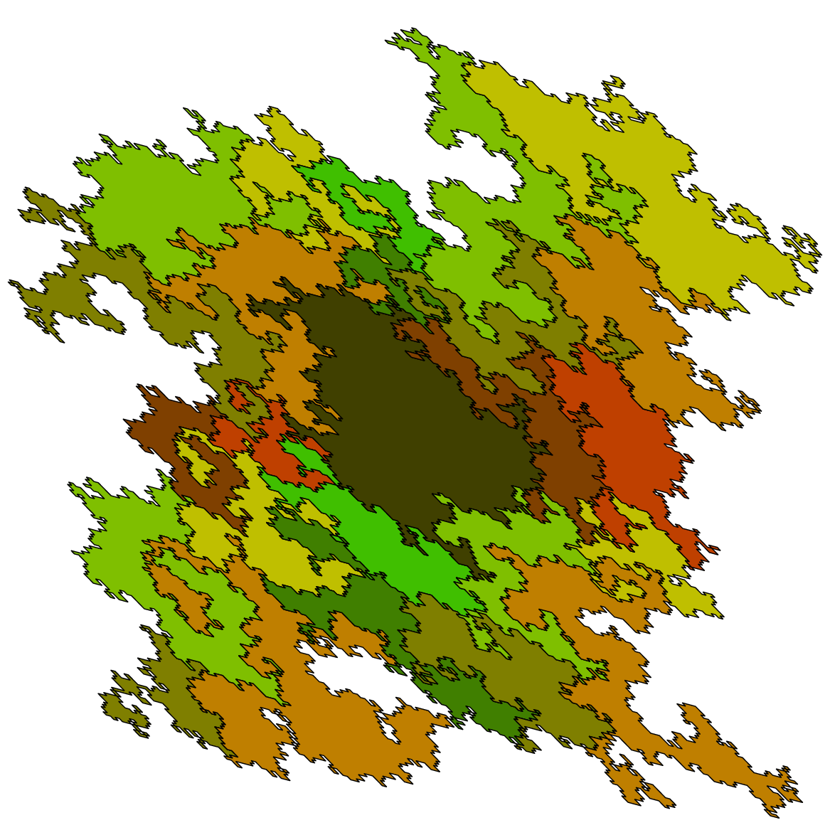
Example 3.13.

For 𝐫=(34,1)\mathbf{r}=(\frac{3}{4},1), the tiles 𝒯𝐫​(𝐱)\mathcal{T}_{\mathbf{r}}(\mathbf{x}) with ‖𝐱‖∞≤2\|\mathbf{x}\|_{\infty}\leq 2 are depicted in Figure 3. As 𝐫∈𝒟d(0)\mathbf{r}\in\mathcal{D}_{d}^{(0)}, we will see in Corollary 4.7 that the collection {𝒯𝐫​(𝐱)∣𝐱∈ℤd}\{\mathcal{T}_{\mathbf{r}}(\mathbf{x})\mid\mathbf{x}\in\mathbb{Z}^{d}\} is a weak tiling of ℝd\mathbb{R}^{d}.

Refer to caption
Figure 3. The SRS tiles 𝒯𝐫​(𝐱)\mathcal{T}_{\mathbf{r}}(\mathbf{x}) with ‖𝐱‖∞≤2\|\mathbf{x}\|_{\infty}\leq 2 corresponding to 𝐫=(34,1)\mathbf{r}=(\frac{3}{4},1).

4. Multiple tilings and tiling conditions

According to Proposition 3.7, the family {𝒯𝐫​(𝐱)∣𝐱∈ℤd}\{\mathcal{T}_{\mathbf{r}}(\mathbf{x})\mid\mathbf{x}\in\mathbb{Z}^{d}\} of SRS tiles forms a covering of ℝd\mathbb{R}^{d}. Various tiling conditions concerning CNS and beta-tiles are spread in the literature (see e.g. the references in [14, 17]). They are of a combinatorial or dynamical nature, or they are expressed in terms of number systems. Among these conditions, the fact that 𝟎\mathbf{0} is an inner point of the central tile plays an important role, which is related to the finiteness property (F) introduced and discussed in Sections 6 (see e.g. [2] for the case of beta-tiles).

In this section, we study tiling properties of SRS tiles. The notions of covering and tiling we will use here are discussed in Section 4.1. In Section 4.2, some facts on mm-exclusive points are shown. A sufficient condition for coverings to be in fact tilings is given in Section 4.3.

4.1. Coverings and tilings

According to Lemma 3.3 and Proposition 3.7, the family of SRS tiles {𝒯𝐫​(𝐱)∣𝐱∈ℤd}\{\mathcal{T}_{\mathbf{r}}(\mathbf{x})\mid\mathbf{x}\in\mathbb{Z}^{d}\} is a covering with bounded degree, that is, every point 𝐭∈ℝd\mathbf{t}\in\mathbb{R}^{d} is contained in a finite and uniformly bounded number of tiles. Thus there exists a unique positive integer mm such that every point 𝐭∈ℝd\mathbf{t}\in\mathbb{R}^{d} is contained in at least mm SRS tiles and there exists a point that is contained in exactly mm tiles. Let us introduce several definitions concerning the notions of covering and tiling.

Definition 4.1 (Covering and tiling; exclusive and inner point).

Let 𝒦\mathcal{K} be a locally finite collection of compact subsets covering ℝd\mathbb{R}^{d}.

  • •

    The covering degree with respect to 𝒦\mathcal{K} of a point 𝐭∈ℝd\mathbf{t}\in\mathbb{R}^{d} is given by deg⁡(𝒦,𝐭):=#⁡{K∈𝒦∣𝐭∈K}\deg(\mathcal{K},\mathbf{t}):=\#\{K\in\mathcal{K}\mid\mathbf{t}\in K\}.

  • •

    The covering degree of 𝒦\mathcal{K} is given by deg⁡(𝒦):=min⁡{deg⁡(𝒦,𝐭)∣𝐭∈ℝd}\deg(\mathcal{K}):=\min\{\deg(\mathcal{K},\mathbf{t})\mid\mathbf{t}\in\mathbb{R}^{d}\}.

  • •

    The collection 𝒦\mathcal{K} is a weak mm-tiling if deg⁡(𝒦)=m\deg(\mathcal{K})=m and ⋂i=1m+1int⁡(Ki)=∅\bigcap_{i=1}^{m+1}\mathrm{int}(K_{i})=\emptyset for every choice of m+1m+1 pairwise different K1,…,Km+1∈𝒦K_{1},\ldots,K_{m+1}\in\mathcal{K}. A weak 11-tiling is also called weak tiling.

  • •

    A point 𝐭∈ℝd\mathbf{t}\in\mathbb{R}^{d} is mm-exclusive with respect to 𝒦\mathcal{K} if deg⁡(𝒦,𝐭)=deg⁡(𝒦)=m\deg(\mathcal{K},\mathbf{t})=\deg(\mathcal{K})=m.

  • •

    A point 𝐭∈ℝd\mathbf{t}\in\mathbb{R}^{d} is an inner point of the collection 𝒦\mathcal{K} if 𝐭∉⋃K∈𝒦∂K\mathbf{t}\not\in\bigcup_{K\in\mathcal{K}}\partial K.

In particular, the collection 𝒦\mathcal{K} is a weak tiling if each inner point of 𝒦\mathcal{K} belongs to exactly one element of 𝒦\mathcal{K}. Moreover, the definition of 11-exclusive points with respect to {𝒯𝐫​(𝐱)∣𝐱∈ℤd}\{\mathcal{T}_{\mathbf{r}}(\mathbf{x})\mid{\mathbf{x}\in\mathbb{Z}^{d}}\} recovers the notion of exclusive points introduced in Section 3.3.

Let us recall that a tiling by translation is often defined as a collection of tiles having finitely many tiles up to translation, with a tile being assumed to be the closure of its interior. We study weak tilings in the sense of Definition 4.1 because of the following reasons:

  • •

    There exist choices of 𝐫∈int⁡(𝒟d)\mathbf{r}\in\mathrm{int}(\mathcal{D}_{d}), 𝐱∈ℤd\mathbf{x}\in\mathbb{Z}^{d}, such that the tile 𝒯𝐫​(𝐱)\mathcal{T}_{\mathbf{r}}(\mathbf{x}) is not the closure of its interior, see Example 3.12.

  • •

    There exist parameters 𝐫∈int⁡(𝒟d)\mathbf{r}\in\mathrm{int}(\mathcal{D}_{d}) such that the family {𝒯𝐫​(𝐱)∣𝐱∈ℤd}\{\mathcal{T}_{\mathbf{r}}(\mathbf{x})\mid{\mathbf{x}\in\mathbb{Z}^{d}}\} is not a collection of finitely many tiles up to translation, e.g. 𝐫=(−2/3)\mathbf{r}=(-2/3), see Corollary 5.20. We conjecture that this holds for every 𝐫\mathbf{r} related to a non-monic CNS (see Section 5) or a non-unit Pisot number (see Section 6).

  • •

    We are not able to show that the boundaries of the tiles 𝒯𝐫​(𝐱)\mathcal{T}_{\mathbf{r}}(\mathbf{x}) have zero dd-dimensional Lebesgue measure. If 𝐫\mathbf{r} is related to a monic CNS or a unit Pisot number, the fact that the boundary of each tile has zero measure is a direct consequence of the self-affine structure of the boundary of the tiles (cf. [3, 25, 30]). For other parameters 𝐫\mathbf{r}, we have no appropriate description of the boundary, and we cannot evaluate its measure.

We are now going to prove that, for a large class of parameters 𝐫\mathbf{r}, the collection {𝒯𝐫​(𝐱)∣𝐱∈ℤd}\{\mathcal{T}_{\mathbf{r}}(\mathbf{x})\mid{\mathbf{x}\in\mathbb{Z}^{d}}\} is a weak mm-tiling, by showing that the set of mm-exclusive points is dense in ℝd\mathbb{R}^{d}.

4.2. mm-exclusive points

Let us first prove that mm-exclusive points are always inner points of {𝒯𝐫​(𝐱)∣𝐱∈ℤd}\{\mathcal{T}_{\mathbf{r}}(\mathbf{x})\mid{\mathbf{x}\in\mathbb{Z}^{d}}\}.

Lemma 4.2.

Let 𝐫∈int⁡(𝒟d)\mathbf{r}\in\mathrm{int}(\mathcal{D}_{d}) be reduced and let mm be the covering degree of {𝒯𝐫​(𝐱)∣𝐱∈ℤd}\{\mathcal{T}_{\mathbf{r}}(\mathbf{x})\mid\mathbf{x}\in\mathbb{Z}^{d}\}. Then there exists an mm-exclusive point. Every mm-exclusive point 𝐭∈⋂i=1m𝒯𝐫​(𝐱i)\mathbf{t}\in\bigcap_{i=1}^{m}\mathcal{T}_{\mathbf{r}}(\mathbf{x}_{i}) satisfies 𝐭∈⋂i=1mint⁡(𝒯𝐫​(𝐱i))\mathbf{t}\in\bigcap_{i=1}^{m}\mathrm{int}(\mathcal{T}_{\mathbf{r}}(\mathbf{x}_{i})). In particular, mm-exclusive points are inner points of {𝒯𝐫​(𝐱)∣𝐱∈ℤd}\{\mathcal{T}_{\mathbf{r}}(\mathbf{x})\mid\mathbf{x}\in\mathbb{Z}^{d}\}.

Proof.

The existence of an mm-exclusive point is a direct consequence of the definition of the covering degree.

Assume that 𝐭\mathbf{t} is an mm-exclusive point. Let 𝒯𝐫​(𝐱1),…,𝒯𝐫​(𝐱m)\mathcal{T}_{\mathbf{r}}(\mathbf{x}_{1}),\ldots,\mathcal{T}_{\mathbf{r}}(\mathbf{x}_{m}) be the mm tiles it belongs to. Assume that there exists a sequence of points (𝐭n)n∈ℕ(\mathbf{t}_{n})_{n\in\mathbb{N}} with values in ℝd\mathbb{R}^{d} such that limn→∞𝐭n=𝐭\lim_{n\to\infty}\mathbf{t}_{n}=\mathbf{t}, and a sequence of points (𝐳n)n∈ℕ(\mathbf{z}_{n})_{n\in\mathbb{N}} with values in ℤd\mathbb{Z}^{d} such that 𝐭n∈𝒯𝐫​(𝐳n)\mathbf{t}_{n}\in\mathcal{T}_{\mathbf{r}}(\mathbf{z}_{n}) for all n∈ℕn\in\mathbb{N}, with 𝐳n\mathbf{z}_{n} distinct from all 𝐱i\mathbf{x}_{i}’s. Since the collection is locally finite, an infinite subsequence of 𝐳n\mathbf{z}_{n}’s is constant, say equal to 𝐳\mathbf{z}. Since the tiles are compact, this implies that 𝐭∈𝒯𝐫​(𝐳)\mathbf{t}\in\mathcal{T}_{\mathbf{r}}(\mathbf{z}), which contradicts the mm-exclusivity. Thus there exists a neighbourhood UU of 𝐭\mathbf{t} with U∩𝒯𝐫​(𝐳)=∅U\cap\mathcal{T}_{\mathbf{r}}(\mathbf{z})=\emptyset for each 𝐳∈ℤd∖{𝐱1,…,𝐱m}\mathbf{z}\in\mathbb{Z}^{d}\setminus\{\mathbf{x}_{1},\ldots,\mathbf{x}_{m}\}. By the mm-covering property, we know that each point belongs to at least mm tiles, which implies that U⊆⋂i=1m𝒯𝐫​(𝐱i)U\subseteq\bigcap_{i=1}^{m}\mathcal{T}_{\mathbf{r}}(\mathbf{x}_{i}). ∎

Let us now prove that an mm-exclusive point 𝐭∈⋂i=1m𝒯𝐫​(𝐱i)\mathbf{t}\in\bigcap_{i=1}^{m}\mathcal{T}_{\mathbf{r}}(\mathbf{x}_{i}) is somehow characterized by any sequence of approximations M𝐫n​𝐳−nM_{\mathbf{r}}^{n}\mathbf{z}_{-n} defined in Proposition 3.6. Note that 𝐭=Limn→∞M𝐫n​𝒯𝐫​(𝐳−n)\mathbf{t}=\mathop{\rm Lim}_{n\to\infty}M_{\mathbf{r}}^{n}\mathcal{T}_{\mathbf{r}}(\mathbf{z}_{-n}), and that M𝐫n​𝒯𝐫​(𝐳−n)M_{\mathbf{r}}^{n}\mathcal{T}_{\mathbf{r}}(\mathbf{z}_{-n}) is a tile in the nn-fold subdivision 𝒯𝐫​(𝐱i)=⋃𝐳∈τ𝐫−n​(𝐱i)M𝐫n​𝒯𝐫​(𝐳)\mathcal{T}_{\mathbf{r}}(\mathbf{x}_{i})=\bigcup_{\mathbf{z}\in\tau_{\mathbf{r}}^{-n}(\mathbf{x}_{i})}M_{\mathbf{r}}^{n}\mathcal{T}_{\mathbf{r}}(\mathbf{z}) for some 𝐱i\mathbf{x}_{i}, which is given by applying (3.3) nn times. The following proposition states that a point 𝐭\mathbf{t} is mm-exclusive provided that, for some n∈ℕn\in\mathbb{N}, each M𝐫n​𝒯𝐫​(𝐳−n+𝐲)M_{\mathbf{r}}^{n}\mathcal{T}_{\mathbf{r}}(\mathbf{z}_{-n}+\mathbf{y}) with ‖𝐲‖≤2​R\|\mathbf{y}\|\leq 2R occurs in the subdivision of some tile 𝒯𝐫​(𝐱i)\mathcal{T}_{\mathbf{r}}(\mathbf{x}_{i}), 1≤i≤m1\leq i\leq m.

Proposition 4.3.

Let mm be the covering degree of {𝒯𝐫​(𝐱)∣𝐱∈ℤd}\{\mathcal{T}_{\mathbf{r}}(\mathbf{x})\mid\mathbf{x}\in\mathbb{Z}^{d}\}, 𝐭∈ℝd\mathbf{t}\in\mathbb{R}^{d}, (𝐳−n)n∈ℕ(\mathbf{z}_{-n})_{n\in\mathbb{N}} as in Proposition 3.6, and RR defined by (3.1). Then 𝐭\mathbf{t} is mm-exclusive and contained in the intersection ⋂i=1m𝒯𝐫​(𝐱i)\bigcap_{i=1}^{m}\mathcal{T}_{\mathbf{r}}(\mathbf{x}_{i}) if and only if there exists some n∈ℕn\in\mathbb{N} such that

(4.1) τ𝐫n​(𝐳−n+𝐲)∈{𝐱1,…,𝐱m}for all​𝐲∈ℤd​with​‖𝐲‖≤2​R.\tau_{\mathbf{r}}^{n}(\mathbf{z}_{-n}+\mathbf{y})\in\{\mathbf{x}_{1},\ldots,\mathbf{x}_{m}\}\quad\mbox{for all}\ \mathbf{y}\in\mathbb{Z}^{d}\ \mbox{with}\ \|\mathbf{y}\|\leq 2R.

If, for some 𝐳∈ℤd\mathbf{z}\in\mathbb{Z}^{d}, n∈ℕn\in\mathbb{N},

(4.2) #{τ𝐫n(𝐳+𝐲)∣𝐲∈ℤd,∥𝐲∥≤R}=m,\#\{\tau_{\mathbf{r}}^{n}(\mathbf{z}+\mathbf{y})\mid\mathbf{y}\in\mathbb{Z}^{d},\,\|\mathbf{y}\|\leq R\big\}=m,

then M𝐫n​𝐳M_{\mathbf{r}}^{n}\mathbf{z} is an mm-exclusive point.

Proof.

Assume that 𝐭\mathbf{t} is an mm-exclusive point. By Lemma 4.2, there exists some ε>0\varepsilon>0 such that every point 𝐭′∈ℝd\mathbf{t}^{\prime}\in\mathbb{R}^{d} satisfying ‖𝐭′−𝐭‖<ε\|\mathbf{t}^{\prime}-\mathbf{t}\|<\varepsilon lies only in the tiles 𝒯𝐫​(𝐱1),…,𝒯𝐫​(𝐱m)\mathcal{T}_{\mathbf{r}}(\mathbf{x}_{1}),\,\ldots,\,\mathcal{T}_{\mathbf{r}}(\mathbf{x}_{m}). Let n∈ℕn\in\mathbb{N} satisfy 4​ρ~n​R<ε4\tilde{\rho}^{n}R<\varepsilon. Since M𝐫−n​𝐭∈𝒯𝐫​(𝐳−n)M_{\mathbf{r}}^{-n}\mathbf{t}\in\mathcal{T}_{\mathbf{r}}(\mathbf{z}_{-n}), we have ‖M𝐫−n​𝐭−𝐳−n‖≤R\|M_{\mathbf{r}}^{-n}\mathbf{t}-\mathbf{z}_{-n}\|\leq R by Lemma 3.3, thus ‖𝐭−M𝐫n​(𝐳−n+𝐲)‖≤3​ρ~n​R\|\mathbf{t}-M_{\mathbf{r}}^{n}(\mathbf{z}_{-n}+\mathbf{y})\|\leq 3\tilde{\rho}^{n}R if ‖𝐲‖≤2​R\|\mathbf{y}\|\leq 2R. By Theorem 3.5, there exists a point 𝐭′∈𝒯𝐫​(τ𝐫n​(𝐳−n+𝐲))\mathbf{t}^{\prime}\in\mathcal{T}_{\mathbf{r}}\big(\tau_{\mathbf{r}}^{n}(\mathbf{z}_{-n}+\mathbf{y})\big) with ‖𝐭′−M𝐫n​(𝐳−n+𝐲)‖≤ρ~n​R\|\mathbf{t}^{\prime}-M_{\mathbf{r}}^{n}(\mathbf{z}_{-n}+\mathbf{y})\|\leq\tilde{\rho}^{n}R. Since ‖𝐭′−𝐭‖≤4​ρ~n​R<ε\|\mathbf{t}^{\prime}-\mathbf{t}\|\leq 4\tilde{\rho}^{n}R<\varepsilon, we obtain τ𝐫n​(𝐳−n+𝐲)∈{𝐱1,…,𝐱m}\tau_{\mathbf{r}}^{n}(\mathbf{z}_{-n}+\mathbf{y})\in\{\mathbf{x}_{1},\ldots,\mathbf{x}_{m}\}.

For the other direction, assume that there exists some n∈ℕn\in\mathbb{N} such that (4.1) holds. We have to show that 𝐭∈𝒯𝐫​(𝐳0′)\mathbf{t}\in\mathcal{T}_{\mathbf{r}}(\mathbf{z}_{0}^{\prime}) implies 𝐳0′∈{𝐱1,…,𝐱m}\mathbf{z}_{0}^{\prime}\in\{\mathbf{x}_{1},\ldots,\mathbf{x}_{m}\}. Let (𝐳−n′)n∈ℕ(\mathbf{z}_{-n}^{\prime})_{n\in\mathbb{N}} be as in Proposition 3.6. Since ‖M𝐫−n​𝐭−𝐳−n′‖≤R\|M_{\mathbf{r}}^{-n}\mathbf{t}-\mathbf{z}_{-n}^{\prime}\|\leq R and ‖M𝐫−n​𝐭−𝐳−n‖≤R\|M_{\mathbf{r}}^{-n}\mathbf{t}-\mathbf{z}_{-n}\|\leq R, (4.1) implies τ𝐫n​(𝐳−n′)∈{𝐱1,…,𝐱m}\tau_{\mathbf{r}}^{n}(\mathbf{z}_{-n}^{\prime})\in\{\mathbf{x}_{1},\ldots,\mathbf{x}_{m}\}. Since 𝐳0′=τ𝐫n​(𝐳−n′)\mathbf{z}_{0}^{\prime}=\tau_{\mathbf{r}}^{n}(\mathbf{z}_{-n}^{\prime}), the point 𝐭\mathbf{t} is mm-exclusive.

For the second statement, let {τ𝐫n(𝐳+𝐲)∣𝐲∈ℤd,∥𝐲∥≤R}={𝐱1,…,𝐱m}\{\tau_{\mathbf{r}}^{n}(\mathbf{z}+\mathbf{y})\mid\mathbf{y}\in\mathbb{Z}^{d},\,\|\mathbf{y}\|\leq R\big\}=\{\mathbf{x}_{1},\ldots,\mathbf{x}_{m}\}, M𝐫n​𝐳∈𝒯𝐫​(𝐳0′)M_{\mathbf{r}}^{n}\mathbf{z}\in\mathcal{T}_{\mathbf{r}}(\mathbf{z}_{0}^{\prime}), and (𝐳−n′)n∈ℕ(\mathbf{z}_{-n}^{\prime})_{n\in\mathbb{N}} be as in Proposition 3.6, with 𝐭=M𝐫n​𝐳\mathbf{t}=M_{\mathbf{r}}^{n}\mathbf{z}. Then we have ‖𝐳−n′−𝐳‖≤R\|\mathbf{z}_{-n}^{\prime}-\mathbf{z}\|\leq R, thus 𝐳0′∈{𝐱1,…,𝐱m}\mathbf{z}_{0}^{\prime}\in\{\mathbf{x}_{1},\ldots,\mathbf{x}_{m}\} and M𝐫n​𝐳M_{\mathbf{r}}^{n}\mathbf{z} is mm-exclusive. ∎

Note that Proposition 4.3 provides an easy way to show that a point is mm-exclusive. However, it does not provide a finite method to prove that a point is not mm-exclusive.

The following corollary of Proposition 4.3 permits us to obtain an mm-exclusive point from another one, by finding a translation preserving the local configuration of tiles up to the nn-th level, with nn such that (4.2) holds.

Corollary 4.4.

Let mm be the covering degree of {𝒯𝐫​(𝐱)∣𝐱∈ℤd}\{\mathcal{T}_{\mathbf{r}}(\mathbf{x})\mid\mathbf{x}\in\mathbb{Z}^{d}\}, and assume that 𝐳∈ℤd\mathbf{z}\in\mathbb{Z}^{d}, n∈ℕn\in\mathbb{N} satisfy (4.2). Let 𝐚∈ℤd\mathbf{a}\in\mathbb{Z}^{d}. If there exists some 𝐛∈ℤd\mathbf{b}\in\mathbb{Z}^{d} such that

τ𝐫n​(𝐳+𝐚+𝐲)=τ𝐫n​(𝐳+𝐲)+𝐛for all ​𝐲∈ℤd​ with ​‖𝐲‖≤R,\tau_{\mathbf{r}}^{n}(\mathbf{z}+\mathbf{a}+\mathbf{y})=\tau_{\mathbf{r}}^{n}(\mathbf{z}+\mathbf{y})+\mathbf{b}\quad\mbox{for all }\mathbf{y}\in\mathbb{Z}^{d}\mbox{ with }\|\mathbf{y}\|\leq R,

then M𝐫n​(𝐳+𝐚)M_{\mathbf{r}}^{n}(\mathbf{z}+\mathbf{a}) is an mm-exclusive point.

A simple way to obtain an infinite number of mm-exclusive points from one mm-exclusive point 𝐭≠𝟎\mathbf{t}\neq\mathbf{0} is provided by the following lemma.

Lemma 4.5.

If 𝐭\mathbf{t} is an mm-exclusive point, then M𝐫​𝐭M_{\mathbf{r}}\mathbf{t} is an mm-exclusive point.

Proof.

If M𝐫​𝐭∈𝒯𝐫​(𝐱i)M_{\mathbf{r}}\mathbf{t}\in\mathcal{T}_{\mathbf{r}}(\mathbf{x}_{i}), then there exists some 𝐲i∈τ𝐫−1​(𝐱i)\mathbf{y}_{i}\in\tau_{\mathbf{r}}^{-1}(\mathbf{x}_{i}) such that 𝐭∈𝒯𝐫​(𝐲i)\mathbf{t}\in\mathcal{T}_{\mathbf{r}}(\mathbf{y}_{i}), and all 𝐲i\mathbf{y}_{i} are mutually different if the 𝐱i\mathbf{x}_{i} are. Therefore the number of tiles to which a point M𝐫​𝐭M_{\mathbf{r}}\mathbf{t} belongs cannot be larger than that for 𝐭\mathbf{t}. ∎

4.3. Weak mm-tilings

In what follows we will establish our tiling results. In order to prove these results we first show that if 𝐫\mathbf{r} has certain algebraic properties then there exists a set that is relatively dense in ℝd\mathbb{R}^{d} containing only vectors that stabilize the configuration of tiles. Together with Corollary 4.4 and Lemma 4.5, this will prove that {𝒯𝐫​(𝐱)∣𝐱∈ℤd}\{\mathcal{T}_{\mathbf{r}}(\mathbf{x})\mid\mathbf{x}\in\mathbb{Z}^{d}\} forms a weak mm-tiling. If 𝐫\mathbf{r} also satisfies the finiteness property, it even forms a weak tiling.

Theorem 4.6.

Let 𝐫=(r0,…,rd−1)∈int⁡(𝒟d)\mathbf{r}=(r_{0},\ldots,r_{d-1})\in\mathrm{int}(\mathcal{D}_{d}) with r0≠0r_{0}\neq 0, let mm be the covering degree of {𝒯𝐫​(𝐱)∣𝐱∈ℤd}\{\mathcal{T}_{\mathbf{r}}(\mathbf{x})\mid\mathbf{x}\in\mathbb{Z}^{d}\}, and assume that 𝐫\mathbf{r} satisfies one of the following conditions:

  • •

    𝐫∈ℚd\mathbf{r}\in\mathbb{Q}^{d},

  • •

    (x−β)​(xd+rd−1​xd−1+⋯+r1​x+r0)∈ℤ⁡[x](x-\beta)(x^{d}+r_{d-1}x^{d-1}+\cdots+r_{1}x+r_{0})\in\mathbb{Z}[x] for some β>1\beta>1,

  • •

    r0,…,rd−1r_{0},\ldots,r_{d-1} are algebraically independent over ℚ\mathbb{Q}.

Then the set of mm-exclusive points is dense in ℝd\mathbb{R}^{d}, and {𝒯𝐫​(𝐱)∣𝐱∈ℤd}\{\mathcal{T}_{\mathbf{r}}(\mathbf{x})\mid\mathbf{x}\in\mathbb{Z}^{d}\} is a weak mm-tiling.

Proof.

By the definition of the covering degree (Definition 4.1), there exists an mm-exclusive point 𝐭\mathbf{t} with respect to {𝒯𝐫​(𝐱)∣𝐱∈ℤd}\{\mathcal{T}_{\mathbf{r}}(\mathbf{x})\mid\mathbf{x}\in\mathbb{Z}^{d}\}. Thus the first part of Proposition 4.3 implies that there exist 𝐳∈ℤd\mathbf{z}\in\mathbb{Z}^{d} and n∈ℕn\in\mathbb{N} satisfying (4.2). If we find a relatively dense set Λ\Lambda of vectors 𝐚∈ℤd\mathbf{a}\in\mathbb{Z}^{d} satisfying the conditions of Corollary 4.4, then the set {M𝐫n​(𝐳+𝐚)∣𝐚∈Λ}\{M_{\mathbf{r}}^{n}(\mathbf{z}+\mathbf{a})\mid\mathbf{a}\in\Lambda\} forms a set of mm-exclusive inner points which is relatively dense in ℝd\mathbb{R}^{d}. Applying Lemma 4.5 to the elements of this set yields that the set of mm-exclusive points is dense in ℝd\mathbb{R}^{d}. In view of Definition 4.1, this already proves that {𝒯𝐫​(𝐱)∣𝐱∈ℤd}\{\mathcal{T}_{\mathbf{r}}(\mathbf{x})\mid\mathbf{x}\in\mathbb{Z}^{d}\} forms a weak mm-tiling.

It remains to find a relatively dense set Λ\Lambda of vectors 𝐚∈ℤd\mathbf{a}\in\mathbb{Z}^{d} satisfying the conditions of Corollary 4.4. This is done separately for each of the three classes of parameters given in the statement of the theorem.

Case 1: 𝐫∈ℚd\mathbf{r}\in\mathbb{Q}^{d}. Let 𝐳∈ℤd\mathbf{z}\in\mathbb{Z}^{d} and n∈ℕn\in\mathbb{N} satisfying (4.2) be given as above. Choose q∈ℕq\in\mathbb{N} in a way that 𝐫∈q−1​ℤd\mathbf{r}\in q^{-1}{\mathbb{Z}}^{d}. Then we have for every 𝐱,𝐚∈ℤd\mathbf{x},\mathbf{a}\in\mathbb{Z}^{d}, k≥1k\geq 1,

τ𝐫​(𝐱+qk​𝐚)=M𝐫​(𝐱+qk​𝐚)+(0,…,0,{𝐫⁡(𝐱+qk​𝐚)})=τ𝐫​(𝐱)+qk−1​𝐚′\tau_{\mathbf{r}}(\mathbf{x}+q^{k}\mathbf{a})=M_{\mathbf{r}}(\mathbf{x}+q^{k}\mathbf{a})+\big(0,\ldots,0,\big\{\mathbf{r}(\mathbf{x}+q^{k}\mathbf{a})\big\}\big)=\tau_{\mathbf{r}}(\mathbf{x})+q^{k-1}\mathbf{a}^{\prime}

for some 𝐚′∈ℤd\mathbf{a}^{\prime}\in\mathbb{Z}^{d} which does not depend on 𝐱\mathbf{x}. Iterating this, we get that τ𝐫n​(𝐱+qn​𝐚)=τ𝐫n​(𝐱)+𝐛\tau_{\mathbf{r}}^{n}(\mathbf{x}+q^{n}\mathbf{a})=\tau_{\mathbf{r}}^{n}(\mathbf{x})+\mathbf{b} for some 𝐛∈ℤd\mathbf{b}\in\mathbb{Z}^{d} which does not depend on 𝐱\mathbf{x}. In particular, this implies that

τ𝐫n(𝐱+qn𝐚+𝐲)=τ𝐫n(𝐱+𝐲)+𝐛for all 𝐲∈ℤd with ‖𝐲‖≤R.\tau_{\mathbf{r}}^{n}(\mathbf{x}+q^{n}\mathbf{a}+\mathbf{y})=\tau_{\mathbf{r}}^{n}(\mathbf{x}+\mathbf{y})+\mathbf{b}\quad\hbox{for all $\mathbf{y}\in\mathbb{Z}^{d}$ with $\|\mathbf{y}\|\leq R$}.

Thus each element of the set Λ:={qn​𝐚∣𝐚∈ℤd}\Lambda:=\{q^{n}\mathbf{a}\mid\mathbf{a}\in\mathbb{Z}^{d}\} satisfies the conditions of Corollary 4.4. As Λ\Lambda is relatively dense in ℝd\mathbb{R}^{d}, we are done in this case.

Case 2: A⁡(x)=(x−β)​(xd+rd−1​xd−1+⋯+r1​x+r0)∈ℤ⁡[x]A(x)=(x-\beta)(x^{d}+r_{d-1}x^{d-1}+\cdots+r_{1}x+r_{0})\in\mathbb{Z}[x] for some β>1\beta>1. Let 𝐳∈ℤd\mathbf{z}\in\mathbb{Z}^{d} and n∈ℕn\in\mathbb{N} satisfying (4.2) be given as above. Since 𝐫∈int⁡(𝒟d)\mathbf{r}\in\mathrm{int}(\mathcal{D}_{d}), all roots of xd+rd−1​xd−1+⋯+r1​x+r0x^{d}+r_{d-1}x^{d-1}+\cdots+r_{1}x+r_{0} have modulus less than 11. Therefore, A⁡(x)A(x) is irreducible. (Indeed, β\beta is a Pisot number.) Let

ε:=min‖𝐲‖≤R, 0≤k<n⁡β−k​(1−{𝐫​τ𝐫k​(𝐳+𝐲)})>0.\varepsilon:=\min_{\|\mathbf{y}\|\leq R,\,0\leq k<n}\beta^{-k}\big(1-\big\{\mathbf{r}\tau_{\mathbf{r}}^{k}(\mathbf{z}+\mathbf{y})\big\}\big)>0.

From the definition of τ𝐫\tau_{\mathbf{r}} we know that for every 𝐱\mathbf{x}, 𝐚∈ℤd\mathbf{a}\in\mathbb{Z}^{d}, one has τ𝐫​(𝐱+𝐚)=τ𝐫​(𝐱)+τ𝐫​(𝐚)\tau_{\mathbf{r}}(\mathbf{x}+\mathbf{a})=\tau_{\mathbf{r}}(\mathbf{x})+\tau_{\mathbf{r}}(\mathbf{a}) if and only if {𝐫𝐱+𝐫𝐚}={𝐫𝐱}+{𝐫𝐚}\{\mathbf{r}\mathbf{x}+\mathbf{r}\mathbf{a}\}=\{\mathbf{r}\mathbf{x}\}+\{\mathbf{r}\mathbf{a}\}. In Proposition 6.1, we will see that {𝐫​τ𝐫k​(𝐚)}=Tβk​({𝐫𝐚})\{\mathbf{r}\tau_{\mathbf{r}}^{k}(\mathbf{a})\}=T_{\beta}^{k}(\{\mathbf{r}\mathbf{a}\}), where TβT_{\beta} is the β\beta-transformation defined in Section 6.1. If we choose 𝐚∈ℤd\mathbf{a}\in\mathbb{Z}^{d} such that {𝐫𝐚}<ε\{\mathbf{r}\mathbf{a}\}<\varepsilon, then we get {𝐫​τ𝐫k​(𝐚)}=βk​{𝐫𝐚}\{\mathbf{r}\tau_{\mathbf{r}}^{k}(\mathbf{a})\}=\beta^{k}\{\mathbf{r}\mathbf{a}\} for 0≤k<n0\leq k<n, and

(4.3) τ𝐫k​(𝐳+𝐚+𝐲)=τ𝐫k​(𝐳+𝐲)+τ𝐫k​(𝐚)for all ​‖𝐲‖≤R, 0≤k≤n.\tau_{\mathbf{r}}^{k}(\mathbf{z}+\mathbf{a}+\mathbf{y})=\tau_{\mathbf{r}}^{k}(\mathbf{z}+\mathbf{y})+\tau_{\mathbf{r}}^{k}(\mathbf{a})\quad\mbox{for all }\|\mathbf{y}\|\leq R,\,0\leq k\leq n.

Thus each element of the set Λ:={𝐚∈ℤd∣{𝐫𝐚}<ε}\Lambda:=\{\mathbf{a}\in\mathbb{Z}^{d}\mid\{\mathbf{r}\mathbf{a}\}<\varepsilon\} satisfies the conditions of Corollary 4.4. Since A⁡(x)A(x) is irreducible, the coordinates of 𝐫\mathbf{r} are linearly independent over ℚ\mathbb{Q}. Thus Kronecker’s theorem yields that Λ\Lambda is relatively dense in ℝd\mathbb{R}^{d} and we are done also in this case.

Case 3: r0,…,rd−1r_{0},\ldots,r_{d-1} are algebraically independent. Let 𝐳∈ℤd\mathbf{z}\in\mathbb{Z}^{d} and n∈ℕn\in\mathbb{N} satisfying (4.2) be given as above. Set

εk:=min‖𝐲‖≤R⁡(1−{𝐫​τ𝐫k​(𝐳+𝐲)})for ​0≤k<n.\varepsilon_{k}:=\min_{\|\mathbf{y}\|\leq R}\big(1-\big\{\mathbf{r}\tau_{\mathbf{r}}^{k}(\mathbf{z}+\mathbf{y})\big\}\big)\quad\mbox{for }0\leq k<n.

We have εk>0\varepsilon_{k}>0. Similarly to Case 2, each element of the set

Λ:={𝐚∈ℤd∣{𝐫τ𝐫k(𝐚)}<εk for 0≤k<n}\Lambda:=\{\mathbf{a}\in\mathbb{Z}^{d}\mid\{\mathbf{r}\tau_{\mathbf{r}}^{k}(\mathbf{a})\}<\varepsilon_{k}\hbox{ for }0\leq k<n\}

satisfies (4.3). Thus each 𝐚∈Λ\mathbf{a}\in\Lambda satisfies the conditions of Corollary 4.4. It remains to prove that Λ\Lambda is relatively dense in ℝd\mathbb{R}^{d}. To this matter we need the following notations. Let ⌊x⌉\lfloor x\rceil denote the nearest integer to x∈ℝx\in\mathbb{R} (with ⌊z+1/2⌉=z\lfloor z+1/2\rceil=z for z∈ℤz\in\mathbb{Z}), let {x}c=x−⌊x⌉\{x\}_{c}=x-\lfloor x\rceil be the “centralized fractional part” and set

τ~𝐫​(𝐱)=M𝐫​𝐱+(0,…,0,{𝐫𝐱}c).\widetilde{\tau}_{\mathbf{r}}(\mathbf{x})=M_{\mathbf{r}}\mathbf{x}+(0,\ldots,0,\{\mathbf{r}\mathbf{x}\}_{c}).

Consider the partition Λ=⋃η∈{0,1}nΛη\Lambda=\bigcup_{\eta\in\{0,1\}^{n}}\Lambda_{\eta} with

Λη:={𝐚∈ℤd∣{𝐫​τ𝐫k​(𝐚)}∈ηk​εk/2+[0,εk/2)​ for ​0≤k<n}(η∈{0,1}n)\Lambda_{\eta}:=\{\mathbf{a}\in\mathbb{Z}^{d}\mid\{\mathbf{r}\tau_{\mathbf{r}}^{k}(\mathbf{a})\}\in\eta_{k}\varepsilon_{k}/2+[0,\varepsilon_{k}/2)\hbox{ for }0\leq k<n\}\qquad(\eta\in\{0,1\}^{n})

(here η=(η0,…,ηn−1)\eta=(\eta_{0},\ldots,\eta_{n-1})). We will prove the following claim.

Claim. Let 𝐞j\mathbf{e}_{j}, 1≤j≤d1\leq j\leq d, be the canonical unit vectors. For each η∈{0,1}n\eta\in\{0,1\}^{n} and j∈{1,…,d}j\in\{1,\ldots,d\}, there exists zη,j∈ℤz_{\eta,j}\in\mathbb{Z} with

(4.4) {𝐫τ~𝐫k(zη,j𝐞j)}c∈(−1)ηk[0,εk/2)for all 0≤k<n.\big\{\mathbf{r}\widetilde{\tau}_{\mathbf{r}}^{k}(z_{\eta,j}\mathbf{e}_{j})\}_{c}\in(-1)^{\eta_{k}}[0,\varepsilon_{k}/2)\quad\mbox{for all}\ 0\leq k<n.

Before we prove this claim we show that it implies the relative denseness of Λ\Lambda in ℝd\mathbb{R}^{d}. Indeed, let η∈{0,1}n\eta\in\{0,1\}^{n} and j∈{1,…,d}j\in\{1,\ldots,d\} be arbitrary. Then the claim yields that for each 𝐚∈Λη\mathbf{a}\in\Lambda_{\eta} we have

{𝐫​τ𝐫k​(𝐚+zη,j​𝐞j)}={𝐫⁡(τ𝐫k​(𝐚)+τ~𝐫k​(zη,j​𝐞j))}={𝐫​τ𝐫k​(𝐚)}+{𝐫​τ~𝐫k​(zη,j​𝐞j)}c∈[0,εk)\big\{\mathbf{r}\tau_{\mathbf{r}}^{k}(\mathbf{a}+z_{\eta,j}\mathbf{e}_{j})\big\}=\big\{\mathbf{r}\big(\tau_{\mathbf{r}}^{k}(\mathbf{a})+\widetilde{\tau}_{\mathbf{r}}^{k}(z_{\eta,j}\mathbf{e}_{j})\big)\big\}=\big\{\mathbf{r}\tau_{\mathbf{r}}^{k}(\mathbf{a})\}+\{\mathbf{r}\widetilde{\tau}_{\mathbf{r}}^{k}(z_{\eta,j}\mathbf{e}_{j})\big\}_{c}\in[0,\varepsilon_{k})

and thus 𝐚+zη,j​𝐞j∈Λ\mathbf{a}+z_{\eta,j}\mathbf{e}_{j}\in\Lambda. Moreover, by analogous reasoning we see that the claim implies the following “dual” result: for each η∈{0,1}n\eta\in\{0,1\}^{n} set η′:=(1,…,1)−η∈{0,1}n\eta^{\prime}:=(1,\ldots,1)-\eta\in\{0,1\}^{n}. Then for each j∈{1,…,d}j\in\{1,\ldots,d\} and each 𝐚∈Λη\mathbf{a}\in\Lambda_{\eta} we have 𝐚−zη′,j​𝐞j∈Λ\mathbf{a}-z_{\eta^{\prime},j}\mathbf{e}_{j}\in\Lambda.

Summing up, the claim implies that from each 𝐚∈Λ\mathbf{a}\in\Lambda there exist other elements of Λ\Lambda in uniformly bounded distance in all positive and negative coordinate directions. This proves that Λ\Lambda is relatively dense in ℝd\mathbb{R}^{d}. Thus it remains to prove the above claim.

To prove this claim let η=(η0,…,ηn−1)∈{0,1}n\eta=(\eta_{0},\ldots,\eta_{n-1})\in\{0,1\}^{n} and j∈{1,…,d}j\in\{1,\ldots,d\} be arbitrary but fixed. We need to find an integer zη,jz_{\eta,j} satisfying (4.4). First observe that for 𝐛∈ℤd\mathbf{b}\in\mathbb{Z}^{d}

(4.5) τ~𝐫k​(𝐛)=M𝐫k​𝐛+∑j=0k−1M𝐫k−j−1​(0,…,0,{𝐫​τ~𝐫j​(𝐛)}c)t.\widetilde{\tau}_{\mathbf{r}}^{k}(\mathbf{b})=M_{\mathbf{r}}^{k}\mathbf{b}+\sum_{j=0}^{k-1}M_{\mathbf{r}}^{k-j-1}\big(0,\ldots,0,\{\mathbf{r}\widetilde{\tau}_{\mathbf{r}}^{j}(\mathbf{b})\}_{c}\big)^{t}.

Let γk={𝐫​M𝐫k​𝐞d}c\gamma_{k}=\{\mathbf{r}M_{\mathbf{r}}^{k}\mathbf{e}_{d}\}_{c}, 0≤k<n0\leq k<n. If the arguments of all centralized fractional parts are small, then multiplying (4.5) by 𝐫\mathbf{r} and applying {⋅}c\{\cdot\}_{c} yields

(4.6) {𝐫​τ~𝐫k​(𝐛)}c={𝐫​M𝐫k​𝐛}c+∑j=0k−1{𝐫​τ~𝐫j​(𝐛)}c​γk−j−1.\{\mathbf{r}\widetilde{\tau}_{\mathbf{r}}^{k}(\mathbf{b})\}_{c}=\{\mathbf{r}M_{\mathbf{r}}^{k}\mathbf{b}\}_{c}+\sum_{j=0}^{k-1}\{\mathbf{r}\widetilde{\tau}_{\mathbf{r}}^{j}(\mathbf{b})\}_{c}\,\gamma_{k-j-1}.

Inserting (4.6) iteratively in itself we gain

{𝐫​τ~𝐫k​(𝐛)}c\displaystyle\{\mathbf{r}\widetilde{\tau}_{\mathbf{r}}^{k}(\mathbf{b})\}_{c} ={𝐫​M𝐫k​𝐛}c+∑k=j0>j1>⋯>jℓ≥0,ℓ≥1{𝐫​M𝐫jℓ​𝐛}c​∏i=0ℓ−1γji−ji+1−1\displaystyle=\{\mathbf{r}M_{\mathbf{r}}^{k}\mathbf{b}\}_{c}+\sum_{k=j_{0}>j_{1}>\cdots>j_{\ell}\geq 0,\,\ell\geq 1}\{\mathbf{r}M_{\mathbf{r}}^{j_{\ell}}\mathbf{b}\}_{c}\prod_{i=0}^{\ell-1}\gamma_{j_{i}-j_{i+1}-1}
=∑h=0k{𝐫​M𝐫h​𝐛}c​∑k=j0>⋯>jℓ=h,ℓ≥0∏i=0ℓ−1γji−ji+1−1.\displaystyle=\sum_{h=0}^{k}\{\mathbf{r}M_{\mathbf{r}}^{h}\mathbf{b}\}_{c}\sum_{k=j_{0}>\cdots>j_{\ell}=h,\,\ell\geq 0}\prod_{i=0}^{\ell-1}\gamma_{j_{i}-j_{i+1}-1}.

Setting

ck:=∑k=j0>⋯>jℓ=0,ℓ≥0∏i=0ℓ−1γji−ji+1−1c_{k}:=\sum_{k=j_{0}>\cdots>j_{\ell}=0,\,\ell\geq 0}\prod_{i=0}^{\ell-1}\gamma_{j_{i}-j_{i+1}-1}

we get

{𝐫​τ~𝐫k​(𝐛)}c=∑h=0kck−h​{𝐫​M𝐫h​𝐛}c.\{\mathbf{r}\widetilde{\tau}_{\mathbf{r}}^{k}(\mathbf{b})\}_{c}=\sum_{h=0}^{k}c_{k-h}\,\{\mathbf{r}M_{\mathbf{r}}^{h}\mathbf{b}\}_{c}.

Now we inductively choose intervals IkI_{k}, 0≤k<n0\leq k<n, satisfying

Ik+∑h=0k−1ck−hIh⊆(−1)ηk[0,εk/2).I_{k}+\sum_{h=0}^{k-1}c_{k-h}I_{h}\subseteq(-1)^{\eta_{k}}[0,\varepsilon_{k}/2).

W.l.o.g., we can choose the intervals IkI_{k} sufficiently small such that (4.6) holds provided that {𝐫​M𝐫k​𝐛}c∈Ik\{\mathbf{r}M_{\mathbf{r}}^{k}\mathbf{b}\}_{c}\in I_{k} for 0≤k<n0\leq k<n.

Since r0,…,rd−1r_{0},\ldots,r_{d-1} are algebraically independent, the numbers {𝐫​M𝐫k​𝐞j}c\{\mathbf{r}M_{\mathbf{r}}^{k}\mathbf{e}_{j}\}_{c}, for 0≤k<n0\leq k<n, are linearly independent over ℚ\mathbb{Q}. Thus Kronecker’s theorem yields the existence of an integer zη,jz_{\eta,j} satisfying {zη,j​𝐫​M𝐫k​𝐞j}c∈Ik\{z_{\eta,j}\mathbf{r}M_{\mathbf{r}}^{k}\mathbf{e}_{j}\}_{c}\in I_{k} for 0≤k<n0\leq k<n, hence, zη,jz_{\eta,j} satisfies (4.4) and we are done. ∎

Since Corollary 3.11 implies that for each SRS with finiteness property the origin is an exclusive point of 𝒯𝐫​(𝟎)\mathcal{T}_{\mathbf{r}}(\mathbf{0}) we gain the following tiling property.

Corollary 4.7.

If 𝐫∈𝒟d(0)\mathbf{r}\in\mathcal{D}_{d}^{(0)} is reduced and satisfies one of the conditions of Theorem 4.6, then {𝒯𝐫​(𝐱)∣𝐱∈ℤd}\{\mathcal{T}_{\mathbf{r}}(\mathbf{x})\mid\mathbf{x}\in\mathbb{Z}^{d}\} is a weak tiling.

Let us stress the fact that we have no general algorithmic criterion to check Proposition 4.3. This is mainly due to the fact that we have no IFS describing the boundary of an SRS tile. Nonetheless, Theorem 4.6 implies a tiling criterion.

Corollary 4.8.

If 𝐫∈int⁡(𝒟d)\mathbf{r}\in\mathrm{int}(\mathcal{D}_{d}) is reduced and satisfies one of the conditions of Theorem 4.6, then the collection {𝒯𝐫​(𝐱)∣𝐱∈ℤd}\{\mathcal{T}_{\mathbf{r}}(\mathbf{x})\mid\mathbf{x}\in\mathbb{Z}^{d}\} is a weak tiling if and only if it has at least one exclusive point.

We conclude this section with a result that treats the case d=1d=1 in a very complete way. (We identify one dimensional vectors with scalars here.)

Theorem 4.9.

Let r∈int⁡(𝒟1)r\in\mathrm{int}(\mathcal{D}_{1}) be reduced, i.e., 0<|r|<10<|r|<1. Then {𝒯r​(x)∣x∈ℤ}\{\mathcal{T}_{r}(x)\mid x\in\mathbb{Z}\} is a tiling of ℝ\mathbb{R} by (possibly degenerate) intervals. Here, tiling has to be understood in the usual sense, i.e.,

⋃x∈ℤ𝒯r​(x)=ℝwith#⁡(𝒯r​(x)∩𝒯r​(x′))≤1for​x,x′∈ℤ,x≠x′.\bigcup_{x\in\mathbb{Z}}\mathcal{T}_{r}(x)=\mathbb{R}\quad\hbox{with}\quad\#\big(\mathcal{T}_{r}(x)\cap\mathcal{T}_{r}(x^{\prime})\big)\leq 1\quad\mbox{for}\ x,x^{\prime}\in\mathbb{Z},\ x\neq x^{\prime}.
Proof.

Let first r>0r>0 and x0,y0∈ℤx_{0},y_{0}\in\mathbb{Z}. Then by the definition of τr\tau_{r} we easily see that x0>y0x_{0}>y_{0} implies that −x1>−y1-x_{1}>-y_{1} for each x1∈τr−1​(x0)x_{1}\in\tau_{r}^{-1}(x_{0}), y1∈τr−1​(y0)y_{1}\in\tau_{r}^{-1}(y_{0}). Thus, by induction on nn we have

(4.7) x0>y0implies that(−1)n​xn>(−1)n​ynfor eachxn∈τr−n​(x0),yn∈τr−n​(y0).x_{0}>y_{0}\quad\hbox{implies that}\quad(-1)^{n}x_{n}>(-1)^{n}y_{n}\quad\hbox{for each}\quad x_{n}\in\tau_{r}^{-n}(x_{0}),\,y_{n}\in\tau_{r}^{-n}(y_{0}).

Observe that Mr=−rM_{r}=-r holds for the companion matrix in this case. Renormalizing (4.7) we now get the following assertion. Suppose that x0>y0x_{0}>y_{0}. Then

(4.8) x∈(−r)nτr−n(x0),y∈(−r)nτr−n(y0)implies thatx>y.x\in(-r)^{n}\tau_{r}^{-n}(x_{0}),\ y\in(-r)^{n}\tau_{r}^{-n}(y_{0})\quad\mbox{implies that}\quad x>y.

Since

𝒯r​(z)=Limn→∞(−r)n​τr−n​(z)\mathcal{T}_{r}(z)=\mathop{\rm Lim}_{n\rightarrow\infty}(-r)^{n}\tau_{r}^{-n}(z)

holds for each z∈ℤz\in\mathbb{Z}, (4.8) yields that 𝒯r​(x0)\mathcal{T}_{r}(x_{0}) and 𝒯r​(y0)\mathcal{T}_{r}(y_{0}) have at most one point in common. Thus the result follows for the case r>0r>0. The case r<0r<0 can be treated similarly. ∎

5. SRS and canonical number systems

The aim of this section is to relate SRS tiles to tiles associated with expanding polynomials. We recall that an expanding polynomial is a polynomial each of whose roots is strictly larger than one in modulus.

5.1. Expanding polynomials over ℤ\mathbb{Z}, SRS representations and canonical number systems

Let A=ad​xd+ad−1​xd−1+⋯+a1​x+a0∈ℤ⁡[x]A=a_{d}x^{d}+a_{d-1}x^{d-1}+\cdots+a_{1}x+a_{0}\in\mathbb{Z}[x], a0≥2a_{0}\geq 2, ad≠0a_{d}\neq 0, and 𝒬:=ℤ⁡[x]/A​ℤ​[x]\mathcal{Q}:=\mathbb{Z}[x]/A\mathbb{Z}[x] the factor ring, with X∈𝒬X\in\mathcal{Q} being the image of xx under the canonical epimorphism. Furthermore, set 𝒩={0,…,a0−1}\mathcal{N}=\{0,\ldots,a_{0}-1\}. We want to represent each element P∈𝒬P\in\mathcal{Q} formally as

(5.1) P=∑n=0∞bn​Xn(bn∈𝒩).P=\sum_{n=0}^{\infty}b_{n}X^{n}\qquad(b_{n}\in\mathcal{N}).

More precisely, we want to find a sequence (bn)n∈ℕ(b_{n})_{n\in\mathbb{N}} as in the following definition.

Definition 5.1 ((A,𝒩)(A,\mathcal{N})-representation).

Let P∈𝒬=ℤ⁡[x]/A​ℤ​[x]P\in\mathcal{Q}=\mathbb{Z}[x]/A\mathbb{Z}[x]. A sequence (bn)n∈ℕ(b_{n})_{n\in\mathbb{N}} with bn∈𝒩b_{n}\in\mathcal{N} is called an (A,𝒩)(A,\mathcal{N})-representation of PP if P−∑i=0m−1bn​Xn∈Xm​𝒬P-\sum_{i=0}^{m-1}b_{n}X^{n}\in X^{m}\mathcal{Q} for all m∈ℕm\in\mathbb{N}.

In order to show that such an representation exists and is unique, we introduce a backward division mapping DA:𝒬→𝒬D_{A}:\mathcal{Q}\rightarrow\mathcal{Q}.

Lemma 5.2.

The backward division mapping DA:𝒬→𝒬D_{A}:\mathcal{Q}\rightarrow\mathcal{Q} given for P=∑i=0ℓpi​XiP=\sum_{i=0}^{\ell}p_{i}X^{i}, pi∈ℤp_{i}\in\mathbb{Z}, by

DA​(P)=∑i=0ℓ−1pi+1​Xi−∑i=0d−1q​ai+1​Xi,q=⌊p0a0⌋,D_{A}(P)=\sum_{i=0}^{\ell-1}p_{i+1}X^{i}-\sum_{i=0}^{d-1}qa_{i+1}X^{i},\quad q=\left\lfloor{\frac{p_{0}}{a_{0}}}\right\rfloor,

is well defined. Every P∈𝒬P\in\mathcal{Q} has one and only one (A,𝒩)(A,\mathcal{N})-representation.

Proof.

It is easy to see that DA​(P)D_{A}(P) does not depend on the choice of the representation of PP, that P=(p0−q​a0)+X​DA​(P)P=(p_{0}-qa_{0})+XD_{A}(P), and that b0=p0−q​a0b_{0}=p_{0}-qa_{0} is the unique element in 𝒩\mathcal{N} with P−b0∈X​𝒬P-b_{0}\in X\mathcal{Q} (for the case of monic polynomials AA, this is detailed in [5]; for the non-monic case, see [37]).

The (A,𝒩)(A,\mathcal{N})-representation can be obtained by successively applying DAD_{A}, which yields

P=∑n=0m−1bn​Xn+Xm​DAm​(P)P=\sum_{n=0}^{m-1}b_{n}X^{n}+X^{m}D_{A}^{m}(P)

with bn=DAn​(P)−X​DAn+1​(P)∈𝒩b_{n}=D_{A}^{n}(P)-XD_{A}^{n+1}(P)\in\mathcal{N}. Therefore, the (A,𝒩)(A,\mathcal{N})-representation of PP is unique. ∎

In order to relate DAD_{A} to an SRS, we use an appropriate ℤ\mathbb{Z}-submodule of 𝒬\mathcal{Q}, following [37].

Definition 5.3 (Brunotte basis and Brunotte module).

The Brunotte basis modulo AA is defined by {W0,…,Wd−1}\{W_{0},\ldots,W_{d-1}\} with

(5.2) W0=adandWk=X​Wk−1+ad−kfor ​1≤k≤d−1.W_{0}=a_{d}\quad\mbox{and}\quad W_{k}=XW_{k-1}+a_{d-k}\quad\mbox{for }1\leq k\leq d-1.

The Brunotte module ΛA\Lambda_{A} is the ℤ\mathbb{Z}-submodule of 𝒬\mathcal{Q} generated by the Brunotte basis. The representation mapping with respect to the Brunotte basis is denoted by

ΨA:ΛA→ℤd,P=∑k=0d−1zk​Wk↦(z0,…,zd−1)t.\Psi_{A}:\,\Lambda_{A}\to\mathbb{Z}^{d},\quad P=\sum_{k=0}^{d-1}z_{k}W_{k}\mapsto(z_{0},\ldots,z_{d-1})^{t}.

Note that ΛA\Lambda_{A} is isomorphic to 𝒬\mathcal{Q} if AA is monic. (Here, monic means that ad∈{−1,1}a_{d}\in\{-1,1\}.) This is easily seen by checking that the coordinate matrix of {W0,…,Wd−1}\{W_{0},\ldots,W_{d-1}\} w.r.t. {1,X,…,Xd−1}\{1,X,\ldots,X^{d-1}\} is given by

(5.3) V:=(adad−1⋯⋯a10⋱⋱⋮⋮⋱⋱⋱⋮⋮⋱⋱ad−10⋯⋯0ad).V:=\left(\begin{array}[]{ccccc}a_{d}&a_{d-1}&\cdots&\cdots&a_{1}\\ 0&\ddots&\ddots&&\vdots\\ \vdots&\ddots&\ddots&\ddots&\vdots\\ \vdots&&\ddots&\ddots&a_{d-1}\\ 0&\cdots&\cdots&0&a_{d}\end{array}\right).

The restriction to Brunotte module ΛA\Lambda_{A} allows us to relate the SRS transformation τ𝐫\tau_{\mathbf{r}} to the backward division mapping DAD_{A} in the following way.

Proposition 5.4.

Let A=ad​xd+ad−1​xd−1+⋯+a1​x+a0∈ℤ⁡[x]A=a_{d}x^{d}+a_{d-1}x^{d-1}+\cdots+a_{1}x+a_{0}\in\mathbb{Z}[x], a0≥2a_{0}\geq 2, ad≠0a_{d}\neq 0, 𝐫=(ada0,…,a1a0)\mathbf{r}=\big(\frac{a_{d}}{a_{0}},\ldots,\frac{a_{1}}{a_{0}}\big). Then we have

(5.4) DAn​ΨA−1​(𝐳)=ΨA−1​τ𝐫n​(𝐳)for all ​𝐳∈ℤd,n∈ℕ.D_{A}^{n}\Psi_{A}^{-1}(\mathbf{z})=\Psi_{A}^{-1}\tau_{\mathbf{r}}^{n}(\mathbf{z})\quad\mbox{for all }\mathbf{z}\in\mathbb{Z}^{d},\ n\in\mathbb{N}.

In particular, the restriction of DAD_{A} to the Brunotte module ΛA\Lambda_{A} is conjugate to τ𝐫\tau_{\mathbf{r}}.

Proof.

On ΛA\Lambda_{A}, the mapping DAD_{A} can be written as

(5.5) DA​(∑k=0d−1zk​Wk)=∑k=0d−2zk+1​Wk−⌊z0​ad+⋯+zd−1​a1a0⌋​Wd−1D_{A}\bigg(\sum_{k=0}^{d-1}z_{k}W_{k}\bigg)=\sum_{k=0}^{d-2}z_{k+1}W_{k}-\left\lfloor\frac{z_{0}a_{d}+\cdots+z_{d-1}a_{1}}{a_{0}}\right\rfloor W_{d-1}

(see e.g. [5, Section 3]). Therefore, we have DA​ΨA−1​(𝐳)=ΨA−1​τ𝐫​(𝐳)D_{A}\Psi_{A}^{-1}(\mathbf{z})=\Psi_{A}^{-1}\tau_{\mathbf{r}}(\mathbf{z}), which implies (5.4). Since ΨA\Psi_{A} is bijective, the restriction of DAD_{A} to ΛA\Lambda_{A} is conjugate to τ𝐫\tau_{\mathbf{r}}. ∎

Note that in the monic case this gives a conjugacy between the backward division mapping on the full set 𝒬\mathcal{Q} and the SRS transformation.

With help of the conjugacy proved in Proposition 5.4, we get a simple formula to gain the (A,𝒩)(A,\mathcal{N})-representation (5.1) for each P∈ΛAP\in\Lambda_{A} using the associated transformation τ𝐫\tau_{\mathbf{r}}.

Lemma 5.5.

Let A=ad​xd+ad−1​xd−1+⋯+a1​x+a0∈ℤ⁡[x]A=a_{d}x^{d}+a_{d-1}x^{d-1}+\cdots+a_{1}x+a_{0}\in\mathbb{Z}[x], a0≥2a_{0}\geq 2, ad≠0a_{d}\neq 0, 𝐫=(ada0,…,a1a0)\mathbf{r}=\big(\frac{a_{d}}{a_{0}},\ldots,\frac{a_{1}}{a_{0}}\big). The (A,𝒩)(A,\mathcal{N})-representation of P∈ΛAP\in\Lambda_{A} is given by

bn={𝐫​τ𝐫n​ΨA​(P)}​a0for all ​n∈ℕ.b_{n}=\big\{\mathbf{r}\,\tau_{\mathbf{r}}^{n}\Psi_{A}(P)\big\}a_{0}\quad\mbox{for all }n\in\mathbb{N}.
Proof.

For fixed nn, let DAn​(P)=∑k=0d−1zk​WkD_{A}^{n}(P)=\sum_{k=0}^{d-1}z_{k}W_{k} and recall that ΨA​DAn​(P)=(z0,…,zd−1)\Psi_{A}D_{A}^{n}(P)=(z_{0},\ldots,z_{d-1}). By (5.2), (5.5) and the fact that X​Wd−1+a0=0XW_{d-1}+a_{0}=0, we obtain that

X​DA​(∑k=0d−1zk​Wk)=∑k=0d−2zk+1​(Wk+1−ad−k−1)+⌊z0​ad+⋯+zd−1​a1a0⌋​a0,XD_{A}\bigg(\sum_{k=0}^{d-1}z_{k}W_{k}\bigg)=\sum_{k=0}^{d-2}z_{k+1}(W_{k+1}-a_{d-k-1})+\left\lfloor\frac{z_{0}a_{d}+\cdots+z_{d-1}a_{1}}{a_{0}}\right\rfloor a_{0},

therefore

bn\displaystyle b_{n} =DAn​(P)−X​DAn+1​(P)\displaystyle=D_{A}^{n}(P)-XD_{A}^{n+1}(P)
=z0​W0+∑k=0d−2zk+1​ad−k−1−⌊z0​ad+⋯+zd−1​a1a0⌋​a0={z0​ad+⋯+zd−1​a1a0}​a0\displaystyle=z_{0}W_{0}+\sum_{k=0}^{d-2}z_{k+1}a_{d-k-1}-\left\lfloor\frac{z_{0}a_{d}+\cdots+z_{d-1}a_{1}}{a_{0}}\right\rfloor a_{0}=\left\{\frac{z_{0}a_{d}+\cdots+z_{d-1}a_{1}}{a_{0}}\right\}a_{0}
={𝐫​ΨA​DAn​(P)}​a0={𝐫​τ𝐫n​ΨA​(P)}​a0.∎\displaystyle=\big\{\mathbf{r}\,\Psi_{A}D_{A}^{n}(P)\big\}a_{0}=\big\{\mathbf{r}\,\tau_{\mathbf{r}}^{n}\Psi_{A}(P)\big\}a_{0}.\hfill\qed

If the (A,𝒩)(A,\mathcal{N})-representation (bn)n∈ℕ(b_{n})_{n\in\mathbb{N}} has only finitely many non-zero elements, then PP can be written as a finite sum of the shape

P=∑n=0m−1bn​Xn(bn∈𝒩).P=\sum_{n=0}^{m-1}b_{n}X^{n}\qquad(b_{n}\in\mathcal{N}).

We recover the following well-known notion of canonical number systems.

Definition 5.6 (Canonical number system).

Let A=ad​xd+⋯+a1​x+a0∈ℤ⁡[x]A=a_{d}x^{d}+\cdots+a_{1}x+a_{0}\in\mathbb{Z}[x], a0≥2a_{0}\geq 2, ad≠0a_{d}\neq 0, 𝒬=ℤ⁡[x]/A​ℤ​[x]\mathcal{Q}=\mathbb{Z}[x]/A\mathbb{Z}[x], and 𝒩={0,…,a0−1}\mathcal{N}=\{0,\ldots,a_{0}-1\}. If for each P∈𝒬P\in\mathcal{Q}, the (A,𝒩)(A,\mathcal{N})-representation (bn)n∈ℕ(b_{n})_{n\in\mathbb{N}}, bn∈𝒩b_{n}\in\mathcal{N}, has only finitely many non-zero elements, then we call (A,𝒩)(A,\mathcal{N}) a canonical number system (CNS, for short).

It is shown in [37] that it is sufficient to check the finiteness of the (A,𝒩)(A,\mathcal{N})-representations for all P∈ΛAP\in\Lambda_{A} in order to check whether (A,𝒩)(A,\mathcal{N}) is a CNS. Thus the conjugacy between DAD_{A} and τ𝐫\tau_{\mathbf{r}} is sufficient to reformulate the CNS property in terms of SRS with finiteness property.

Proposition 5.7.

Let A=ad​xd+ad−1​xd−1+⋯+a1​x+a0∈ℤ⁡[x]A=a_{d}x^{d}+a_{d-1}x^{d-1}+\cdots+a_{1}x+a_{0}\in\mathbb{Z}[x], a0≥2a_{0}\geq 2, ad≠0a_{d}\neq 0, and 𝒩={0,…,a0−1}\mathcal{N}=\{0,\ldots,a_{0}-1\}. Then the following assertions hold.

  • •

    The polynomial AA is expanding if and only if 𝐫=(ada0,ad−1a0,…,a1a0)\mathbf{r}=\big(\frac{a_{d}}{a_{0}},\frac{a_{d-1}}{a_{0}},\ldots,\frac{a_{1}}{a_{0}}\big) is contained in int⁡(𝒟d)\mathrm{int}(\mathcal{D}_{d}).

  • •

    The pair (A,𝒩)(A,\mathcal{N}) is a CNS if and only if 𝐫=(ada0,ad−1a0,…,a1a0)∈𝒟d(0)\mathbf{r}=\big(\frac{a_{d}}{a_{0}},\frac{a_{d-1}}{a_{0}},\ldots,\frac{a_{1}}{a_{0}}\big)\in\mathcal{D}_{d}^{(0)}.

Proof.

The first assertion follows from Lemma 2.3. The second assertion follows from the conjugacy given in Proposition 5.4 together with the fact that it is sufficient to check the finiteness of the (A,𝒩)(A,\mathcal{N})-representations for all P∈ΛAP\in\Lambda_{A} (see also [37]). ∎

5.2. Tiles associated with an expanding polynomial

We define two classes of tiles for expanding polynomials. The first definition goes back to Kátai and Kőrnyei [26] (see also [38]) for monic polynomials which give rise to a CNS. We first extend this definition to arbitrary expanding polynomials.

Definition 5.8 (Self-affine tile associated with an expanding polynomial).

Let A=ad​xd+ad−1​xd−1+⋯+a1​x+a0∈ℤ⁡[x]A=a_{d}x^{d}+a_{d-1}x^{d-1}+\cdots+a_{1}x+a_{0}\in\mathbb{Z}[x] be an expanding polynomial with a0≥2a_{0}\geq 2, ad≠0a_{d}\neq 0, and 𝒩={0,…,a0−1}\mathcal{N}=\{0,\ldots,a_{0}-1\}. The self-affine tile associated with AA is defined as

(5.6) ℱA:={𝐭∈ℝd|𝐭=∑i=1∞B−i(ci,0,…,0)t,ci∈𝒩}\mathcal{F}_{A}:=\Big\{\mathbf{t}\in\mathbb{R}^{d}\;\Big|\;\mathbf{t}=\sum_{i=1}^{\infty}B^{-i}(c_{i},0,\ldots,0)^{t},\ c_{i}\in\mathcal{N}\Big\}

where B:=V​M𝐫−1​V−1B:=VM_{\mathbf{r}}^{-1}V^{-1} with 𝐫=(ada0,ad−1a0,…,a1a0)\mathbf{r}=\big(\frac{a_{d}}{a_{0}},\frac{a_{d-1}}{a_{0}},\ldots,\frac{a_{1}}{a_{0}}\big), and VV is given by (5.3).

Remark 5.9.

Easy calculations show that the matrix BB in Definition 5.8 is given by

B=(0⋯⋯0−a0ad1⋱−a1ad0⋱⋱⋱⋱0−ad−2ad0⋯01−ad−1ad).B=\begin{pmatrix}0&\cdots&\cdots&0&-\frac{a_{0}}{a_{d}}\\ 1&\ddots&&\vdots&-\frac{a_{1}}{a_{d}}\\ 0&\ddots&\ddots&\vdots&\vdots\\ \vdots&\ddots&\ddots&0&-\frac{a_{d-2}}{a_{d}}\\ \vphantom{\vdots}0&\cdots&0&1&-\frac{a_{d-1}}{a_{d}}\end{pmatrix}.

We use it instead of M𝐫−1M_{\mathbf{r}}^{-1} in order to be consistent with the existing literature on CNS tiles.

Since AA is expanding, it is easy to see that the series in (5.6) always converges. The tile ℱA\mathcal{F}_{A} has the following properties.

  • •

    The tile ℱA\mathcal{F}_{A} is compact.

  • •

    The tile ℱA\mathcal{F}_{A} is a self-affine set (hence the terminology) as it obeys the set equation B​ℱA=⋃c∈𝒩(ℱA+(c,0​…,0)t)B\mathcal{F}_{A}=\bigcup_{c\in\mathcal{N}}\big(\mathcal{F}_{A}+(c,0\ldots,0)^{t}\big). Indeed, it is the unique non-empty compact set satisfying this equation (cf. e.g. [15, 19, 23]). Self-affine tiles have been studied extensively in a very general context in the literature. We refer the reader to the surveys by Vince [42] and Wang [43].

  • •

    If AA is monic, then {𝐳+ℱA∣𝐳∈ℤd}\{\mathbf{z}+\mathcal{F}_{A}\mid\mathbf{z}\in\mathbb{Z}^{d}\} forms a tiling of ℝd\mathbb{R}^{d} if AA is an irreducible polynomial (this is an immediate consequence of [31, Corollary 6.2]). Moreover, there exist algorithms in order to decide whether {𝐳+ℱA∣𝐳∈ℤd}\{\mathbf{z}+\mathcal{F}_{A}\mid\mathbf{z}\in\mathbb{Z}^{d}\} forms a tiling for any given polynomial AA (see e.g. [42]).

For non-monic polynomials AA, the above definition turns out to be not well-suited. The tiles have strong overlaps. The submodule ΛA\Lambda_{A} is a good tool to define a new class of tiles which forms a (multiple) tiling also for non-monic polynomials.

Definition 5.10 (Brunotte tile associated with an expanding polynomial).

Let A=ad​xd+ad−1​xd−1+⋯+a1​x+a0∈ℤ⁡[x]A=a_{d}x^{d}+a_{d-1}x^{d-1}+\cdots+a_{1}x+a_{0}\in\mathbb{Z}[x] be an expanding polynomial with a0≥2a_{0}\geq 2, ad≠0a_{d}\neq 0, and 𝒩={0,…,a0−1}\mathcal{N}=\{0,\ldots,a_{0}-1\}. For each P∈ΛAP\in\Lambda_{A}, the Brunotte tile associated with AA is defined as

𝒢A​(P):=Lin→∞B−n​V​ΨA​(DA−n​(P)∩ΛA),\mathcal{G}_{A}(P):=\mathop{\rm Li}_{n\to\infty}B^{-n}V\Psi_{A}\big(D_{A}^{-n}(P)\cap\Lambda_{A}\big),

where Li\mathop{\rm Li} denotes the lower Hausdorff limit. The set 𝒢A​(0)\mathcal{G}_{A}(0) is called the central Brunotte tile associated with the expanding polynomial AA.

Lemma 5.11.

We have

ℱA=Limn→∞B−n​V​ΨA​(DA−n​(0))\mathcal{F}_{A}=\mathop{\rm Lim}_{n\to\infty}B^{-n}V\Psi_{A}\big(D_{A}^{-n}(0)\big)

and thus 𝒢A​(P)⊆V​ΨA​(P)+ℱA\mathcal{G}_{A}(P)\subseteq V\Psi_{A}(P)+\mathcal{F}_{A}.

Proof.

By the proof of Lemma 5.2, we have P∈DA−n​(0)P\in D_{A}^{-n}(0) if and only if P=∑i=1nci​Xn−iP=\sum_{i=1}^{n}c_{i}X^{n-i} for some ci∈𝒩c_{i}\in\mathcal{N}. Since V​ΨA​(P)=(p0,…,pd−1)tV\Psi_{A}(P)=(p_{0},\ldots,p_{d-1})^{t} if P=∑i=0d−1pi​XiP=\sum_{i=0}^{d-1}p_{i}X^{i}, we obtain recursively that V​ΨA​(Xi)=Bi​(1,0,…,0)tV\Psi_{A}(X^{i})=B^{i}(1,0,\ldots,0)^{t} for all i≥0i\geq 0, hence B−n​V​ΨA​(∑i=1nci​Xi)=∑i=1nB−i​(ci,0,…,0)tB^{-n}V\Psi_{A}(\sum_{i=1}^{n}c_{i}X^{i})=\sum_{i=1}^{n}B^{-i}(c_{i},0,\ldots,0)^{t}, which yields the lemma. ∎

If AA is monic, then we will show that the inclusion in Lemma 5.11 becomes the equality 𝒢A​(P)=V​ΨA​(P)+ℱA\mathcal{G}_{A}(P)=V\Psi_{A}(P)+\mathcal{F}_{A} for every P∈𝒬P\in\mathcal{Q}.

5.3. From tiles associated with expanding polynomials to SRS tiles

Next we show that the Brunotte tiles are obtained from the SRS tiles by a linear transformation.

Theorem 5.12.

Let A=ad​xd+ad−1​xd−1+⋯+a1​x+a0∈ℤ⁡[x]A=a_{d}x^{d}+a_{d-1}x^{d-1}+\cdots+a_{1}x+a_{0}\in\mathbb{Z}[x], a0≥2a_{0}\geq 2, ad≠0a_{d}\neq 0, be an expanding polynomial, and 𝐫=(ada0,ad−1a0,…,a1a0)\mathbf{r}=\big(\frac{a_{d}}{a_{0}},\frac{a_{d-1}}{a_{0}},\ldots,\frac{a_{1}}{a_{0}}\big). Then

𝒢A​(ΨA−1​(𝐳))=V​𝒯𝐫​(𝐳)for all ​𝐳∈ℤd.\mathcal{G}_{A}\big(\Psi_{A}^{-1}(\mathbf{z})\big)=V\mathcal{T}_{\mathbf{r}}(\mathbf{z})\quad\mbox{for all }\mathbf{z}\in\mathbb{Z}^{d}.
Proof.

Set P=ΨA−1​(𝐳)P=\Psi_{A}^{-1}(\mathbf{z}). We have

(5.7) B−n​V​ΨA​(DA−n​(P)∩ΛA)=B−n​V​τ𝐫−n​(𝐳)=V​M𝐫n​τ𝐫−n​(𝐳).B^{-n}V\Psi_{A}(D_{A}^{-n}(P)\cap\Lambda_{A})=B^{-n}V\tau_{\mathbf{r}}^{-n}(\mathbf{z})=VM_{\mathbf{r}}^{n}\tau_{\mathbf{r}}^{-n}(\mathbf{z}).

Taking Li\mathop{\rm Li} for n→∞n\to\infty proves the result. ∎

The following corollary shows that the lower Hausdorff limit in the definition of the Brunotte tiles is indeed a Hausdorff limit, as for the SRS tiles. Furthermore, we show how (5.6) has to be adapted to give the Brunotte tiles.

Corollary 5.13.

The Brunotte tiles can be written as

𝒢A​(P)=Limn→∞B−n​V​ΨA​(DA−n​(P)∩ΛA),\mathcal{G}_{A}(P)=\mathop{\rm Lim}_{n\to\infty}B^{-n}V\Psi_{A}\big(D_{A}^{-n}(P)\cap\Lambda_{A}\big),

where Lim\mathop{\rm Lim} denotes the Hausdorff limit. Moreover, if P=∑k=0d−1pk​XkP=\sum_{k=0}^{d-1}p_{k}X^{k}, then

𝒢A(P)=(p0,…,pd−1)t+{𝐭∈ℝd|\displaystyle\mathcal{G}_{A}(P)=(p_{0},\ldots,p_{d-1})^{t}+\Big\{\mathbf{t}\in\mathbb{R}^{d}\;\Big|\; 𝐭=∑i=1∞B−i​(ci,0,…,0)t,ci∈𝒩,\displaystyle\mathbf{t}=\sum_{i=1}^{\infty}B^{-i}(c_{i},0,\ldots,0)^{t},\ c_{i}\in\mathcal{N},
∑i=1nciXn−i+XnP∈ΛAfor alln∈ℕ}.\displaystyle\sum_{i=1}^{n}c_{i}X^{n-i}+X^{n}P\in\Lambda_{A}\ \mbox{for all}\ n\in\mathbb{N}\Big\}.
Proof.

The first assertion follows from (5.7) and Theorem 3.5. The second assertion follows from Proposition 3.6 and the fact that

DA−n​(P)∩ΛA={∑i=1nci​Xn−i+Xn​P∈ΛA|ci∈𝒩}.∎D_{A}^{-n}(P)\cap\Lambda_{A}=\bigg\{\sum_{i=1}^{n}c_{i}X^{n-i}+X^{n}P\in\Lambda_{A}\;\bigg|\;c_{i}\in\mathcal{N}\bigg\}.\hfill\qed

For the monic case, we derive the following corollary.

Corollary 5.14.

Suppose that the polynomial AA in Theorem 5.12 is monic. Then

𝒢A​(P)=V​ΨA​(P)+ℱAfor all ​P∈𝒬.\mathcal{G}_{A}(P)=V\Psi_{A}(P)+\mathcal{F}_{A}\quad\mbox{for all }P\in\mathcal{Q}.

Now we can state the main result of the present section. It establishes tiling properties for Brunotte tiles which are even valid in the non-monic case.

Theorem 5.15.

Let A=ad​xd+ad−1​xd−1+⋯+a1​x+a0∈ℤ⁡[x]A=a_{d}x^{d}+a_{d-1}x^{d-1}+\cdots+a_{1}x+a_{0}\in\mathbb{Z}[x], a0≥2a_{0}\geq 2, ad≠0a_{d}\neq 0, be an expanding polynomial, and 𝒩={0,…,a0−1}\mathcal{N}=\{0,\ldots,a_{0}-1\}. Then the following assertions hold.

  • •

    The collection {𝒢A​(P)∣P∈ΛA}\{\mathcal{G}_{A}(P)\mid P\in\Lambda_{A}\} forms a weak mm-tiling of ℝd\mathbb{R}^{d} for some m≥1m\geq 1.

  • •

    If (A,𝒩)(A,\mathcal{N}) is a CNS, then {𝒢A​(P)∣P∈ΛA}\{\mathcal{G}_{A}(P)\mid P\in\Lambda_{A}\} forms a weak tiling of ℝd\mathbb{R}^{d}.

Proof.

By Theorem 5.12, it is equivalent to consider the collection {𝒯𝐫​(𝐳)∣𝐳∈ℤd}\{\mathcal{T}_{\mathbf{r}}(\mathbf{z})\mid\mathbf{z}\in\mathbb{Z}^{d}\} for 𝐫=(ada0,ad−1a0,…,a1a0)\mathbf{r}=\big(\frac{a_{d}}{a_{0}},\frac{a_{d-1}}{a_{0}},\ldots,\frac{a_{1}}{a_{0}}\big). In view of Proposition 5.7, the first assertion follows from Theorem 4.6, while the second assertion is a consequence of Corollary 4.7. ∎

Example 5.16.

Consider the monic CNS polynomial A=x2−x+2A=x^{2}-x+2. The associated SRS parameter is 𝐫=(12,−12)\mathbf{r}=(\frac{1}{2},-\frac{1}{2}). The central SRS tile 𝒯𝐫​(𝟎)\mathcal{T}_{\mathbf{r}}(\mathbf{0}) as well as its neighbors are shown in Figure 4 on the left hand side. To obtain 𝒢A​(Ψ−1​(𝐳))=V​𝐳+ℱA\mathcal{G}_{A}\big(\Psi^{-1}(\mathbf{z})\big)=V\mathbf{z}+\mathcal{F}_{A}, we have to multiply the SRS tiles by the matrix V=(1−101)V=\left(\begin{array}[]{cc}1&-1\\ 0&1\end{array}\right). The Brunotte tiles are shown on the right hand side of Figure 4.

Refer to caption
Refer to caption
Figure 4. The SRS tiles 𝒯𝐫​(𝐳)\mathcal{T}_{\mathbf{r}}(\mathbf{z}) for 𝐫=(12,−12)\mathbf{r}=\left(\frac{1}{2},-\frac{1}{2}\right), ‖𝐳‖∞≤1\|\mathbf{z}\|_{\infty}\leq 1, (left) and the Brunotte tiles 𝒢A​(Ψ−1​(𝐳))=V​𝐳+ℱA\mathcal{G}_{A}\big(\Psi^{-1}(\mathbf{z})\big)=V\mathbf{z}+\mathcal{F}_{A} associated with A=x2−x+2A=x^{2}-x+2 (right).

An example of SRS tiles associated with the parameter 𝐫=(3/4,1)\mathbf{r}=(3/4,1) is discussed in Example 3.13. The tiles corresponding to this parameter are depicted in Figure 3. It is related to a non-monic CNS. Also the parameter 𝐫=(910,−1120)\mathbf{r}=(\frac{9}{10},-\frac{11}{20}), which yields tiles that are single points, corresponds to a non-monic CNS (see Example 3.12).

5.4. Rational base number systems

Akiyama et al. [9] considered expansions of integers in rational bases p/qp/q, with coprime integers p>q≥1p>q\geq 1, of the form

N=1q​∑n=0∞bn​(pq)n(bn∈𝒩={0,…,p−1}).N=\frac{1}{q}\sum_{n=0}^{\infty}b_{n}\Big(\frac{p}{q}\Big)^{n}\qquad(b_{n}\in\mathcal{N}=\{0,\ldots,p-1\}).

In our setting, the sequence (bn)n∈ℕ(b_{n})_{n\in\mathbb{N}} is the (A,𝒩)(A,\mathcal{N})-representation of q​NqN, where A=−q​x+pA=-qx+p. The Brunotte basis modulo AA is given by {−q}\{-q\}. By Lemma 5.5, the corresponding SRS τ−q/p(N)=−⌊−Nqp⌋\tau_{-q/p}(N)=-\big\lfloor-N\frac{q}{p}\big\rfloor yields bn={−qpτ−q/pn(−N)}pb_{n}=\big\{-\frac{q}{p}\tau_{-q/p}^{n}(-N)\big\}p. (Here we write one-dimensional vectors as scalars.) In view of Theorem 4.9, we obtain that the collection of tiles associated with these number systems forms a tiling for each choice p/qp/q with p>q≥1p>q\geq 1.

For the case p/q=3/2p/q=3/2, we show that the collection {𝒯−2/3(N)∣N∈ℤ}\{\mathcal{T}_{-2/3}(N)\mid N\in\mathbb{Z}\} consists of (possibly degenerate) intervals with infinitely many different lengths.

Lemma 5.17.

Let II be a finite set of consecutive integers. Then τ−2/3−n(I)\tau_{-2/3}^{-n}(I) is a finite set of consecutive integers for all n∈ℕn\in\mathbb{N}, and we have

(#I−1)(32)n+1≤#τ−2/3−n(I)≤(#I+1)(32)n−1.(\#I-1)\Big(\frac{3}{2}\Big)^{n}+1\leq\#\tau_{-2/3}^{-n}(I)\leq(\#I+1)\Big(\frac{3}{2}\Big)^{n}-1.
Proof.

By the definition of τ−2/3\tau_{-2/3}, the preimage of every finite set of consecutive integers is a finite set of consecutive integers (see also the proof of Theorem 4.9). We have #τ−2/3−1(N)=2\#\tau_{-2/3}^{-1}(N)=2 if and only if NN is even and #τ−2/3−1(N)=1\#\tau_{-2/3}^{-1}(N)=1 if NN is odd. Therefore the inequalities hold for n=1n=1, and by induction for all n∈ℕn\in\mathbb{N}. ∎

Lemma 5.18.

For every k≥1k\geq 1, there exists some Nk∈ℤN_{k}\in\mathbb{Z} such that #τ−2/3−k(Nk)=2\#\tau_{-2/3}^{-k}(N_{k})=2.

Proof.

It follows from [9, Proposition 10] that there exists some Lk∈ℤL_{k}\in\mathbb{Z} such that the (−2​x+3,{0,1,2})(-2x+3,\{0,1,2\})-representation of 2​Lk2L_{k} satisfies b0=0b_{0}=0, bn=1b_{n}=1 for 1≤n<k1\leq n<k. The SRS representation of −Lk-L_{k} with respect to −2/3-2/3 is thus given by (b0/3,b1/3,…)=(0,1/3,…,1/3,bk/3,bk+1/3,…)(b_{0}/3,b_{1}/3,\ldots)=(0,1/3,\ldots,1/3,b_{k}/3,b_{k+1}/3,\ldots). Let Nk=τ−2/3k(−Lk)N_{k}=\tau_{-2/3}^{k}(-L_{k}). For 1≤n<k1\leq n<k, the set τ−2/3−n(Nk)\tau_{-2/3}^{-n}(N_{k}) consists only of the number with SRS representation (1/3,…,1/3,bk/3,bk+1/3,…)(1/3,\ldots,1/3,b_{k}/3,b_{k+1}/3,\ldots) because (1/3+(−2/3)ℤ)∩[0,1)={1/3}\big(1/3+(-2/3)\mathbb{Z}\big)\cap[0,1)=\{1/3\}. Thus τ−2/3−k(Nk)\tau_{-2/3}^{-k}(N_{k}) consists exactly of the two numbers −Lk-L_{k} and −Lk−1-L_{k}-1, which have the SRS representations (0,1/3,…,1/3,bk/3,bk+1/3,…)(0,1/3,\ldots,1/3,b_{k}/3,b_{k+1}/3,\ldots) and (2/3,1/3,…,1/3,bk/3,bk+1/3,…)(2/3,1/3,\ldots,1/3,b_{k}/3,b_{k+1}/3,\ldots), respectively. ∎

Proposition 5.19.

For every k≥1k\geq 1, there exists some Nk∈ℤN_{k}\in\mathbb{Z} such that

(32)−k≤λ1(𝒯−2/3(Nk))≤3(32)−k,\Big(\frac{3}{2}\Big)^{-k}\leq\lambda_{1}(\mathcal{T}_{-2/3}(N_{k}))\leq 3\Big(\frac{3}{2}\Big)^{-k},

where λ1\lambda_{1} denotes the one-dimensional Lebesgue measure.

Proof.

We have

λ1(𝒯−2/3(Nk))=limn→∞(23)n#τ−2/3−n(Nk)=limn→∞(23)n#τ−2/3k−n(τ−2/3−k(Nk))\lambda_{1}(\mathcal{T}_{-2/3}(N_{k}))=\lim_{n\to\infty}\Big(\frac{2}{3}\Big)^{n}\#\tau_{-2/3}^{-n}(N_{k})=\lim_{n\to\infty}\Big(\frac{2}{3}\Big)^{n}\#\tau_{-2/3}^{k-n}(\tau_{-2/3}^{-k}(N_{k}))

for all Nk∈ℤN_{k}\in\mathbb{Z}. For the NkN_{k} given by Lemma 5.18, we have #τ−2/3−k(Nk)=2\#\tau_{-2/3}^{-k}(N_{k})=2. Using Lemma 5.17, the inequalities are proved. ∎

Summing up we get the following result.

Corollary 5.20.

The tiling {𝒯−2/3(N)∣N∈ℤ}\{\mathcal{T}_{-2/3}(N)\mid N\in\mathbb{Z}\} consists of (possibly degenerate) intervals with infinitely many different lengths.

6. SRS and beta-expansion

We prove now that there is a tight relation with beta-tiles when 𝐫\mathbf{r} is related to a unit Pisot number, and that SRS tiles are new objects in the non-unit case (similarly as shown in Section 5 in the non-monic CNS case).

6.1. Beta-expansions and SRS representations

We start with beta-expansions, which were first studied by Rényi [36] and Parry [33]. For a real number β>1\beta>1, the β\beta-transformation Tβ:[0,1)→[0,1)T_{\beta}:[0,1)\to[0,1) is defined by Tβ​(x)={β​x}=β​x−⌊β​x⌋T_{\beta}(x)=\{\beta x\}=\beta x-\lfloor\beta x\rfloor. The β\beta-expansion of x∈[0,1)x\in[0,1) is

x=∑n=1∞bn​β−nwithbn=⌊β​Tβn−1​(x)⌋for all​n≥1.x=\sum_{n=1}^{\infty}b_{n}\beta^{-n}\quad\mbox{with}\quad b_{n}=\big\lfloor\beta T_{\beta}^{n-1}(x)\big\rfloor\quad\mbox{for all}\ n\geq 1.

The following relation between TβT_{\beta} and τ𝐫\tau_{\mathbf{r}} was shown in [5], see also [21].

Proposition 6.1.

Let β>1\beta>1 be an algebraic integer with minimal polynomial

(6.1) xd+1+ad​xd+⋯+a1​x+a0=(x−β)​(xd+rd−1​xd−1+⋯+r1​x+r0)x^{d+1}+a_{d}x^{d}+\cdots+a_{1}x+a_{0}=(x-\beta)(x^{d}+r_{d-1}x^{d-1}+\cdots+r_{1}x+r_{0})

and 𝐫=(r0,…,rd−1)\mathbf{r}=(r_{0},\ldots,r_{d-1}). Then we have

(6.2) {𝐫​τ𝐫n​(𝐳)}=Tβn​({𝐫𝐳})for all ​𝐳∈ℤd,n∈ℕ.\{\mathbf{r}\tau_{\mathbf{r}}^{n}(\mathbf{z})\}=T_{\beta}^{n}(\{\mathbf{r}\mathbf{z}\})\quad\mbox{for all }\mathbf{z}\in\mathbb{Z}^{d},\,n\in\mathbb{N}.

In particular, the restriction of TβT_{\beta} to ℤ⁡[β]∩[0,1)\mathbb{Z}[\beta]\cap[0,1) is conjugate to τ𝐫\tau_{\mathbf{r}}.

Proof.

Let 𝐳=(z0,…,zd−1)t∈ℤd\mathbf{z}=(z_{0},\ldots,z_{d-1})^{t}\in\mathbb{Z}^{d}. If we set zd=−⌊𝐫𝐳⌋z_{d}=-\lfloor\mathbf{r}\mathbf{z}\rfloor, then we have

(6.3) {𝐫𝐳}=(r0,…,rd−1,1)​(z0,…,zd−1,zd)t.\{\mathbf{r}\mathbf{z}\}=(r_{0},\ldots,r_{d-1},1)(z_{0},\ldots,z_{d-1},z_{d})^{t}.

Furthermore, (r0,…,rd−1,1)(r_{0},\ldots,r_{d-1},1) is a left eigenvector of the companion matrix M(a0,…,ad)M_{(a_{0},\ldots,a_{d})}, in particular

(6.4) (r0,…,rd−1,1)​M(a0,…,ad)=β⁡(r0,…,rd−1,1).(r_{0},\ldots,r_{d-1},1)M_{(a_{0},\ldots,a_{d})}=\beta(r_{0},\ldots,r_{d-1},1).

Using (6.3), (6.4) and the fact that M(a0,…,ad)​(z0,…,zd)t=(z1,…,zd,m)tM_{(a_{0},\ldots,a_{d})}(z_{0},\ldots,z_{d})^{t}=(z_{1},\ldots,z_{d},m)^{t} with m∈ℤm\in\mathbb{Z}, we gain

{𝐫​τ𝐫​(𝐳)}={𝐫​(z1,…,zd)t}={(r0,…,rd−1,1)​M(a0,…,ad)​(z0,…,zd)t}={β⁡{𝐫𝐳}}=Tβ​({𝐫𝐳}),\{\mathbf{r}\tau_{\mathbf{r}}(\mathbf{z})\}=\{\mathbf{r}(z_{1},\ldots,z_{d})^{t}\}=\{(r_{0},\ldots,r_{d-1},1)M_{(a_{0},\ldots,a_{d})}(z_{0},\ldots,z_{d})^{t}\}=\{\beta\{\mathbf{r}\mathbf{z}\}\}=T_{\beta}(\{\mathbf{r}\mathbf{z}\}),

Inductively, we obtain (6.2). Since the polynomial in (6.1) is irreducible, {r0,…,rd−1,1}\{r_{0},\ldots,r_{d-1},1\} is a basis of ℤ⁡[β]\mathbb{Z}[\beta]. Therefore the map f:ℤd→ℤ⁡[β]∩[0,1)f:\mathbb{Z}^{d}\to\mathbb{Z}[\beta]\cap[0,1), 𝐳↦{𝐫𝐳}\mathbf{z}\mapsto\{\mathbf{r}\mathbf{z}\} is bijective, and we have f∘τ𝐫=Tβ∘ff\circ\tau_{\mathbf{r}}=T_{\beta}\circ f. ∎

Corollary 6.2.

Let β\beta and 𝐫\mathbf{r} be defined as in Proposition 6.1, (v1,v2,v3,…)(v_{1},v_{2},v_{3},\ldots) be the SRS representation of 𝐳∈ℤd\mathbf{z}\in\mathbb{Z}^{d} and {𝐫𝐳}=∑n=1∞bn​β−n\{\mathbf{r}\mathbf{z}\}=\sum_{n=1}^{\infty}b_{n}\beta^{-n} be the β\beta-expansion of v1={𝐫𝐳}v_{1}=\{\mathbf{r}\mathbf{z}\}. Then we have

vn=Tβn−1​({𝐫𝐳})andbn=β​vn−vn+1for all ​n≥1.v_{n}=T_{\beta}^{n-1}(\{\mathbf{r}\mathbf{z}\})\quad\mbox{and}\quad b_{n}=\beta v_{n}-v_{n+1}\quad\mbox{for all }n\geq 1.
Proof.

By Definition 2.4 and (6.2), we have vn={𝐫​τ𝐫n−1​(𝐳)}=Tβn−1​({𝐫𝐳})v_{n}=\{\mathbf{r}\tau_{\mathbf{r}}^{n-1}(\mathbf{z})\}=T_{\beta}^{n-1}(\{\mathbf{r}\mathbf{z}\}), which yields the first assertion. Using this equation and the definition of the β\beta-expansion, we obtain

bn=⌊β​Tβn−1​({𝐫𝐳})⌋=β​Tβn−1​({𝐫𝐳})−{β​Tβn−1​({𝐫𝐳})}=β​vn−Tβn​({𝐫𝐳})=β​vn−vn+1.∎b_{n}=\big\lfloor\beta T_{\beta}^{n-1}(\{\mathbf{r}\mathbf{z}\})\big\rfloor=\beta T_{\beta}^{n-1}(\{\mathbf{r}\mathbf{z}\})-\big\{\beta T_{\beta}^{n-1}(\{\mathbf{r}\mathbf{z}\})\big\}=\beta v_{n}-T_{\beta}^{n}(\{\mathbf{r}\mathbf{z}\})=\beta v_{n}-v_{n+1}.\hfill\qed

The eigenvalues of M𝐫M_{\mathbf{r}} are exactly the Galois conjugates of β\beta. It follows by Lemma 2.3 that 𝐫∈int⁡(𝒟d)\mathbf{r}\in\mathrm{int}(\mathcal{D}_{d}) if β\beta is a Pisot number.

Definition 6.3 (Finiteness property (F)).

A number β>1\beta>1 is said to have the finiteness property (F) if the β\beta-expansion of every x∈ℤ⁡[β−1]∩[0,1)x\in\mathbb{Z}[\beta^{-1}]\cap[0,1) is finite, i.e., Tβn​(x)=0T_{\beta}^{n}(x)=0 for some n∈ℕn\in\mathbb{N}.

Frougny and Solomyak [20] proved that (F) implies that β\beta is a Pisot number. By [3, Lemma 3], it is sufficient to consider x∈ℤ⁡[β]∩[0,1)x\in\mathbb{Z}[\beta]\cap[0,1) in Definition 6.3 (note that in the present section ℤ⁡[β]∩[0,1)\mathbb{Z}[\beta]\cap[0,1) plays the same role as ΛA\Lambda_{A} plays in Section 5). Therefore Proposition 6.1 implies the following result (see also [5, Theorem 2.1]).

Proposition 6.4.

Let β>1\beta>1 be an algebraic integer and let 𝐫\mathbf{r} be as in Proposition 6.1. Then the following assertions hold.

  • •

    𝐫∈int⁡(𝒟d)\mathbf{r}\in\mathrm{int}(\mathcal{D}_{d}) if and only if β\beta is a Pisot number.

  • •

    𝐫∈𝒟d(0)\mathbf{r}\in\mathcal{D}_{d}^{(0)} if and only if β\beta satisfies (F).

6.2. Beta-tiles

For any Pisot number β\beta of degree d+1d+1, Akiyama [3] defined a family of tiles covering ℝd\mathbb{R}^{d} which is conjectured to be always a tiling if β\beta is a unit Pisot number, i.e., if |a0|=1|a_{0}|=1 in (6.1). If β\beta is not a unit, then this family cannot be a tiling. In analogy with the previous section, we modify the definition of the tiles so that we obtain tilings also for non-unit Pisot numbers.

Let β1,…,βd\beta_{1},\ldots,\beta_{d} be the d=r+2​sd=r+2s Galois conjugates of β\beta, such that β1,…,βr∈ℝ\beta_{1},\ldots,\beta_{r}\in\mathbb{R} and βr+1,…,βr+2​s∈ℂ∖ℝ\beta_{r+1},\ldots,\beta_{r+2s}\in\mathbb{C}\setminus\mathbb{R} with βr+1=βr+s+1¯,…,βr+s=βr+2​s¯\beta_{r+1}=\overline{\beta_{r+s+1}},\,\ldots,\,\beta_{r+s}=\overline{\beta_{r+2s}}. For x∈ℚ⁡(β)x\in\mathbb{Q}(\beta), 1≤j≤d1\leq j\leq d, denote by x(j)∈ℚ⁡(βj)x^{(j)}\in\mathbb{Q}(\beta_{j}) the corresponding conjugate of xx, and let

Φβ:ℚ⁡(β)→ℝd,x↦(x(1),…,x(r),ℜ⁡(x(r+1)),ℑ⁡(x(r+1)),…,ℜ⁡(x(r+s)),ℑ⁡(x(r+s)))t.\Phi_{\beta}:\,\mathbb{Q}(\beta)\to\mathbb{R}^{d},\ x\mapsto\big(x^{(1)},\ldots,x^{(r)},\Re\big(x^{(r+1)}\big),\Im\big(x^{(r+1)}\big),\ldots,\Re\big(x^{(r+s)}\big),\Im\big(x^{(r+s)}\big)\big)^{t}.
Definition 6.5 (Beta-tile; see [3]).

Let β\beta be a Pisot number. For x∈ℤ⁡[β−1]∩[0,1)x\in\mathbb{Z}[\beta^{-1}]\cap[0,1), the set

ℛβ​(x):=Limn→∞Φβ​(βn​Tβ−n​(x)),\mathcal{R}_{\beta}(x):=\mathop{\rm Lim}_{n\to\infty}\Phi_{\beta}\big(\beta^{n}T_{\beta}^{-n}(x)\big),

where the limit is taken with respect to the Hausdorff metric, is called a β\beta-tile. The tile ℛβ​(0)\mathcal{R}_{\beta}(0) is called central β\beta-tile.

Note that the limit in Definition 6.5 exists since Φβ​(βn​Tβ−n​(x))⊆Φβ​(βn+1​Tβ−n−1​(x))\Phi_{\beta}\big(\beta^{n}T_{\beta}^{-n}(x)\big)\subseteq\Phi_{\beta}\big(\beta^{n+1}T_{\beta}^{-n-1}(x)\big). Indeed, if y∈[0,1)y\in[0,1), then Tβ​(y​β−1)=yT_{\beta}(y\beta^{-1})=y, which implies y∈β​T−1​(y)y\in\beta T^{-1}(y).

For unit Pisot numbers, beta-tiles have been studied extensively (mostly under the name “central tile”) (see e.g. [2, 3, 41]) and are strongly related to Rauzy fractals associated with unit Pisot substitutions. For a recent survey on these relations and on properties of Rauzy fractals and beta-tiles we refer to [17].

Beta-tiles are known to satisfy a graph-directed IFS equation to be compared with the set equation of Theorem 3.5 (see e.g. the survey [17]). Nonetheless the pieces obtained in the decomposition of the central tile might not be measurably disjoint. When β\beta is a unit Pisot number, it is proved that these pieces are disjoint, but when β\beta is not a unit, the pieces do overlap (cf. [39]). To make the pieces disjoint in the non-unit case, one can use two different strategies: enlarging the representation space or making the tiles smaller. The first strategy can be found in the literature (see [4, 39]). It consists in adding pp-adic fields for the prime divisors pp of the norm of β\beta to the representation space. In the present work, we want to carry out the second strategy, leading to tiles that form a tiling of ℝd\mathbb{R}^{d}. To this matter, in the pp-adic extension obtained with the first strategy, we have to choose among all points with the same Euclidean part, a single specific point having pp-adic components with certain properties. Using Proposition 6.1, we will see that SRS tiles actually perform this choice by arithmetical means, that is, by picking points in beta-tiles that come from ℤ⁡[β]\mathbb{Z}[\beta]. (We mention here also Barnsley’s study on fractal tops, which provide a method to get rid of overlaps in IFS attractors, see [16, Chapter 4].)

Note that beta-tiles can be described as

ℛβ(x)=Limn→∞{Φβ(βny)|y∈ℤ[β−1]∩[0,1),Tβn(y)=x}.\mathcal{R}_{\beta}(x)=\mathop{\rm Lim}_{n\to\infty}\big\{\Phi_{\beta}(\beta^{n}y)\;\big|\;y\in\mathbb{Z}[\beta^{-1}]\cap[0,1),\,T_{\beta}^{n}(y)=x\big\}.

Proposition 6.1 shows that we have to consider ℤ⁡[β]\mathbb{Z}[\beta] instead of ℤ⁡[β−1]\mathbb{Z}[\beta^{-1}] in this formula to get a correspondence with SRS tiles (observe again that in the present section ℤ⁡[β]∩[0,1)\mathbb{Z}[\beta]\cap[0,1) plays the same role as ΛA\Lambda_{A} plays in Section 5).

Definition 6.6 (Integral beta-tile).

Let β\beta be a Pisot number. For x∈ℤ⁡[β]∩[0,1)x\in\mathbb{Z}[\beta]\cap[0,1), the set

𝒮β​(x):=Lin→∞Φβ​(βn​(Tβ−n​(x)∩ℤ⁡[β])),\mathcal{S}_{\beta}(x):=\mathop{\rm Li}_{n\to\infty}\Phi_{\beta}\big(\beta^{n}\big(T_{\beta}^{-n}(x)\cap\mathbb{Z}[\beta]\big)\big),

where Li\mathop{\rm Li} is the lower Hausdorff limit defined in Section 3.1, is called integral β\beta-tile. The tile 𝒮β​(0)\mathcal{S}_{\beta}(0) is called central integral β\beta-tile.

The difference between this definition and Definition 6.5 is that any approximation of a tile is given just by points y∈ℤ⁡[β]∩[0,1)y\in\mathbb{Z}[\beta]\cap[0,1) with Tβn​(y)=xT_{\beta}^{n}(y)=x, instead of considering all points in Tβ−n​(x)T_{\beta}^{-n}(x). The limitation to ℤ⁡[β]\mathbb{Z}[\beta] is the core of the selection process. However this implies that in general 𝒮β​(x)\mathcal{S}_{\beta}(x) is not a graph directed self-affine set. It is obvious that

ℛβ​(x)⊇𝒮β​(x),\mathcal{R}_{\beta}(x)\supseteq\mathcal{S}_{\beta}(x),

where equality holds if and only if β\beta is a unit Pisot number.

6.3. From integral beta-tiles to SRS tiles

In the sequel, we will see how SRS-tiles are related to integral beta-tiles by a linear transformation. We will show that SRS tiles provide a decomposition of beta-tiles into disjoint pieces: the process can be seen as selecting an integral representation in each pp-adic leaf of the central tile, for each prime divisor of the norm of β\beta. The main feature here is that this selection of an integral representant can be performed in a dynamical way.

Theorem 6.7.

Let β\beta be a Pisot number with minimal polynomial (x−β)​(xd+rd−1​xd−1+⋯+r0)(x-\beta)(x^{d}+r_{d-1}x^{d-1}+\cdots+r_{0}) and d=r+2​sd=r+2s Galois conjugates β1,…,βr∈ℝ\beta_{1},\ldots,\beta_{r}\in\mathbb{R}, βr+1,…,βr+2​s∈ℂ∖ℝ\beta_{r+1},\ldots,\beta_{r+2s}\in\mathbb{C}\setminus\mathbb{R}, ordered such that βr+1=βr+s+1¯,…,βr+s=βr+2​s¯\beta_{r+1}=\overline{\beta_{r+s+1}},\,\ldots,\,\beta_{r+s}=\overline{\beta_{r+2s}}. Let

xd+rd−1​xd−1+⋯+r0=(x−βj)​(xd−1+qd−2(j)​xd−2+⋯+q0(j))x^{d}+r_{d-1}x^{d-1}+\cdots+r_{0}=(x-\beta_{j})(x^{d-1}+q_{d-2}^{(j)}x^{d-2}+\cdots+q_{0}^{(j)})

for 1≤j≤d1\leq j\leq d and

U=(q0(1)q1(1)⋯qd−2(1)1⋮⋮⋮⋮q0(r)q1(r)⋯qd−2(r)1ℜ⁡(q0(r+1))ℜ⁡(q1(r+1))⋯ℜ⁡(qd−2(r+1))1ℑ⁡(q0(r+1))ℑ⁡(q1(r+1))⋯ℑ⁡(qd−2(r+1))0⋮⋮⋮⋮ℜ⁡(q0(r+s))ℜ⁡(q1(r+s))⋯ℜ⁡(qd−2(r+s))1ℑ⁡(q0(r+s))ℑ⁡(q1(r+s))⋯ℑ⁡(qd−2(r+s))0)∈ℝd×d.U=\left(\begin{array}[]{ccccc}q^{(1)}_{0}&q^{(1)}_{1}&\cdots&q^{(1)}_{d-2}&1\\ \vdots&\vdots&&\vdots&\vdots\\ q^{(r)}_{0}&q^{(r)}_{1}&\cdots&q^{(r)}_{d-2}&1\\ \Re(q^{(r+1)}_{0})&\Re(q^{(r+1)}_{1})&\cdots&\Re(q^{(r+1)}_{d-2})&1\\ \Im(q^{(r+1)}_{0})&\Im(q^{(r+1)}_{1})&\cdots&\Im(q^{(r+1)}_{d-2})&0\\ \vdots&\vdots&&\vdots&\vdots\\ \Re(q^{(r+s)}_{0})&\Re(q^{(r+s)}_{1})&\cdots&\Re(q^{(r+s)}_{d-2})&1\\ \Im(q^{(r+s)}_{0})&\Im(q^{(r+s)}_{1})&\cdots&\Im(q^{(r+s)}_{d-2})&0\\ \end{array}\right)\in\mathbb{R}^{d\times d}.

Then we have

𝒮β​({𝐫𝐱})=U⁡(M𝐫−β​Id)​𝒯𝐫​(𝐱)\mathcal{S}_{\beta}(\{\mathbf{r}\mathbf{x}\})=U(M_{\mathbf{r}}-\beta I_{d})\mathcal{T}_{\mathbf{r}}(\mathbf{x})

for every 𝐱∈ℤd\mathbf{x}\in\mathbb{Z}^{d}, where 𝐫=(r0,…,rd−1)\mathbf{r}=(r_{0},\ldots,r_{d-1}) and IdI_{d} is the dd-dimensional identity matrix.

Proof.

Let 𝐭∈𝒯𝐫​(𝐱)\mathbf{t}\in\mathcal{T}_{\mathbf{r}}(\mathbf{x}) and 𝐳−n\mathbf{z}_{-n}, v−nv_{-n}, n∈ℕn\in\mathbb{N}, as in Proposition 3.6, i.e.,

𝐭=𝐱−∑n=0∞M𝐫n​(0,…,0,v−n)tandv−n+1={𝐫𝐳−n}​for all ​n∈ℕ.\mathbf{t}=\mathbf{x}-\sum_{n=0}^{\infty}M_{\mathbf{r}}^{n}(0,\ldots,0,v_{-n})^{t}\quad\mbox{and}\quad v_{-n+1}=\{\mathbf{r}\mathbf{z}_{-n}\}\ \mbox{for all }n\in\mathbb{N}.

Set b−n=β​v−n−v−n+1b_{-n}=\beta v_{-n}-v_{-n+1} for n∈ℕn\in\mathbb{N}. Then we obtain, by using τ𝐫​(𝐱)=M𝐫​𝐱+(0,…,0,{𝐫𝐱})\tau_{\mathbf{r}}(\mathbf{x})=M_{\mathbf{r}}\mathbf{x}+(0,\ldots,0,\{\mathbf{r}\mathbf{x}\}) and v1={𝐫𝐱}v_{1}=\{\mathbf{r}\mathbf{x}\},

(6.5) (M𝐫−β​Id)​𝐭=τ𝐫​(𝐱)−β​𝐱+∑n=0∞M𝐫n​(0,…,0,b−n)t.(M_{\mathbf{r}}-\beta I_{d})\mathbf{t}=\tau_{\mathbf{r}}(\mathbf{x})-\beta\mathbf{x}+\sum_{n=0}^{\infty}M_{\mathbf{r}}^{n}(0,\ldots,0,b_{-n})^{t}.

Similarly to (6.4), we see that (q0(j),…,qd−2(j),1)(q_{0}^{(j)},\ldots,q_{d-2}^{(j)},1) is a left eigenvector of M𝐫M_{\mathbf{r}}, in particular,

(q0(j),…,qd−2(j),1)​M𝐫=βj​(q0(j),…,qd−2(j),1)for ​1≤j≤d.(q_{0}^{(j)},\ldots,q_{d-2}^{(j)},1)M_{\mathbf{r}}=\beta_{j}(q_{0}^{(j)},\ldots,q_{d-2}^{(j)},1)\quad\mbox{for }1\leq j\leq d.

By using (6.5), we obtain

(6.6) (q0(j),…,qd−2(j),1)​(M𝐫−β​Id)​𝐭=(q0(j),…,qd−2(j),1)​(τ𝐫​(𝐱)−β​𝐱+∑n=0∞βjn​(0,…,0,b−n)t).(q_{0}^{(j)},\ldots,q_{d-2}^{(j)},1)(M_{\mathbf{r}}-\beta I_{d})\mathbf{t}=(q_{0}^{(j)},\ldots,q_{d-2}^{(j)},1)\Big(\tau_{\mathbf{r}}(\mathbf{x})-\beta\mathbf{x}+\sum_{n=0}^{\infty}\beta_{j}^{n}(0,\ldots,0,b_{-n})^{t}\Big).

Since the minimal polynomial of β\beta can be decomposed as

(x−βj)​(xd+rd−1(j)​xd−1+⋯+r0(j))=(x−β)​(x−βj)​(xd−1+qd−2(j)​xd−2+⋯+q0(j)),(x-\beta_{j})(x^{d}+r_{d-1}^{(j)}x^{d-1}+\cdots+r_{0}^{(j)})=(x-\beta)(x-\beta_{j})(x^{d-1}+q_{d-2}^{(j)}x^{d-2}+\cdots+q_{0}^{(j)}),

we have

r0(j)=−β​q0(j),rk(j)=qk−1(j)−β​qk(j)​ for ​1≤k≤d−2,rd−1(j)=qd−2(j)−β,r_{0}^{(j)}=-\beta q_{0}^{(j)},\quad r_{k}^{(j)}=q_{k-1}^{(j)}-\beta q_{k}^{(j)}\mbox{ for }1\leq k\leq d-2,\quad r_{d-1}^{(j)}=q_{d-2}^{(j)}-\beta,

and obtain

(6.7) (q0(j),…,qd−2(j),1)​(τ𝐫​(𝐱)−β​𝐱)=(r0(j),…,rd−1(j))​𝐱−⌊𝐫𝐱⌋={𝐫𝐱}(j).(q_{0}^{(j)},\ldots,q_{d-2}^{(j)},1)(\tau_{\mathbf{r}}(\mathbf{x})-\beta\mathbf{x})=(r_{0}^{(j)},\ldots,r_{d-1}^{(j)})\mathbf{x}-\lfloor\mathbf{r}\mathbf{x}\rfloor=\{\mathbf{r}\mathbf{x}\}^{(j)}.

Inserting (6.7) in (6.6) yields

(6.8) (q0(j),…,qd−2(j),1)​(M𝐫−β​Id)​𝐭={𝐫𝐱}(j)+∑n=0∞b−n​βjn=limn→∞({𝐫𝐱}+∑k=0n−1b−k​βk)(j)=limn→∞(βn​{𝐫𝐳−n})(j);\begin{array}[]{rl}\displaystyle(q_{0}^{(j)},\ldots,q_{d-2}^{(j)},1)(M_{\mathbf{r}}-\beta I_{d})\mathbf{t}&\displaystyle=\{\mathbf{r}\mathbf{x}\}^{(j)}+\sum_{n=0}^{\infty}b_{-n}\beta_{j}^{n}\\ &\displaystyle=\lim_{n\to\infty}\Big(\{\mathbf{r}\mathbf{x}\}+\sum_{k=0}^{n-1}b_{-k}\beta^{k}\Big)^{(j)}=\lim_{n\to\infty}\big(\beta^{n}\{\mathbf{r}\mathbf{z}_{-n}\}\big)^{(j)};\end{array}

here we used that b−k=β​v−k−v−k+1b_{-k}=\beta v_{-k}-v_{-k+1}, v−n+1={𝐫𝐳−n}v_{-n+1}=\{\mathbf{r}\mathbf{z}_{-n}\} and v1={𝐫𝐱}v_{1}=\{\mathbf{r}\mathbf{x}\}. By Proposition 6.1, we have {𝐫𝐳−n}∈Tβ−n​({𝐫𝐱})\{\mathbf{r}\mathbf{z}_{-n}\}\in T_{\beta}^{-n}(\{\mathbf{r}\mathbf{x}\}) and {𝐫𝐳−n}∈ℤ⁡[β]\{\mathbf{r}\mathbf{z}_{-n}\}\in\mathbb{Z}[\beta], thus

U⁡(M𝐫−β​Id)​𝐭=limn→∞Φβ​(βn​{𝐫𝐳−n})∈𝒮β​({𝐫𝐱}).U(M_{\mathbf{r}}-\beta I_{d})\mathbf{t}=\lim_{n\to\infty}\Phi_{\beta}\big(\beta^{n}\{\mathbf{r}\mathbf{z}_{-n}\}\big)\in\mathcal{S}_{\beta}(\{\mathbf{r}\mathbf{x}\}).

Now, let 𝐮∈𝒮β​({𝐫𝐱})\mathbf{u}\in\mathcal{S}_{\beta}(\{\mathbf{r}\mathbf{x}\}). Then there exists a sequence (𝐳−n)n∈ℕ(\mathbf{z}_{-n})_{n\in\mathbb{N}} such that {𝐫𝐳−n}∈Tβ−n​({𝐫𝐱})∩ℤ⁡[β]\{\mathbf{r}\mathbf{z}_{-n}\}\in T_{\beta}^{-n}(\{\mathbf{r}\mathbf{x}\})\cap\mathbb{Z}[\beta] and limn→∞Φβ​(βn​{𝐫𝐳−n})=𝐮\lim_{n\to\infty}\Phi_{\beta}(\beta^{n}\{\mathbf{r}\mathbf{z}_{-n}\})=\mathbf{u}. Similarly to Proposition 3.6, we can choose the sequence (𝐳−n)n∈ℕ(\mathbf{z}_{-n})_{n\in\mathbb{N}} such that Tβ​({𝐫𝐳−n})={𝐫𝐳−n+1}T_{\beta}(\{\mathbf{r}\mathbf{z}_{-n}\})=\{\mathbf{r}\mathbf{z}_{-n+1}\} for all n≥1n\geq 1. Set b−n=β⁡{𝐫𝐳−n−1}−{𝐫𝐳−n}b_{-n}=\beta\{\mathbf{r}\mathbf{z}_{-n-1}\}-\{\mathbf{r}\mathbf{z}_{-n}\}. Then (6.8) implies that 𝐮∈U⁡(M𝐫−β​Id)​𝒯𝐫​(𝐱)\mathbf{u}\in U(M_{\mathbf{r}}-\beta I_{d})\mathcal{T}_{\mathbf{r}}(\mathbf{x}). ∎

Remark 6.8.

We would like to emphasize that U⁡(M𝐫−β​Id)​𝒯𝐫​(𝐱)=𝒮β​({𝐫𝐱})U(M_{\mathbf{r}}-\beta I_{d})\mathcal{T}_{\mathbf{r}}(\mathbf{x})=\mathcal{S}_{\beta}(\{\mathbf{r}\mathbf{x}\}) does not imply that the “center” 𝐱\mathbf{x} of 𝒯𝐫​(𝐱)\mathcal{T}_{\mathbf{r}}(\mathbf{x}) is mapped to the “center” Φβ​({𝐫𝐱})\Phi_{\beta}(\{\mathbf{r}\mathbf{x}\}) of 𝒮β​({𝐫𝐱})\mathcal{S}_{\beta}(\{\mathbf{r}\mathbf{x}\}). Indeed, by (6.7), we have

Φβ​({𝐫𝐱})=U⁡(τ𝐫​(𝐱)−β​𝐱)=U⁡(M𝐫−β​Id)​𝐱+U​(0,…,0,{𝐫𝐱})t.\Phi_{\beta}(\{\mathbf{r}\mathbf{x}\})=U(\tau_{\mathbf{r}}(\mathbf{x})-\beta\mathbf{x})=U(M_{\mathbf{r}}-\beta I_{d})\mathbf{x}+U(0,\ldots,0,\{\mathbf{r}\mathbf{x}\})^{t}.

In particular, this means that, even though there is only a finite number of shapes in the unit Pisot case, no SRS tile is obtained by a ℤd\mathbb{Z}^{d}-translation of another SRS tile.

Corollary 6.9.

Integral beta-tiles can be written as

𝒮β​(x)=Limn→∞Φβ​(βn​(Tβ−n​(x)∩ℤ⁡[β])),\mathcal{S}_{\beta}(x)=\mathop{\rm Lim}_{n\to\infty}\Phi_{\beta}\big(\beta^{n}\big(T_{\beta}^{-n}(x)\cap\mathbb{Z}[\beta]\big)\big),

where Lim\mathop{\rm Lim} denotes the Hausdorff limit.

We deduce the following reformulation of the set equation in Theorem 3.5.

Corollary 6.10.

For a Pisot number β\beta and x∈ℤ⁡[β]∩[0,1)x\in\mathbb{Z}[\beta]\cap[0,1), we have

𝒮β​(x)=⋃y∈Tβ−1​(x)∩ℤ⁡[β]Λβ​𝒮β​(y),\mathcal{S}_{\beta}(x)=\bigcup_{y\in T_{\beta}^{-1}(x)\cap\mathbb{Z}[\beta]}\Lambda_{\beta}\mathcal{S}_{\beta}(y),

where Λβ=diag⁡(β1,…,βr,(ℜ⁡(βr+1)ℑ⁡(βr+1)−ℑ⁡(βr+1)ℜ⁡(βr+1)),…,(ℜ⁡(βr+s)ℑ⁡(βr+s)−ℑ⁡(βr+s)ℜ⁡(βr+s)))\Lambda_{\beta}=\mathrm{diag}\Big(\beta_{1},\ldots,\beta_{r},{\Big(\begin{array}[]{cc}\Re(\beta_{r+1})&\Im(\beta_{r+1})\\ -\Im(\beta_{r+1})&\Re(\beta_{r+1})\end{array}\Big)},\ldots,{\Big(\begin{array}[]{cc}\Re(\beta_{r+s})&\Im(\beta_{r+s})\\ -\Im(\beta_{r+s})&\Re(\beta_{r+s})\end{array}\Big)}\Big).

The main result of this section extends the results in [3, 24, 25] on tiling properties for unit Pisot numbers to arbitrary Pisot numbers.

Theorem 6.11.

Let β\beta be a Pisot number. Then the following assertions hold.

  • •

    The collection {𝒮β​(x)∣x∈ℤ⁡[β]}\{\mathcal{S}_{\beta}(x)\mid x\in\mathbb{Z}[\beta]\} forms a weak mm-tiling of ℝd\mathbb{R}^{d} for some m≥1m\geq 1.

  • •

    If β\beta satisfies the finiteness property (F), then {𝒮β​(x)∣x∈ℤ⁡[β]}\{\mathcal{S}_{\beta}(x)\mid x\in\mathbb{Z}[\beta]\} forms a weak tiling of ℝd\mathbb{R}^{d}.

Proof.

By Theorem 6.7, it is equivalent to consider the collection {𝒯𝐫​(𝐳)∣𝐳∈ℤd}\{\mathcal{T}_{\mathbf{r}}(\mathbf{z})\mid\mathbf{z}\in\mathbb{Z}^{d}\} for 𝐫=(r0,…,rd−1)\mathbf{r}=(r_{0},\ldots,r_{d-1}) such that (x−β)​(xd+rd−1​xd−1+⋯+r0)(x-\beta)(x^{d}+r_{d-1}x^{d-1}+\cdots+r_{0}) is the minimal polynomial of β\beta. In view of Proposition 6.4, the first assertion follows from Theorem 4.6, while the second assertion is a consequence of Corollary 4.7. ∎

Example 6.12.

Consider the polynomial x3−3​x2+1x^{3}-3x^{2}+1. Its largest root in modulus is β≈2.879\beta\approx 2.879, a unit Pisot number. Set 𝐫=(r0,r1)\mathbf{r}=(r_{0},r_{1}) with r0=−1/βr_{0}=-1/\beta, r1=−1/β2r_{1}=-1/\beta^{2}. The 2525 SRS-tiles 𝒯𝐫​(𝐱)⊂ℝ2\mathcal{T}_{\mathbf{r}}(\mathbf{x})\subset\mathbb{R}^{2} with ‖𝐱‖∞≤2\|\mathbf{x}\|_{\infty}\leq 2 are shown in Figure 5 on the left.

Refer to caption
Refer to caption
Figure 5. SRS tiles 𝒯𝐫​(𝐱)\mathcal{T}_{\mathbf{r}}(\mathbf{x}) associated with 𝐫=(−1/β,−1/β2)\mathbf{r}=(-1/\beta,-1/\beta^{2}), β3=3​β2−1\beta^{3}=3\beta^{2}-1, (left) and the corresponding β\beta-tiles ℛβ​({𝐫𝐱})=𝒮β​({𝐫𝐱})\mathcal{R}_{\beta}(\{\mathbf{r}\mathbf{x}\})=\mathcal{S}_{\beta}(\{\mathbf{r}\mathbf{x}\}) (right).

Let β1,β2\beta_{1},\beta_{2} be the Galois conjugates of β\beta. The numbers β1\beta_{1} and β2\beta_{2} are real numbers and thus the (integral) β\beta-tiles ℛβ​({𝐫𝐱})=𝒮β​({𝐫𝐱})\mathcal{R}_{\beta}(\{\mathbf{r}\mathbf{x}\})=\mathcal{S}_{\beta}(\{\mathbf{r}\mathbf{x}\}) are obtained by multiplying 𝒯𝐫​(𝐱)\mathcal{T}_{\mathbf{r}}(\mathbf{x}) by the matrix

U⁡(M𝐫−β​I2)=(−β21−β11)​((01−r0−r1)−(β00β)).U(M_{\mathbf{r}}-\beta I_{2})={\left(\begin{array}[]{cc}-\beta_{2}&1\\ -\beta_{1}&1\end{array}\right)}\left({\left(\begin{array}[]{cc}0&1\\ -r_{0}&-r_{1}\end{array}\right)}-{\left(\begin{array}[]{cc}\beta&0\\ 0&\beta\end{array}\right)}\right).

They are shown on the right hand side of Figure 5. Note that β\beta does not satisfy (F). Nevertheless, we obtain a tiling in this case.

7. Conjectures and perspectives

We are convinced that there is some potential in the study of SRS tiles that will help to gain new insights in the arithmetic as well as the geometric structure of generalized number systems. In the present section we shall discuss some possible directions of future research and state some conjectures related to SRS tiles.

In Siegel [39], tiles with pp-adic factors related to non-unit Pisot substitutions have been studied. It is a natural question whether one can associate SRS type tiles to this class of substitutions. Moreover, it would be interesting to investigate the relation between Siegel’s tiles and SRS type tiles. On the other hand, it should be possible to define self-similar tiles with pp-adic factors associated with CNS with non-monic polynomials.

Another topic are geometric and topological properties of SRS tiles. As mentioned in Example 3.12, there exist SRS tiles that consist of a single point. We conjecture that an SRS tile is either a single point or it is the closure of its interior. Moreover, we expect that the boundary of an SRS tile associated with a reduced parameter is not “too big”. More precisely, we formulate the following conjecture.

Conjecture 7.1.

Let 𝐫∈int⁡(𝒟d)\mathbf{r}\in{\rm int}(\mathcal{D}_{d}) be a reduced parameter. Then the boundary ∂𝒯𝐫​(𝐱)\partial\mathcal{T}_{\mathbf{r}}(\mathbf{x}) has zero dd-dimensional Lebesgue measure for each 𝐱∈ℤd\mathbf{x}\in\mathbb{Z}^{d}.

So far, this is only known for parameters associated with Pisot units and monic CNS because in these cases the set equation (3.3) becomes a GIFS. This leads to the following problem.

Problem 7.2.

Characterize all parameters 𝐫∈int⁡(𝒟d)\mathbf{r}\in\mathrm{int}(\mathcal{D}_{d}) for which the set equation of 𝒯𝐫​(𝐱)\mathcal{T}_{\mathbf{r}}(\mathbf{x}) is a (finite) GIFS equation for each 𝐱∈ℤd\mathbf{x}\in\mathbb{Z}^{d}.

Solving this problem would yield a characterization of all “simple” number systems related to SRS. If equation (3.3) does not give rise to a GIFS, then the structure of the SRS tiles (and the associated number systems) becomes more complicated. In (5.20), we proved that for 𝐫=(−2/3)\mathbf{r}=(-2/3) there are infinitely many shapes of SRS tiles. A natural problem is the extension of this result to higher dimensions. For instance, is it true that the SRS tiles corresponding to a non-monic CNS have infinitely many different shapes? The ultimate goal here (which is closely related to Problem 7.2) is a characterization of all parameters 𝐫∈int⁡(𝒟d)\mathbf{r}\in\mathrm{int}(\mathcal{D}_{d}) whose related SRS tiles have only finitely many different shapes.

By inspecting the pictures of SRS tiles provided throughout the paper one can see that the central tile is sometimes connected and sometimes not. Therefore we can define a Mandelbrot set

ℳd:={𝐫∈int⁡(𝒟d)∣𝒯𝐫​(𝟎)​ is connected}.\mathcal{M}_{d}:=\{\mathbf{r}\in\mathrm{int}(\mathcal{D}_{d})\mid\mathcal{T}_{\mathbf{r}}(\mathbf{0})\mbox{ is connected}\}.

So far, nothing is known about this set. It would be nice to find a fast algorithm to decide whether a central tile is connected or not in order to produce an approximative picture of ℳd\mathcal{M}_{d}. After that, properties of this set can be studied.

A central feature of SRS tiles are their tiling properties. Although we could establish several results in this direction, many things remain to be done. Firstly, we were not able to prove that SRS tiles always give rise to a multiple tiling. More precisely, the following conjecture remains open.

Conjecture 7.3.

Let 𝐫=(r0,…,rd−1)∈int⁡(𝒟d)\mathbf{r}=(r_{0},\ldots,r_{d-1})\in\mathrm{int}(\mathcal{D}_{d}) with r0≠0r_{0}\neq 0. Then there is a positive integer mm such that {𝒯𝐫​(𝐱)∣𝐱∈ℤd}\{\mathcal{T}_{\mathbf{r}}(\mathbf{x})\mid\mathbf{x}\in\mathbb{Z}^{d}\} is a weak mm-tiling.

Indeed, we conjecture that mm can always chosen to be equal to one, which, more precisely, reads as follows.

Conjecture 7.4.

Let 𝐫=(r0,…,rd−1)∈int⁡(𝒟d)\mathbf{r}=(r_{0},\ldots,r_{d-1})\in\mathrm{int}(\mathcal{D}_{d}) with r0≠0r_{0}\neq 0. Then {𝒯𝐫​(𝐱)∣𝐱∈ℤd}\{\mathcal{T}_{\mathbf{r}}(\mathbf{x})\mid\mathbf{x}\in\mathbb{Z}^{d}\} is a weak tiling.

Note that this implies that for all parameters associated with Pisot units the Pisot conjecture is true for beta-numeration which means that each Pisot number β\beta of degree dd gives rise to a tiling of the (d−1)(d-1)-dimensional real vector space (see [3]). Proving Conjecture 7.4 would be a big step towards the proof of the Pisot conjecture for unit Pisot substitutions (see [13, 24]).

References

  • [1] B. Adamczewski, C. Frougny, A. Siegel, and W. Steiner, Rational numbers with purely periodic β\beta-expansion, Bull. Lond. Math. Soc., 42 (2010), pp. 538–552.
  • [2] S. Akiyama, Self affine tilings and Pisot numeration systems, in Number Theory and its Applications, K. Győry and S. Kanemitsu, eds., Kluwer, 1999, pp. 1–17.
  • [3] S. Akiyama, On the boundary of self affine tilings generated by Pisot numbers, J. Math. Soc. Japan, 54 (2002), pp. 283–308.
  • [4] S. Akiyama, G. Barat, V. Berthé, and A. Siegel, Boundary of central tiles associated with Pisot beta-numeration and purely periodic expansions, Monatsh. Math., 155 (2008), pp. 377–419.
  • [5] S. Akiyama, T. Borbély, H. Brunotte, A. Pethő, and J. M. Thuswaldner, Generalized radix representations and dynamical systems. I, Acta Math. Hungar., 108 (2005), pp. 207–238.
  • [6] S. Akiyama, H. Brunotte, A. Pethő, and J. M. Thuswaldner, Generalized radix representations and dynamical systems. II, Acta Arith., 121 (2006), pp. 21–61.
  • [7]  , Generalized radix representations and dynamical systems. III, Osaka J. Math., 45 (2008), pp. 347–374.
  • [8]  , Generalized radix representations and dynamical systems. IV, Indag. Math. (N.S.), 19 (2008), pp. 333–348.
  • [9] S. Akiyama, C. Frougny, and J. Sakarovitch, Powers of rationals modulo 1 and rational base number systems, Israel J. Math., 168 (2008), pp. 53–91.
  • [10] S. Akiyama and K. Scheicher, Intersecting two dimensional fractals and lines, Acta Sci. Math. (Szeged), 71 (2005), pp. 555–580.
  • [11] S. Akiyama and J. M. Thuswaldner, Topological properties of two-dimensional number systems, J. Théor. Nombres Bordeaux, 12 (2000), pp. 69–79.
  • [12]  , A survey on topological properties of tiles related to number systems, Geom. Dedicata, 109 (2004), pp. 89–105.
  • [13] P. Arnoux and S. Ito, Pisot substitutions and Rauzy fractals, Bull. Belg. Math. Soc. Simon Stevin, 8 (2001), pp. 181–207. Journées Montoises d’Informatique Théorique (Marne-la-Vallée, 2000).
  • [14] G. Barat, V. Berthé, P. Liardet, and J. Thuswaldner, Dynamical directions in numeration, Ann. Inst. Fourier (Grenoble), 56 (2006), pp. 1987–2092.
  • [15] M. Barnsley, Fractals Everywhere, Academic Press INC., Orlando, 1988.
  • [16]  , Superfractals, Cambridge University Press, 2006.
  • [17] V. Berthé and A. Siegel, Tilings associated with beta-numeration and substitutions, Integers, 5 (2005), pp. A2, 46 pp. (electronic).
  • [18] N. Chekhova, P. Hubert, and A. Messaoudi, Propriétés combinatoires, ergodiques et arithmétiques de la substitution de Tribonacci, J. Théor. Nombres Bordeaux, 13 (2001), pp. 371–394.
  • [19] K. J. Falconer, Fractal Geometry, John Wiley and Sons, Chichester, 1990.
  • [20] C. Frougny and B. Solomyak, Finite beta-expansions, Ergodic Theory Dynam. Systems, 12 (1992), pp. 713–723.
  • [21] M. Hollander, Linear Numeration Systems, Finite Beta Expansions, and Discrete Spectrum of Substitution Dynamical Systems, Ph.D. thesis, Washington University, Seattle, 1996.
  • [22] P. Hubert and A. Messaoudi, Best simultaneous diophantine approximations of Pisot numbers and Rauzy fractals, Acta Arith., 124 (2006), pp. 1–15.
  • [23] J. E. Hutchinson, Fractals and self-similarity, Indiana Univ. Math. J., 30 (1981), pp. 713–747.
  • [24] S. Ito and H. Rao, Atomic surfaces, tilings and coincidence. I. Irreducible case, Israel J. Math., 153 (2006), pp. 129–155.
  • [25] C. Kalle and W. Steiner, Beta-expansions, natural extensions and multiple tilings associated with Pisot units. Trans. Amer. Math. Soc., to appear.
  • [26] I. Kátai and I. Kőrnyei, On number systems in algebraic number fields, Publ. Math. Debrecen, 41 (1992), pp. 289–294.
  • [27] D. E. Knuth, The Art of Computer Programming, Vol 2: Seminumerical Algorithms, Addison Wesley, London, 3rd ed., 1998.
  • [28] B. Kovács and A. Pethő, Number systems in integral domains, especially in orders of algebraic number fields, Acta Sci. Math. (Szeged), 55 (1991), pp. 286–299.
  • [29] K. Kuratowski, Topology, vol. I, Academic Press, Polish Scientific Publishers, New York, London, Warszawa, 1966.
  • [30] J. Lagarias and Y. Wang, Self-affine tiles in ℝn\mathbb{R}^{n}, Adv. Math., 121 (1996), pp. 21–49.
  • [31]  , Integral self-affine tiles in ℝn\mathbb{R}^{n} II. lattice tilings, J. Fourier Anal. Appl., 3 (1997), pp. 83–102.
  • [32] R. D. Mauldin and S. C. Williams, Hausdorff dimension in graph directed constructions, Trans. Amer. Math. Soc., 309 (1988), pp. 811–829.
  • [33] W. Parry, On the β\beta-expansions of real numbers, Acta Math. Acad. Sci. Hungar., 11 (1960), pp. 401–416.
  • [34] A. Pethő, On a polynomial transformation and its application to the construction of a public key cryptosystem, in Computational number theory (Debrecen, 1989), de Gruyter, Berlin, 1991, pp. 31–43.
  • [35] G. Rauzy, Nombres algébriques et substitutions, Bull. Soc. Math. France, 110 (1982), pp. 147–178.
  • [36] A. Rényi, Representations for real numbers and their ergodic properties, Acta Math. Acad. Sci. Hungar, 8 (1957), pp. 477–493.
  • [37] K. Scheicher, P. Surer, J. M. Thuswaldner, and C. van de Woestijne, Digit systems over commutative rings. Preprint, available at http://arxiv.org/abs/1004.3729v1.
  • [38] K. Scheicher and J. M. Thuswaldner, Canonical number systems, counting automata and fractals, Math. Proc. Cambridge Philos. Soc., 133 (2002), pp. 163–182.
  • [39] A. Siegel, Représentation des systèmes dynamiques substitutifs non unimodulaires, Ergodic Theory Dynam. Systems, 23 (2003), pp. 1247–1273.
  • [40] P. Surer, Characterisation results for shift radix systems, Math. Pannon., 18 (2007), pp. 265–297.
  • [41] W. P. Thurston, Groups, tilings and finite state automata. AMS Colloquium lectures, 1989.
  • [42] A. Vince, Digit tiling of Euclidean space, in Directions in mathematical quasicrystals, vol. 13 of CRM Monogr. Ser., Amer. Math. Soc., Providence, RI, 2000, pp. 329–370.
  • [43] Y. Wang, Self-affine tiles, in Advances in wavelets (Hong Kong, 1997), Springer, Singapore, 1999, pp. 261–282.