Results on angular distributions of thermal dileptons in nuclear collisions

Lepton pairs are a particularly attractive observable in high energy nuclear collisions, because their continuous emission probes the entire space-time evolution of the produced fireball. To the extent that the bulk consituents of the expanding matter (hadrons and partons) equilibrate, the directly generated lepton pairs should appear as a “thermal radiation”. Such a thermal radiation should exhibit a number of features: (i) a Planck-like exponential shape of mass spectra (strictly correct in case of a flat spectral function), (ii) exponential $m_{T}$ spectra, (iii) the absence of any polarization in the angular distributions.

Previous work on the mass spectra showed that dilepton production for $M<1$ GeV is largely mediated by the process $\pi\pi\to\rho\to\mu\mu$ with a strongly broadened $\rho$ [1]. The analysis of the $p_{T}$ spectra shows an increase of $T_{eff}$ vs $M$ up to $\sim 1$ GeV, while the drop at $\sim 1$ GeV and above might signal the transition to the partonic thermal process $q\bar{q}\to\gamma\to\mu\mu$ [2, 3]. The acceptance-corrected mass spectrum falls exponentially and it is described quantitatively by theoretical models which are explicitely based on medium thermalization up to 2.5 GeV [3].

This paper concentrates on the first measurement of dilepton angular distributions in high energy nuclear collisions. Results were already recently published in [4]. Here, further details and aspects on the results will be provided. In general, the differential decay angular distribution in the rest frame of the virtual photon with respect to a certain set of axes can be written as [5]

Here $\lambda$, $\mu$ and $\nu$ are structure functions related to helicity structure functions and the spin density matrix elements of the virtual photon. The nomenclature follows [6, 7]. Because of lack of sufficient statistics for $M>1$ GeV, the present analysis is restricted to $M<1$ GeV, which is dominated by pion annihilation. Even in that case, where the annihilating particles are spinless, the structure functions can be different from zero because of orbital momentum. However, a completely random orientation of annihilating pions in 3 dimensions, as expected in a thermalized medium, should lead to $\lambda,$ $\mu$, $\nu=0$.

The decay angular distributions were studied in the Collins-Soper (CS) reference frame [8]. The z axis is the bisector between the beam and the negative target momenta (defining the reaction plane). The polar angle $\theta$ is the angle between the positive muon and the z-axis (defining the decay plane), while $\phi$ is the angle between the reaction and decay planes. The choice of the frame is not relevant: once all measured, $\lambda$, $\mu$ and $\nu$ can be re-computed in any other frame with a simple transformation [6]. This point will be illustrated in the results.

Details of the NA60 apparatus are contained in [3, 9]. The data sample for 158 AGeV collisions is the same as in [1, 2]. The analysis was done in the 2-dimensional $\cos\theta-\phi$ space with different binnings in $(d^{2}N/d\cos\theta d\phi)_{ij}$ in order to assess the systematics. For each $i$,$j$ bin, the analysis proceeded with the following steps: (i) subtraction of the combinatorial background from $\pi$ and $K$ decays by the event-mixing technique, (ii) subtraction of fake matches (incorrect associations of muon tracks to the tracks reconstructed in the silicon pixel vertex telescope), (iii) isolation of the excess by subtraction of the known sources, (iv) acceptance correction in the 2-dimensional bin. Further details for the analysis steps can be found in [1, 2, 3, 4]. In order to increase the statistical significance, no centrality selection was required. In order to exclude the region of the low $m_{T}$ rise seen at all masses  [2], a cut $p_{T}>0.6$ GeV was applied. That has also the effect of improving the background/signal ratio, which is $\sim$2-3. The excess dileptons were studied in two mass windows: $0.4<M<0.6$ GeV ($\sim 17600$ $\mu\mu$ pairs) and $0.6<M<0.9$ GeV ($\sim 36000$ $\mu\mu$ pairs). A fully differential acceptance correction should be performed in the 5-dimensional space $M-p_{T}-y-\cos\theta-\phi$. In this analysis the Monte Carlo was first tuned with an iterative procedure to the measured $M$, $y$ and $p_{T}$ spectra and then the acceptance matrix in the $\cos\theta-\phi$ space was determined. The Monte Carlo muons were overlayed on real data to include the effects of pair reconstruction efficiencies.

Three different methods were applied to extract the structure functions. The 2-dimensional distribution $d^{2}N/d\cos\theta d\phi$ was directly fitted with Eq. (1). In order to avoid very low acceptance bins, the 2-dimensional distribution was restricted to a 6x6 matrix with $-0.6<\cos\theta<0.6$ and $-0.75<cos\phi<0.75$. Alternatively, fixing $\mu$ to the value found in the 2-dimensional fit, the 2-dimensional distribution can be projected in $\cos\theta$ and $\phi$ and these 1-dimensional projections can be fitted with $dN/d|\cos\theta|\propto\left(1+\lambda\cos^{2}\theta\right)$ and $dN/d|\phi|\propto(1+\lambda/3+$$\nu/3\cos 2\phi)$, respectively (method 2). Finally, an analysis of the inclusive distributions in $|\cos\theta|$ and $|\phi|$ can be also performed (method 3). In the analysis of 1-dimensional projections (methods 2 and 3), the range in $\theta$ and $\phi$ can be enlarged to $|\cos\theta|<0.8$, $0<|\cos\phi|<0.75$ for method 2 and $|\cos\theta|<0.8$, $0<|\phi|<\pi$ for method 3.

The left panel of Fig. 1 shows the 2-dimensional contour plot from the fit for the excess dileptons in the two mass intervals $0.6<M<0.9$ GeV, while the right panel shows the corresponding projections in $\cos\theta$ for the different bins in $\phi$. Similar results are obtained for the mass interval $0.4<M<0.6$ GeV. The parameter $\mu$, which can be determined only from these bidimensional fits, is consistent with zero in both cases: $\mu=0.05\pm 0.03$ for $0.6<M<0.9$ GeV and $\mu=-0.04\pm 0.10$ for $0.4<M<0.6$ GeV. The parameters $\lambda$ and $\nu$ are determined with a better statistical accuracy from the analysis of the 1-dimensional projections where the low populated bins in the acceptance borders have a smaller effect. The polar and azimuth distributions obtained from methods 2 and 3 are shown in Fig. 2 and Fig. 3, respectively. Also $\lambda$ and $\nu$ are consistent with zero for both mass windows.

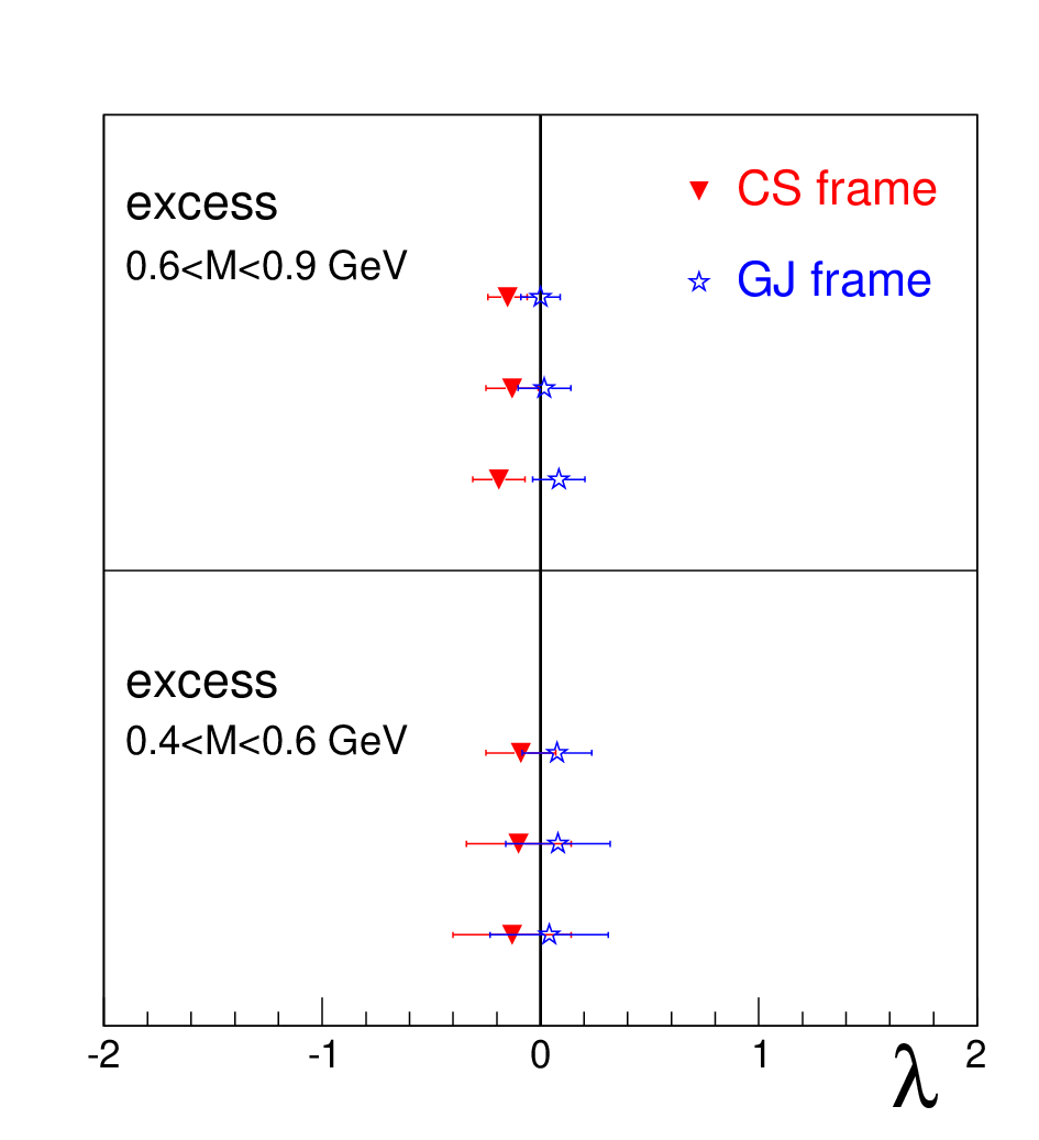
As already mentioned, once all measured, $\lambda$, $\mu$ and $\nu$ can be re-computed in any other frame. Fig. 4 shows the values of $\lambda$ and $\nu$ determined from the fits in the CS frame and in the Gottfried-Jackson frame as obtained by applying the transformation of  [6]. The structure functions remain consistent with zero independent of the frame.

The systematic error due to the combinatorial background subtraction is $\sim 2-3\%$. The systematic error due the fake matches is less than 1%. Variations in $M$, $y$ and $p_{T}$ used as input for the Monte Carlo lead to uncertainties much smaller than the statistical errors. Systematic uncertainties in the isolation of the excess range from $4-6\%$ up to $10-15\%$ in some low-populated $\cos\theta-\phi$ bins and they represent the main source of systematic errors. However, the measurement still remains dominated by the statistical errors. If the systematic errors are conservatively assumed uncorrelated from point to point and added in quadrature to the statistical fit errors quoted in the numbers above, this would increase by 15-20%.

Summarising, the absence of any polarization is fully consistent with the interpretation of the observed excess as thermal radiation. It is important to remember that this is a necessary but not sufficient condition. Put together with the other features - Planck-like shape of mass spectra, temperature systematics, agreement of data with thermal models - this makes the thermal interpretation more plausible than ever before.

References

- [1] R. Arnaldi et al. (NA60 Collaboration), Phys. Rev. Lett. 96 (2006) 162302.
- [2] R. Arnaldi et al. (NA60 Collaboration), Phys. Rev. Lett. 100 (2008) 022302.
- [3] R. Arnaldi et al. (NA60 Collaboration), Eur. Phys. J. C 59 (2009) 607.
- [4] R. Arnaldi et al. (NA60 Collaboration), Phys. Rev. Lett. 102 (2009) 222301.
- [5] K. Gottfried, J.D. Kackson, Nuovo Cimento 33, 309 (1964).
- [6] S. Falciano et al. (NA10 Collaboration), Z. Phys. C 31, 513 (1986); M. Guanziroli et al. (NA10 Collaboration), Z. Phys. C 37, 545 (1988).
- [7] A. Brandenburg, O. Nachtmann, E. Mirkes, Z. Phys. C 60, 697 (1993); D. Boer, A. Brandenburg, O. Nachtmann, A. Utermann, Eur. Phys. J. C 40, 55 (2005).
- [8] J.C. Collins, D.E. Soper, Phys. Rev. D 16, 2219 (1977).
- [9] K. Banics et al., Nucl. Instr. Methods Phys. Res., Sect. A 546, 51 (2005)