Constraining theories with Type Ia Supernovae and Gamma Ray Bursts
Abstract
Fourth - order gravity theories have received much interest in recent years thanks to their ability to provide an accelerated cosmic expansion in a matter only universe. In these theories, the Lagrangian density of the gravitational field has the form , and the explicit choice of the arbitrary function must meet the local tests of gravity and the constraints from the primordial abundance of the light elements. Two popular classes of models, which are expected to fulfill all the above requirements, have recently been proposed. However, neither of these models has ever been quantitatively tested against the available astrophysical data. Here, by combining Type Ia Supernovae and Gamma Ray Bursts, we investigate the ability of these models to reproduce the observed Hubble diagram over the redshift range . We find that both models fit very well this dataset with the present-day values of the matter density and deceleration parameters which agree with previous estimates. However, the strong degeneracy among the parameters prevents us from putting strong constraints on the values of these parameters; nevertheless, we can identify the regions of the parameter space that should, in principle, be carefully explored with future data and dynamical probes in order to discriminate among theories and standard dark energy models.
pacs
98.80.-k, 98.80.Es, 95.36.+d, 95.36.+xI Introduction
It is now widely accepted that the universe is presently undergoing a period of accelerated expansion. The Hubble diagram of Type Ia Supernovae (SNeIa) [1, 2, 3, 4, 5, 6], the anisotropy spectrum of the cosmic microwave background radiation (CMBR) [7, 8, 9] and the clustering properties probing the large - scale structure of the universe [10] are concordant pieces of evidence in favour of this cosmic speed up. In the concordance CDM cosmological model, this wide dataset is excellently reproduced [11] by assuming a spatially flat universe dominated by Cold Dark Matter (CDM) and a cosmological constant [12]. However, this scenario has two serious drawbacks: (1) if interpreted as vacuum energy, the value is 120 orders of magnitude smaller than what is expected from quantum field theory; (2) the coincidence and fine - tuning problems do not seem to have a natural explanation. This circumstance has motivated the search for alternative explanations. They mostly rely on scalar fields with a suitable potential which provides a varying term or other dark energy fluids [13] with exotic properties.
An alternative route towards solving the problem of the accelerated cosmic expansion may be explored by looking at the cosmological constant as an additive constant term in the Einstein - Hilbert gravity Lagrangian: from the point of view of the field equations, one is not adding any new source term to the energy-momentum tensor, but rather it is the geometrical sector (the left-hand side of the equations) that has been modified. It is therefore worth wondering whether the accelerated expansion can indeed be obtained by generalizing this approach, i.e. by adding other non - linear terms to the action. The search for a generalization of Einstein General Relativity (GR) actually dates back to just few years after the seminal Einstein papers (see, e.g., [14] for a historical review), but the relevance of these corrective terms were considered to be restricted only to the strong gravity regimes. Moreover, effective field theory considerations motivated the introduction of small couplings which suppress these non - linear terms in all the other curvature regimes. As a consequence, corrections to GR were considered only close to the Planck scale, i.e. in the very early - universe [15], and in the attempt to avoid black hole singularities [16].
The qualitative similarities between the present - day acceleration and the early universe inflationary expansion renewed the interest in what are now collectively referred to as theories. Indeed, it became clear soon that an accelerated expansion in a matter only universe can be achieved by suitably choosing the functional expression for leading to a non-linear gravity Lagrangian, . The impressive amount of papers [17, 18] investigating different aspects of theories helps understanding that the success in explaining the cosmic acceleration must be balanced by the constraints provided by the local gravity tests (see, e.g., [19] for exhaustive reviews discussing these issues). Indeed, many models providing an accelerated expansion were later rejected because the non-linear terms do not turn off their effect on the Solar System scale and thus lead to unacceptable contrast with the success of GR in this regime.
Recently, two models carefully designed to evade the local gravity tests but still providing an accelerated cosmic expansion has been proposed [20, 28]. However, neither of these models has yet been quantitatively tested against the available astrophysical data. Here, in order to to further support (or rule out) theories as alternative candidates to the dark energy hypothesis, we search for the appropriate set of parameters of these models to verify that the acceleration, that they qualitatively predict, actually quantitevely agree with the data.
The scheme of the paper is as follows. In § II, we will briefly remind the basics of theories writing down the equations needed to determine the background evolution of the universe. § III discusses the theoretical constraints driving the choice of a functional expression for thus motivating the adoption of the two popular models to be tested. The data used and the statistical method used to constrain the model parameters are presented in § IV, while the results of the analysis are commented upon in § V. Conclusions and future perspectives are finally given in § VI.
II cosmology
The idea of modifying the gravity sector of the Einsteinian General Relativity (GR) dates back to the Starobinsky [15] attempts to get an inflationary expansion of the early universe without the need of any scalar field. This can be accomplished by generalizing the Einstein - Hilbert action as :
| (1) |
where is the scalar curvature, (we use units where the light speed ), is the standard matter Lagrangian, and is an analytical function expressing the deviation from the Einstein GR. For , we get back the concordance CDM model, while nontrivial dynamics is obtained for other choices.
Under the metric approach to gravity, the field equations are obtained by varying the action (1) with respect to the metric only. We obtain :
| (2) |
with and the usual Einstein and source stress - energy tensor. Hereafter the subscript will denote differentiation with respect to . We also assume a spatially flat Robertson - Walker metric, with scale factor ; in this case, the scalar curvature reads
| (3) |
where is the Hubble parameter and the dot indicates the time derivative; by using the more convenient variable , we denote the derivative with respect to with a prime. With these definitions, Eqs.(2) lead to the modified Friedmann equation
| (4) |
where we have assumed that dust matter with enery density and pressure is the only fluid filling the universe. To solve Eqs.(3) and (4), we follow [20] and introduce the dimensionless variables :
| (5) |
with
| (6) |
a convenient curvature scale depending on the present day values of the matter density parameter and the Hubble constant . The background evolution of the universe is determined by the following set of coupled ordinary differential equations :
| (7) |
| (8) | |||||
It is worth noting that the above system of equations of first order in is equivalent to a single second order equation in . If we look at the definition of , we see that the full system is equivalent to a single fourth-order non-linear differential equation for the scale factor : this property explains why theories are also commonly referred to as fourth-order gravity theories.
In order to integrate the system, we need to set the boundary conditions. In [20], the authors set them at redshifts , by requiring that tends to a constant at this epoch and by considering the detailed balance of the perturbative corrections to . However, here we are interested in fitting the model to data that probe the range ; therefore, it is more interesting to set the present day values of and integrate the equations back in time up to . By setting, as usual, and remembering that
| (9) |
with the deceleration parameter, we get:
| (10) |
It is worth noting that, because of Eq.(6), the initial conditions (10) are determined by the values of the three parameters . This is again consistent with models being fourth-order theories; thus, we require three initial conditions to determine the evolution of the scale factor for any given . Had we written down a single equation for , we should have set the present - day values of the first three time derivatives of which include the jerk parameter . In contrast, the introduction of the auxiliary functions and of the curvature scale enables us to replace the quite uncertain jerk parameter with the more manageable matter density .
III models
A key role in fourth - order gravity is obviosuly played by the functional expression of . In principle, such a choice is fully arbitrary unless one has a theoretical motivation leading to a unique expression for . Actually, things are not so easy. Indeed, the modification of GR introduces deviations not only on the cosmological scales, but at all the scales where gravitational phenomena can be tested. In particular, it has proven to be quite difficult for a large class of theories to evade the constraints on the Solar System scale (see, e.g., [21] and refs therein). As Chiba [22] has shown, the main difficulty arises from models introducing a new scalar degree of freedom with the same coupling to matter as gravity. As a consequence, it appears a long range fifth force that violates the constraints on the PPN parameters. Although the derivation of the PPN parameters has been questioned [23], significant deviations from the GR metric around the Sun seem to be confirmed because of a decoupling of the scalar curvature from the local density. As a possible way out, one can invoke a chamaleon effect [24] to reassociate high density with high curvature so that the scalar degree of freedom becomes very massive and the fifth force escapes any detection. To this aim, should be tailored in such a way to give rise to a mass squared term which is large and positive in high curvature environments [25]. It is worth stressing that this same condition is also required if we want to recover GR in the early universe [26] and obtain the usual matter dominated era. Since in this limit, we expect that tends to a small constant in order to make its effect negligible with respect to the GR term. On the other hand, in the late universe, we expect to mimic the same evolutionary history of the CDM because this model agrees with the data; therefore should reduce again to a small constant, but it should again tend to zero in the limit of a vanishing to agree with the observational fact that takes a very low value. Summarizing, one has to look for a functional expression satisfying the following constraints:
| (11) |
where is a typical curvature scale and the last condition [27] ensures that, in the limit , the solution is stable at high curvature.
Among the possible choices left out by the above conditions, we will consider here two classes of models. For the first one, we follow [20] and set:
| (12) |
with given by (6), and are positive dimensionless constants. We will refer to this choice as the Hu & Sawicki (hereafter, HS) model by the name of the authors who first suggested this expression. It is easy to check that all the constraints (11) are easily passed by the HS model. In particular, we note that, since , there is no actual cosmological constant in the model, but
so that, when at fixed , we recover an effective cosmological constant in high curvature environments.
Another possibility to satisfy all the constraints (11) is offered by the Starobinsky proposal [28] :
| (13) |
with a scaling curvature parameter and two positive constants. We will refer to this class of theories as the Starobinsky (St) model. Note that, even in this case, so that no actual cosmological constant is present. Nevertheless, an effective one is recovered in the high curvature regime as can be seen from with .
As a general remark, we note that the HS and St models are quite similar at both very low and very high redshifts since they are both built up by imposing the same constraints on . Moreover, they both aim at mimicking the successful CDM scenario in the late and early universe. Put in other words, the HS and St models both reduces to the GR + case in the limits of very high and very low curvature. What makes them different is the way the two extreme cases are connected, i.e. how the universe evolves from the present day dominated phase to the early matter epoch.
For completeness, we finally remind the reader that the two models we are considering here are not the only viable ones; other possible examples are given in [29, 30]. It is, moreover, possible to work out models which can also provide an inflationary expansion in the very early universe [31]. However, all these other cases share many similarities with the HS and St models so that we are confident that exploring just two classes of fourth-order gravity theories should provide us with some general conclusions on their viability.
IV Constraining the models
Any model that aims to describe the evolution of the universe must be able to reproduce what is indeed observed. Matching the model with observations is also a powerful tool to constrain its parameters and allows to estimate some further quantities of interest.
As mentioned above, the HS and St models are carefully designed to give an effective cosmological constant in the late universe. Moreover, both theories are assigned by a three parameters function, and one can anticipate that the considerable freedom allowed by the degeneracy among the parameters makes it easy to find some combinations that lead to quite similar in the low regime. Fitting to SNeIa data can only tell us whether the models are viable over the redshift range . We expect that this is indeed the case because the functions have been tailored to do so. What is not garanteed is that the HS and St models can describe the background expansion up to higher redshifts . To probe this regime, we will use the recently derived Hubble diagram of Gamma Ray Bursts (GRBs).
In the Bayesian approach to model testing, we explore the parameter space through the likelihood function :
| (14) | |||||
where p denotes the set of model parameters. Before discussing in detail the term related to the SNeIa and GRB data, we concentrate on the two Gaussian priors. The former takes into account the constraints on the physical matter density with
as inferred from WMAP5 data [9]. One can wonder whether such an estimate may be used as a constraint on the models since it has been obtained by fitting the CMBR spectrum assuming the validity of GR. However, what is really needed for this estimate to be model independent is not that GR holds along all the evolutionary history, but that the gravity Lagrangian reduces to the Einstein - Hilbert one at the last scattering. Since, for both HS and St models, for , we can safely use the WMAP5 value as a constraint.
The Gaussian prior on in Eq.(14) stems from the results of the HST Project [32] which has estimated the Hubble constant using a well calibrated set of local distance scale. Averaging over the different methods, the survey finally gives :
as a cosmological model independent constraint11 1 While this work was near completion, the SHOES collaboration [33] has released a more precise estimate as in agreement with our adopted value..
The main two terms in the likelihood (14) are both related to the Hubble diagram, the first one being, in particular, connected with SNeIa. These latter data have provided the first piece of evidence for the cosmic speed up and are still a sort of ground-zero test that every cosmological model has to pass to be considered acceptable. To check this, one relies on the predicted distance modulus :
| (15) |
with the dimensionless comoving distance :
| (16) |
The likelihood function is then defined as
| (17) | |||||
where is the total number of SNeIa used, is a - dimensional vector with the values of and is the covariance matrix of the SNeIa data. Note that, if we neglect the correlation induced by systematic errors22 2 Actually, it has been shown [34] that neglecting systematic errors does not shift the central values, but only weakens the constraints. Although such a result has been obtained using standard dark energy models, we are confident that this is also the case for our theories., as we do here, is a diagonal matrix and Eq.(17) simplifies to :
| (18) |
with
| (19) |
with the error on the observed distance modulus for the i - th object at redshift . As input data, we use the Union SNeIa sample assembled in [34] by reanalysing with the same pipeline both the recent SNeIa SNLS [4] and ESSENCE [5] samples and older nearby and high redshift [3] datasets.
Although quite useful in probing the accelerated expansion, SNeIa are limited to . As a consequence, one has to resort to a different distance indicator to push the Hubble diagram to higher redshift and probe the (supposedly) matter dominated era. Thanks to the enormous energy release that makes them visibile up to , GRBs stand out as ideal candidates to this scope. The discovery of 2D correlations between their properties have opened the way towards making GRBs standard candles similarly to SNeIa [36]. As a result, Schaefer [35] have provided the first GRBs Hubble diagram containing 69 objects with estimated by averaging over 5 different 2D correlations. We use here the updated GRBs Hubble diagram recently presented in [36] based on a model-independent recalibration of the same 2D correlations used by Schaefer.
Since there is no correlation among the errors of different GRBs, the likelihood function now simply reads :
| (20) |
with
| (21) |
where takes care of the intrinsic scatter inherited from the scatter of GRBs around the 2D correlations used to derive the individual distance moduli.33 3 Note that a similar term is also present for SNeIa, but it is estimated to be and yet included into the error provided in the Union dataset.
V Results
The functions for the HS and St models in Eqs.(12) and (13) depend on three parameters, while other three parameters are needed to set the initial conditions (10). By adding the GRBs intrinsic scatter , we end up with a seven dimensional parameter space to be explored. To do this efficiently, we use a Markov Chain Monte Carlo code which maximizes the likelihood (14) along a chain with points. The constraints on the parameters are then obtained by cutting out the first of the chain; we thus skip the burn-in phase and thin the chain to reduce spurious correlations.
Before discussing the results, we warn the reader that, in the context of Bayesian statistics, the best fit model, i.e, the set of parameters maximizing , represents the most plausible model in an Occam’s razor sense given the data at hand. However, in a Bayesian context, the best fit parameters individually do not necessarily have to be probable, but rather they must have a high joint probability density that might occupy only a small volume of the parameter space. This situation can arise if the best fit solution does not lie in the bulk of the posterior probability distribution. Such a situation may often occur when the posterior is non-symmetric in a high dimensional space so that the volume can dramatically increase with the distance from the best fit solution. In this case, the best fit solution for each parameter could easily lie outside the bulk of the individual posterior distribution for obtained by marginalizing over the other parameters. This is indeed what happens for our models so that we have preferred to remind the reader that this somewhat counterintuitive outcome is not a problem, but rather a common feature in statistics in multi-dimensional spaces.
V.1 The HS model
The HS functional expression depends on three dimensionless positively defined parameters. While it is reasonable to expect that is not a large quantity, nothing can be said a priori on the order of magnitude of . Indeed, should both of them be very large, then eq. (12) reduces to so that this case provide an effective cosmological constant. In contrast, should be very small, we get thus recovering power - law corrections to the Einstein - Hilbert Lagrangian which are known to provide accelerated expansions for . We must therefore explore a huge range for ; we thus skip to logarithmic units and get constraints on by running the MCMC code.
The best fit model turns out to be :

with a best fit GRB intrinsic scatter . The overall quality of the fit may be seen by looking at Fig. 1 and quantified by considering the following estimators :
so that we can safely conclude that the HS model is in very good agreement with the data. A cautionary note is in order here concerning the values reported above. The MCMC code maximizes the likelihood (14) which is strictly not the same as minimizing either or . Moreover, from a statistical point of view, the significance level of the above reduced values can not be estimated from the usual tables since these standard results do not take into account systematic errors or intrinsic scatter. As such, both and must be considered only as a useful tool to quantify the agreement with the data, but should not be overrated.
The constraints on the single parameters are summarized in Table I where we give the mean and median values and the and confidence limits. While the best fit solution for is quite close to the median values, this is not the case for , with the best fit solution for lying marginally outside the CL. However, according to the Bayesian philosophy, one must take the constraints in Table I as the final outcome of the likelihood analysis. It is, however, worth noting that setting all the parameters to their median values gives :
so that the quality of the fit is still not unreasonably bad.
| CL | CL | ||||
|---|---|---|---|---|---|
| 0.282 | 0.282 | 0.282 | (0.268, 0.296) | (0.256, 0.309) | |
| 0.703 | 0.700 | 0.700 | (0.692, 0.708) | (0.685, 0.716) | |
| -0.67 | -0.63 | -0.62 | (-0.70, -0.55) | (-0.88, -0.45) | |
| 4.26 | 2.52 | 2.36 | (1.84, 3.24) | (1.44, 4.21) | |
| -0.53 | 1.15 | 1.00 | (-1.07, 2.96) | (-2.31, 7.12) | |
| -8.39 | -7.64 | -7.65 | (-9.23, -6.11) | (-9.90, -5.27) | |
| 0.41 | 0.29 | 0.29 | (0.17, 0.41) | (0.03, 0.50) |
In order to further investigate the viability of the model, we can compare the constraints on with other results in the literature.44 4 We no longer consider anymore the Hubble constant because this is typically marginalized over when fitting Hubble - diagram data because of the degeneracy with the (unknown) SN absolute magnitude. Such a degeneration is partially broken here thanks to the use of two different distance indicators and the Gaussian prior from the HST Key Project; however, we prefer not to discuss the corresponding constraints because other model independent estimates in the literature (coming from, e.g., time delays in multiply lensed quasars) are affected by too large uncertainties. However, the matter density parameter is always estimated by fitting a given model to a certain set of data so that a straightforward comparison may be biased by the different theory we are considering. Therefore, we simply note that the values in Table I are in very good agreement with typical estimates [6, 34, 9] from previous analyses of comparable datasets.
Something more interesting can be said on the deceleration parameter . Indeed, the problem of model dependent estimates can now be avoided by resorting to cosmographic analyses based only on the Taylor expansion of the scale factor. By using this approach, Cattoën and Visser [37] have found values between and , depending on the details of the method used to fit the SNLS dataset. A similar analysis, but using a different and smaller GRBs sample, enabled Capozziello and Izzo [38] to find values between and , still in agreement with our estimates. A different approach has been instead adopted by Elgarøy and Multamäki [39] which advocate a model-independent parametrization of . Depending on the SNeIa sample used and the parametrization adopted, their best fit values for range between and still in good agreement with our constraints in Table I.

While the value of tells us that the model is nowadays undergoing accelerated expansion, it is also important to check that this cosmic speed up ends well before the epoch of structure formation. To do so, for each point along the Markov chain, we compute the deceleration parameter and solve the equation with usually referred to as the transition redshift. We then make a histogram of the values and use this as a proxy for its probability distribution so finally estimating :
These constraints may be compared with previous results. For instance, by using the Gold SNeIa sample and linearly expanding , Riess et al. [3] found in agreement with the updated result obtained by Cuhna [40] which use the Union sample. Although there is a very good agreement, we nevertheless warn the reader that the estimate of is strongly model dependent. To be conservative, we may therefore only conclude that the transition to a decelerated epoch in the HS model takes place early enough not to conflict with the growth of structures and galaxy formation.
Although no previous analysis of the HS model has been performed, it is worth considering the constraints on the parameters . The first striking result is the very high value of with being, in contrast, very low. Unless we are in the early universe when also takes a very high value, the bulk of the models with in Table I, the HS gravity Lagrangian may be approximated as :
with the low value of compensating for the large so that the two terms and are comparable. From Table I, we also get so that the likelihood analysis is selecting a subclass of the HS model that behaves as if the gravity Lagrangian were in the late universe.
In a sense, such a result could be anticipated by remembering the history of fourth order gravity theories. Indeed, as quoted above, the first successfull model was proposed by Starobinsky in the ’80s to give an accelerated expansion by adding a quadratic term to the Einstein - Hilbert Lagrangian, i.e. setting . Indeed, the HS reduces to the Starobinsky inflationary model for and with weighting the relative importance of the two terms and . Indeed, by looking at the likelihood contours in the plane shown in Fig. 2, one can see that, for a given value, there are two solutions, depending on the being larger or smaller than 2. For , the solution with the smaller provides a better fit to the data. In this regime, one gets that the more weight one gives to the corrective term, the more accelerated is the present day expansion. It is therefore not surprising that our likelihood analysis has indeed converged not too far from the inflationary model.
We stress, however, that, even with and , the HS model remains fundamentally different from the Starobinsky inflationary model. Indeed, the accelerated expansion is now obtained at the present day rather than in the early universe. For very high , has become so large that the term in the denominator of Eq. (12) is dominant and we recover the limit , i.e. an effective cosmological constant. Moreover, it can be shown that, although large, this constant term is nevertheless negligible with respect to so that we fully recover the GR Lagrangian and we do not thus violate the constraints from BBN and the abundance of primordial light elements.
V.2 The St model
As for the HS case, the expression (13) of the St model still is a function with three parameters, namely . It is, however, convenient to reparameterize the model in terms of dimensionless quantities. To this aim, we first define :
| (22) |
with the present day scalar curvature so that Eq.(13) becomes :
| (23) |
Concerning the values of the two parameters , we can only have some hints on what their order of magnitude can be. To this aim, we first note that , with an unknown reference redshift. A plot of for a fiducial CDM model shows that this ratio can easily take very large values even at intermediate redshift. Needless to say, the St model is not the CDM one, but we can anticipate that, in order to fit the data, its expansion rate will not differ much so that will take similar values. As a result, we therefore end up with taking high values so that we skip to as a parameter to be constrained by the MCMC analysis. To get an idea of the range for , we note that, in the early universe, the Lagrangian reduces to :

so that . Since we want to recover the GR in this limit, we just have to ask that . However, this ratio can easily be very small even if is quite high so that we end up with varying over a wide range. Therefore, we skip again to logarithmic units taking as a model parameter.
Running the MCMC gives us as best fit parameters :
with a best fit GRB intrinsic scatter . The values of the reduced and of
| CL | CL | ||||
|---|---|---|---|---|---|
| 0.283 | 0.278 | 0.277 | (0.260, 0.295) | (0.247, 0.308) | |
| 0.704 | 0.705 | 0.705 | (0.694, 0.716) | (0.686, 0.728) | |
| -0.78 | -0.79 | -0.78 | (-0.97, -0.61) | (-1.16, -0.52) | |
| 1.44 | — | — | |||
| 1.56 | 1.03 | 1.05 | (0.53, 1.48) | (0.24, 1.94) | |
| 2.86 | 2.68 | 2.67 | (1.51, 3.91) | (0.89, 4.42) | |
| 0.38 | — | — |
clearly show that the best fit St model is in very good agreement with the data as can also be appreciated by looking at Fig. 3. Table II reports mean, median and confidence ranges for the individual parameters. An important caveat is in order here for the parameters and . Indeed, the Markov chain tends to drift towards negative values of which are a priori excluded in order the St model to pass the theoretical constraints (11). Therefore, the histogram of values is clearly cut by this a priori assumption and, although formally mean and median values may be computed, they are not reliable. We thus give only upper limits on because the data are unable to constrain this model parameter. A similar problem also takes place for the intrinsic scatter which must be positive by definition. Nevertheless, the chain drifts towards the border probably because of a degeneration with , with low preferring low scatter. We therefore only give upper limits on too.
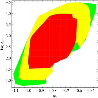
The comparison between Table I and II shows that the values of the three parameters are consistent with each other. There is actually some tension for the deceleration parameter with the St model favouring a greater speed up, but the good overlap of the confidence ranges makes this difference statistically irrelevant. We do not discuss the comparison with previous results in the literature but we refer to what we have said above for the HS model. As a remark, however, we note that the agreement of the parameters is not completely unexpected. Indeed, these quantities set the initial conditions (10) so that this is only telling us that the auxiliary functions are very close to each other for . Since both the HS and St models are designed to fit the same present day data, it is not surprising that they are quite similar today and lead to the same values of the parameters which set the initial conditions.
It is, on the contrary, somewhat surprising that, notwithstanding the initial larger acceleration, the transition redshift (estimated with the same procedure used above) is lower than in the HS case, being :
Although formally in marginal disagreement at the level with the results for the HS model, the two sets of constraints are however not too different. In particular, the St value remains in good agreement with the previous estimates in the literature.
Finally, even if we cannot put strong constraints on , we briefly discuss their values. First, we note that, since the term quickly starts dominating over unity, at intermediate , we get :
Let us suppose, for a moment, to drop the assumption . Indeed, for , the above is approximated by the sum of a (negative) cosmological constant and a quadratic correction modulated by the value of . Once again, we therefore recover a Lagrangian similar to the inflationary Lagrangian of Starobinsky, since the negative cosmological constant soon becomes subdominant. This qualitative discussion helps us understanding why the chain drifts towards negative which have been excluded, in order to give Eq.(13) the correct limit for . For , the code is forced to look for an accelerating solution in this regime. Since, again, the term quickly overcomes the unity, the above approximation of the St still holds; we may easily note that the dominant correction is of the form so that the best fit makes the model similar to the proposal firstly introduced as a fourth - order gravity motivated alternative to scalar field dark energy. As a final remark, we look at Fig. 4 which shows that is correlated with the weighting parameter which here plays the same role as for the HS model.
V.3 The effective dark energy EoS
The impact of on the expansion history can be alternatively discussed by resorting to the effective dark energy equation of state (hereafter, EoS). Indeed, from the point of view of the background evolution, models are equivalent to a cosmological scenario made out of dust matter and an effective dark energy term with an EoS given by :
| (24) | |||||
so that the dark energy density parameter reads :

| (25) |
Fig. 5 shows the effective EoS for both the HS and St models setting the parameters to their best fit values. It is impressive to see how closely the two EoS are with being almost exactly the same for the two models for . Note that here we have not plotted the full redshift range up to the last scattering to make easier to see the details at low . However, when , we have checked that converges to , i.e. the effective dark energy behaves as a matter term in the early universe and scales with the redshift in the same way. This is still an expected consequence of the constraints (11) ensuring that for . In such a limit, we therefore recover a GR universe with only matter. Hence, we get which, inserted into Eq.(24) leads to whatever is the model considered.
The HS and St effective EoS are different in the low regime. Indeed, for the best fit models, we find :
for the HS model and :
for the St case. For both models, the present day values of and its redshift derivative disagree with the CDM expected values, and . Actually, we must consider the Bayesian constraints obtained from evaluating these quantities along the chain. For , we find :
for the HS model, while for the St we get :
Defining , we get :
for the HS model, while in the St case it is :
As it is apparent, an effective cosmological constant is reasonably consistent with these constraints. The present day value of the EoS is indeed close to , while its first derivative, although being not null, is quite small and consitent with zero within the confidence range. However, we stress that neither the linear fit nor the widely used Chevallier - Polarski - Linder [43] ansatz provide a good approximation over the redshift range probed.
As a final remark, let us look again at Fig. 5. For both theories, the effective EoS takes a positive value during the epoch of galaxy formation and over a wide redshift range in the matter dominated epoch. However, the effective dark energy density is very small during this period so that the deceleration parameter stays almost constant to for as for a matter only universe. It is, therefore, likely that the departures from have essentially no impact on the background when struture formation takes place.
V.4 Local tests of gravity
The functional law for both the HS and St models has been formulated in such a way to pass the constraints (11). However, this does not mean that there are no detectable deviations from the GR metric on Solar System and galactic scales whatever the model parameters are. Indeed, the HS and St models correctly represent two different classes of theories containing, as particular cases, models which are able to evade the local tests of gravity. It is therefore interesting to explore whether the cosmologically selected models belong to this subclass. A key role will be played by the value of . By evaluating this quantity along the chain, we get :
for the HS model and
for the St model.
In order to see how these values compare with the constraints from the local tests of gravity [41], we follow [20] who have explicitly considered the case of the HS model. They have demonstrated that, in order to be consistent with the constraints on the PPN parameter , one has to impose the following condition :
| (26) |
Such a constraint thus depends on the value of the HS model parameters and could, in principle, be included to limit the volume of the parameter space to be explored. However, we have preferred to let the MCMC code be free of searching the full parameter space since (26) is actually a quite weak prior. Indeed, for the best fit model, this reduces to , while the best fit value is so that the test is easily passed.
Unfortunately, we are unable to impose a similar constraint to the St model. To this aim, one should first solve the field equations for a static spherically symmetric source matching the inner and outer solutions and taking care of a model for the Sun mass density profile. In [20], it is argued that, for every model, the PPN parameter may always be expressed as,:
with the total solar mass and
with and the scalar curvature of the local metric as function of the radial coordinate and the mass density profile. In order to pass the Solar System constraints, should be as low as possible which can be accomplished by making follow so that a chamaleon effect takes place. Since the St model has been designed in such a way to develop such an effect, we are confident that the Solar System constraints are fulfilled even if we cannot make any quantitative estimate.
Finally, let us consider the galactic scales where the following constraint
| (27) |
where is the maximum rotation velocity of the stars, has been advocated in [20] as a indepedent condition to be fulfilled in order to have no deviations of the gravitational potential from the Keplerian profile on the galaxy scales. We remind that [20] look for a model describing the accelerated expansion of the Universe, but still require a substantial dark matter content. However, the leading term of the Lagrangian of our best fit models induce a power law deviation from the Newtonian gravitational potential which was shown to describe the rotation curves of dwarf galaxies without the need of dark matter [42]. Therefore, it is not surprising that our cosmologically motivated constraints on are definitively larger than the upper limit for a Milky Way like galaxy. Although the result of the Lagrangian used by [42] cannot be directly extrapolated to the HS and St models, it is however suggestive that the violation of Eq.(27) is an expected outcome of the region in the parameter space preferred by the data.
Rotation curves of spiral galaxies are an excellent probe of the gravitational potential so that we can rely on them to judge whether any deviation from the classical Newtonian result is detected. Indeed, the observed flatness of in the outer regions, well far away from the edge of the visible disc, clearly indicates that something unusual is taking place. If one assumes a priori that the potential remains Keplerian even on these scales, the only solution is to invoke the presence of a halo made out of dark matter particles (which have not yet directly observed). In contrast, one can reject the dark halo hypothesis and thus interpret the flateness problem as an evidence for deviations from the Newtonian potential. Should this interpretation be correct, one can try to fit the rotation curves with a modified potential coming out of the low energy limit of a theory, which has indeed been done with success [42]. As such, the fact that both the cosmologically selected subclasses of the HS and St models violate the constraint (27) should not be considered as a serious problem. Actually, giving off the dark halo in favour of a modified potential could lead to a different problem. In such a case, indeed, the matter density parameter should reduce to the baryons only one, i.e. in disagreement with the values in Tables I and II. A possible way out could be to invoke massive neutrinos [45] or a dark matter component only present on cluster scales.
As a final remark, however, it is also possible that the constraint (27) is overrestrictive or not valid at all. Indeed, Eq.(27) has been obtained assuming a spherical galaxy described by an NFW [44] profile. Such a profile is motivated by numerical simulations which assumes the validity of GR and hence a Newtonian gravitational potential. Therefore, testing the validity of GR based on a model which yet assumes this is the case is somewhat a contradiction. Moreover, the derivation in [20] assumes that the galaxy is an isolated system, while galaxies actually reside in groups or clusters. Should a long range fifth force be present, its effect must be taken into account when deriving a constraint in Eq.(27). As a consequence, an analytical computation which takes care of all these details is likely to be impossible and one should resort to N - body simulations in a cosmological background, which are yet unavailable. Because of these problems, we warn the reader against considering the violation of (27) by the HS and St models as a definitive evidence that these theories should be ruled out.
VI Conclusions
As soon as the observational and conceptual problems related to the cosmological constant and other dark energy scenarios became pressing, modification of the gravity sector of Einstein field equations immediately appeared as an interesting alternative explanation of the observed cosmic speed up. Fourth - order gravity theories then appeared as the most immediate generalizaton of Einstein GR since they just encoded all the deviations into a single analytic function . As the problem of acceleration was solved in this framework, a new problem came out, namely how to choose a functional expression for which is not only able to speed up the expansion (there were too many actually!), but also not to violate the local tests of gravity and turn off its effect in the early universe where GR indeed correctly appears to work.
From a mathematical point of view, one has to look for a expression satisfying the constraints (11) which is indeed what the HS and St models efficiently do, postulating that is given by Eqs.(12) and (13), respectively. Our aim here was then to test whether these two well behaved models actually fit the data which suggest the accelerated expansion of the Universe. To this end, we have considered the background evolution as probed by the Hubble diagram by using both SNeIa and GRBs to cover the redshift range . As a first encouraging result, it turns out that both the HS and St models are in very good agreement with the data. Moreover, the predicted values of the matter density parameter , the Hubble constant , the deceleration parameter and the transition redshift nicely compare with previous estimates in the literature. As a further positive outcome, the cosmologically selected subclasses of the general HS and St parameterizations easily pass the constraints on the PPN parameter and reduce to GR in the early universe, as can also be seen by noting that the corresponding effective EoS and density parameter vanish at the redshift of the last scattering surface. Some unpleasant tension with the constraints on the deviation from the Newtonian potential on galaxy scales is possible, but the way these constraints are derived put serious doubts on their validity hence decreasing the significance of the problem.
While this manuscript was near completion, a paper was posted on the arXiv [46] where the authors try to constrain the HS model parameters using the Union SNeIa sample, the Hubble expansion and age data [47] and the Baryonic Acoustic Oscillations [48]. However, their results may not be compared straightforwardly to ours in Table I. Notwithstanding the different dataset used, the main difference relies in how they reparameterize the HS model. While we have directly used as parameters, they prefer to use the set with the effective matter density parameter and estimated by :
Finally, they have limited a priori their exploration of the parameter space to models with , while we have shown here that the best fit is obtained for much larger values. In principle, we can solve the above relations to get for our best fit model. But this is actually not possible since such relations have been obtained assuming that which is not true in our case. Such a condition was also imposed in order to have not departing too much from a cosmological constant, but we have shown here that this is an unnecessary assumption. Indeed, for both the HS and St models is close to the EoS over a very limited range, but nevertheless we are able to fit the data since the impact of the effective dark energy term becomes quickly subdominant during the matter dominated era no matter what its EoS is.
As Fig. 5 shows, although the functional expression is different, both the HS and St best fit models have a very similar effective EoS and hence the predicted distance modulus is almost the same. Moreover, the values in Tables I and II tell us that the SNeIa and GRBs Hubble diagram is unable to put strong constraints on the model parameters.
It is worth wondering how the situation can be improved. As a first attempt, one can try to extend the redshift range probed by relying on the use of the so-called distance priors [9, 49] which provide a useful set of distance-related quantities that summarize the information contained in the CMBR anisotropy spectrum. Although widely used as observational constraints in the recent literature [50], it is worth stressing that they are derived by assuming a fiducial CDM model. It is then argued that the mean and covariance matrix of the distance priors parameters do not change when the model space is enlarged, i.e. the choice of the fiducial model does not impact the estimate of the priors. Moreover, one also assumes that the posterior probability from the CMBR anisotropies and galaxy power spectra is correctly described by the distance priors, i.e. no information is lost when dropping the full dataset in favour of the simplified one. While both these hypotheses have been verified for dark energy models [51], such an exercise has never been performed for theories. Therefore, to be conservative, we have preferred not to use them in the present analysis. One can, however, argue that including the distance priors can narrow down the constraints on some of the model parameters, but it is likely that the degeneracy between the HS and St models is not broken. Indeed, the distance priors probe the universe mainly at the last scattering redshift thus complementing SNeIa and GRBs which cover the range . However, in the early universe, both the HS and St models converge to GR so that they are likely to be too similar to be discriminated by probing this redshift regime.
Major improvements in the constraints and in the possibility to discriminate not only between the HS and St models, but, more generally, among dark energy and theories are expected from the analysis of the growth of perturbations. Indeed, even if one can tailor the parameters in order to closely mimic the same expansion history of a given dark energy model, the evolution of the density perturbations can be rather different [27, 52, 53]. In particular, this has a strong impact on both the power spectrum and halo statistics [54] and the weak lensing signals [55]: it is thus possible to compare predictions with data and severely constrain the viability of theories.
It is this combination of extended Hubble diagrams (made out of SNeIa and GRBs) and structure growth probes (such as galaxies power spectrum and cosmic shear) that will finally tell us whether the observed cosmic speed up has been the first evidence of a new fluid, as mysterious as fascinating, or of new physics in the gravity sector, as unexpected as challenging.
Acknowledgements.
VFC warmly thanks S. Capozziello and M.G. Dainotti for their collaboration in getting the GRBs Hubble diagram and V. Salzano for assistance with the Markov chains. VFC is supported by University of Torino and Regione Piemonte. The authors also ackwnoledge partial support from INFN grant PD51.References
- [1] S. Perlmutter et al., ApJ, 483, 565, 1997; A.G. Riess et al., AJ, 116, 1009, 1998; B.P. Schmidt et al., ApJ, 507, 46, 1998; P.M. Garnavich et al., ApJ, 509, 74, 1998; S. Perlmutter et al., ApJ, 517, 565, 1999
- [2] R.A. Knop et al., ApJ, 598, 102, 2003; J.L. Tonry et al., ApJ, 594, 1, 2003; B.J. Barris et al., ApJ, 602, 571, 2004
- [3] A.G. Riess et al., ApJ, 607, 665, 2004; A.G. Riess et al., ApJ, 659, 98, 2007
- [4] P. Astier et al., A&A, 447, 31, 2006
- [5] W.M. Wood - Vasey et al., ApJ, 666, 694, 2007
- [6] T. Davis et al., ApJ, 666, 716, 2007
- [7] P. de Bernardis et al., Nature, 404, 955, 2000; R. Stompor et al., ApJ, 561, L7, 2001; C.B. Netterfield et al., ApJ, 571, 604, 2002; R. Rebolo et al., MNRAS, 353, 747, 2004
- [8] C.L. Bennett et al., ApJS, 148, 1, 2003; D.N. Spergel et al., ApJS, 148, 175, 2003 D.N. Spergel et al., ApJS, 170, 377, 2007
- [9] E. Komastu et al. 2009, ApJS, 180, 330, 2009
- [10] S. Dodelson et al., ApJ, 572, 140, 2002; W.J. Percival et al., MNRAS, 337, 1068, 2002; A.S. Szalay et al., ApJ, 591, 1, 2003; E. Hawkins et al., MNRAS, 346, 78, 2003; A.C. Pope et al., ApJ, 607, 655, 2004
- [11] M. Tegmark et al., Phys. Rev. D, 69, 103501, 2004; U. Seljak et al., Phys. Rev. D, 71, 043511, 2005; M. Tegmark et al., Phys. Rev. D, 74, 123507, 2006
- [12] S.M. Carroll, W.H. Press, E.L. Turner, ARAA, 30, 499, 1992; V. Sahni, A. Starobinski, Int. J. Mod. Phys. D, 9, 373, 2000
- [13] P.J.E. Peebles, B. Rathra, Rev. Mod. Phys., 75, 559, 2003; T. Padmanabhan, Phys. Rept., 380, 235, 2003; E.J. Copeland, M. Sami and S. Tsujikawa, Int. J. Mod. Phys. D, 15, 1753, 2006
- [14] H.-J. Schmidt, ECONF C0602061, 12, 2006
- [15] A.A. Starobinsky, Phys. Lett. B, 91, 99, 1980
- [16] R. H. Brandenberger, arXiv : gr-qc/9210014, 1992; R. H. Brandenberger, arXiv : gr-qc/9302014, 1993; R. H. Brandenberger, arXiv : gr-qc/9509059, 1995; V. F. Mukhanov and R. H. Brandenberger, Phys. Rev. Lett. 68, 1969, 1992; R. H. Brandenberger, V. F. Mukhanov, and A. Sornborger, Phys. Rev. D48, 1629, 1993; B. Shahid-Saless, Journal of Mathematics and Physics 31, 2429, 1990; M. Trodden, V. F. Mukhanov, and R. H. Brandenberger, Phys. Lett. B316, 483, 1993
- [17] S. Capozziello, Int. J. Mod. Phys. D, 11, 483, 2002; S. Capozziello, S. Carloni, A. Troisi, Recent Research Developments in Astronomy and Astrophysics, Research Signpost Publisher, astro - ph/0303041, 2003; S. Capozziello, V.F. Cardone, S. Carloni, A. Troisi, Int. J. Mod. Phys. D, 12, 1969, 2003; S. Capozziello, V.F. Cardone, A. Trosi, Phys. Rev. D, 71, 043503, 2005; S. Carloni, P.K.S. Dunsby, S. Capozziello, A. Troisi, Class. Quant. Grav., 22, 4839, 2005
- [18] H. Kleinert and H.-J. Schmidt, Gen. Rel. Grav. 34, 1295, 2002; S. Nojiri and S.D. Odintsov, Phys. Lett. B, 576, 5, 2003; S. Nojiri and S.D. Odintsov, Mod. Phys. Lett. A, 19, 627, 2003; S. Nojiri and S.D. Odintsov, Phys. Rev. D, 68, 12352, 2003; S.M. Carroll, V. Duvvuri, M. Trodden, M. Turner, Phys. Rev. D, 70, 043528, 2004; G. Allemandi, A. Borowiec, M. Francaviglia, Phys. Rev. D 70, 103503, 2004
- [19] S. Capozziello, M. Francaviglia, Gen. Rel. Grav., 40, 357, 2008 T.P. Sotiriou, V. Faraoni, preprint arXiv : 0805.1726, 2008
- [20] W. Hu, I. Sawicki, Phys. Rev. D, 76, 064004, 2007
- [21] A.L. Erickcek, T.L. Smith, M. Kamionkowski, Phys. Rev. D, 74, 121501, 2006; T.Chiba, T.L. Smith, A.L. Erickcek, Phys. Rev. D, 75, 124014, 2007; G.J. Olmo, Phys. Rev. D, 75, 023511, 2007
- [22] T. Chiba, Phys. Lett. B, 575, 1, 2003
- [23] S. Capozziello, A. Stabile, A. Troisi, Phys. Rev. D, 76, 104019, 2007; S. Capozziello, A. Stabile, A. Troisi, Class. Quant. Grav., 25, 5004, 2008
- [24] J. Khoury, A. Weltmann, Phys. Rev. D, 69, 044026, 2004; J. Khoury, A. Wetlmann, Phys. Rev. Lett., 93, 171104, 2004
- [25] J.A.R. Cembranos, Phys. Rev. D, 73, 064029, 2006; T. Faulkner, M. Tegmark, E.F. Bunn, Y. Mao, Phys. Rev. D, 76, 063505, 2007; I. Navarro, K. van Acoleyen, JCAP, 0702, 022, 2007; S. Capozziello, S. Tsujikawa, Phys. Rev. D, 77, 107501, 2008
- [26] L. Amendola, D. Polarski, S. Tsujikawa, Phys. Rev. Lett., 98, 131302, 2007; L. Amendola, R. Gannouji, D. Polarski, S. Tsujikawa, Phys. Rev. D, 75, 083504, 2007; I. Sawicki, W. Hu, Phys. Rev. D, 75, 127502, 2007
- [27] Y. Song, W. Hu, I. Sawicki, Phys. Rev. D, 75, 044004, 2007
- [28] A.A. Starobinsky, JETP Lett., 86, 157, 2007
- [29] S. Appleby, R. Battye, Phys. Lett. B, 654, 7, 2007
- [30] S. Nojiri, S.D. Odintsov, Phys. Lett. B, 652, 343, 2007
- [31] S. Nojiri, S.D. Odintsov, Phys. Lett. B, 657, 238, 2007
- [32] W.L. Freedman et al., ApJ, 553, 47, 2001
- [33] A. Riess et al., ApJ, 699, 539, 2009
- [34] M. Kowalski et al., ApJ, 686, 749, 2008
- [35] B.E. Schaefer, ApJ, 660, 16, 2007
- [36] V.F. Cardone, S. Capozziello, M.G. Dainotti, preprint, arXiv :0901.3194
- [37] C. Cattoën, M. Visser, Phys. Rev. D, 78, 063501, 2008
- [38] S. Capozziello, L. Izzo, A&A, 490, 31, 2008
- [39] O. Elgarøy, T. Multamäki, JCAP, 09, 002, 2006
- [40] J.V. Cunha, Phys. Rev. D, 79, 047301, 2009
- [41] C.M. Will, Living reviews in Relativity, 9, 3, 2006, http://www.livingreviews.org/lrr-2006-3
- [42] S. Capozziello, V.F. Cardone, S. Carloni, A. Troisi, Phys. Lett. A, 326, 292, 2004; S. Capozziello, V.F. Cardone, A. Troisi, JCAP 08, 001, 2006; S. Capozziello, V.F. Cardone, A. Troisi, MNRAS, 375, 1423, 2007; C.F. Martins, P. Salucci, MNRAS 381, 1103, 2007; Y. Sobouti, A&A, 464, 92, 2007; S. Mendoza and Y.M. Rosas - Guevara, A&A, 472, 367, 2007; C.G. Boehmer, T. Harko, F.S.N. Lobo, Astrop. Phys., 29, 386, 2008; S. Capozziello, E. De Filippis, V. Salzano, MNRAS, 394, 947, 2009
- [43] M. Chevallier, D. Polarski, Int. J. Mod. Phys. D, 10, 213, 2001; E.V. Linder, Linder, Phys. Rev. Lett., 90, 091301, 2003
- [44] Navarro, J.F., Frenk, C.S., White, S.D.M. 1996, ApJ, 462, 563; Navarro, J.F., Frenk, C.S., White, S.D.M. 1997, ApJ, 490, 493
- [45] R.H. Sanders, MNRAS, 342, 901, 2003; R.H. Sanders, MNRAS, 380, 331, 2007 Q.R. Ahmad et al., Phys. Rev. Lett., 87, 071301, 2001; Y. Ashie et al., Phys. Rev. Lett., 93, 101801, 2004 A. Aguilar et al., Phys. Rev. D, 64, 112007, 2001; M. Maltoni, T. Schwetz, Phys. Rev. D, 76, 093005, 2007; C. Giunti, M. Laveder, Phys. Rev. D, 77, 093002, 2008 G.W. Angus, MNRAS, 394, 527, 2009;
- [46] M. Martinelli, A. Melchiorri, L. Amendola, preprint, arXiv :0906.2350, 2009
- [47] J. Simon, L. Verde, R. Jimenez, Phys. Rev. D, 71, 123001, 2005
- [48] D.J. Eisenstein, ApJ, 633, 560, 2005
- [49] A.G. Sánchez, M. Crocce, A. Cabré, C.M. Baugh, E. Gaztañaga, preprint arXiv 0901.2570, 2009
- [50] O. Elgarøy, T. Multamäki, A&A, 471, 65, 2007; E.L. Wright, ApJ, 664, 633, 2007; R. Lazkoz, S. Nesseris, L. Perivolaropoulos, JCAP, 7, 12, 2008
- [51] R. Biswas, B.D. Wandelt, preprint arXiv :09032532, 2009
- [52] R. Bean, D. Bernat, L. Pogosian, A. Silvestri, M. Trodden, Phys. Rev. D, 75, 064020, 2007; S. Tsujikawa, Phys. Rev. D, 76, 023514, 2007; S. Tsujikawa, K. Uddin, R. Tavakol, Phys. Rev. D, 77, 043007, 2008; H. Oyaizu, Phys. Rev. D, 78, 123523, 2008;
- [53] S. Carloni, P.K.S. Dunsby, A. Troisi, Phys. Rev. D, 77, 024024, 2008; K.N. Ananda, S. Carloni, P.K.S. Dunsby, preprint, arXiv :0809.3673, 2008; K.N. Anand, S. Carloni, P.K.S. Dunsby, prepint, arXiv :0812.2028, 2008
- [54] L. Pogosian, A. Silvestri, Phys. Rev. D, 77, 023503, 2008; H. Oyaizu, M. Lima, W. Hu, Phys. Rev. D, 78, 123524, 2008; F. Schmidt, M. Lima, H. Oyaizu, W. Hu, Phys. Rev. D, 79, 083518, 2009; A. Borisov, B. Jain, Phys. Rev. D, 79, 103506, 2009
- [55] S. Tsujikawa, T. Tatekawa, Phys. Lett. B, 665, 325, 2008