The uncertainty in Galactic parameters

The fundamental parameters that define the Solar position and velocity within the Galaxy remain uncertain to a remarkable degree. The major remaining uncertainty is that in the distance from the Sun to the Galactic centre, $R_{0}$. The most recent results from studies of stellar orbits in the Galactic centre (Ghez et al., 2008; Gillessen et al., 2009) give values of $R_{0}=(8.4\pm 0.4)\,\mathrm{kpc}$ and $R_{0}=(8.33\pm 0.35)\,\mathrm{kpc}$ respectively. These can be compared to the earlier estimate in the review by Reid (1993) of $R_{0}=(8.0\pm 0.5)\,\mathrm{kpc}$.

The total velocity of the Sun about the Galactic centre is the sum of the velocity of the local standard of rest (LSR), $v_{0}$, and the peculiar motion of the Sun with respect to the LSR in the same direction, $V_{\odot}$. This total velocity can be determined using the apparent proper motion of Sgr A*, $\mu_{A*}$, since it is expected to be moving with a peculiar velocity less than $\sim 1\,\mathrm{km\,s}^{-1}$ at the Galactic Centre. This constraint on the peculiar motion of Sgr A* is justified by the observation that the velocity of Sgr A* perpendicular to the plane is consistent with zero, with uncertainties $\sim 1\,\mathrm{km\,s}^{-1}$ (Reid & Brunthaler, 2004), and because this motion is thought to be due to stochastic forces from discrete interactions with individual stars, so the velocity in the plane should be similar to that perpendicular to it (Chatterjee, Hernquist, & Loeb, 2002). Reid & Brunthaler (2004) found $\mu_{A*}=(6.379\pm 0.024)\,\mathrm{mas\ yr}^{-1}$, which corresponds to $(v_{0}+V_{\odot})/R_{0}=(30.2\pm 0.2)\,\mathrm{km\,s}^{-1}\,\mathrm{kpc}^{-1}$, or a velocity about the Galactic centre (using the Ghez et al. result for $R_{0}$) of $v_{0}+V_{\odot}=(252\pm 11)\,\mathrm{km\,s}^{-1}$, where by far the dominant uncertainty comes from the value of $R_{0}$. Analysis of the GD-1 stellar stream (Koposov, Rix, & Hogg, 2009) has recently been used to suggest a significantly lower value, $v_{0}=221^{+16}_{-20}\,\mathrm{km\,s}^{-1}$.

The velocity of the Sun with respect to the local standard of rest, $\mathbf{v_{\odot}}$, is often assumed to be well known and constrained to within $\sim 0.5\,\mathrm{km\,s}^{-1}$ because of the analysis of the dynamics of nearby stars conducted by Dehnen & Binney (1998, henceforth DB98), and again more recently, using identical techniques, by Aumer & Binney (2009). DB98 found

which has been widely accepted and used. However Binney (2009, henceforth B09) suggests that the value for $V_{\odot}$ determined in these papers may be an underestimate by $\sim 6\,\mathrm{km\,s}^{-1}$. This is because the analysis by DB98 uses Stromberg’s equation, which is derived under the assumption that the Galactic potential is axisymmetric, and extrapolates to zero velocity dispersion. In practice, the Galactic potential is not axisymmetric, and the smaller the velocity dispersion of a population, the more it is affected by departures from axisymmetry. B09 uses a more global approach, ensuring that more emphasis is placed on stellar populations with high velocity dispersions, which one would expect to be less affected by the non-axisymmetry of the Galactic potential.

Reid et al. (2009) brought together observations of masers seen in high mass star-forming regions (hmsfrs) in the Milky Way. They used simple statistical tools in an effort to determine the values of $R_{0}$ and $v_{0}$, using the DB98 value of $\mathbf{v_{\odot}}$, initially under the assumption that the hmsfrs were moving on circular orbits in a flat rotation curve, for which they offer best-fitting parameters $R_{0}=(8.24\pm 0.55)\,\mathrm{kpc}$ and $v_{0}=(265\pm 26)\,\mathrm{km\,s}^{-1}$, but with a high $\chi^{2}$ value.

In addition they considered a model in which the hmsfrs were moving with a characteristic velocity with respect to their local circular velocity. They found that they achieved a significantly improved fit to their data using this model with a peculiar velocity $\sim 15\,\mathrm{km\,s}^{-1}$ in the opposite direction to rotation. This fit yielded $R_{0}=(8.40\pm 0.36)\,\mathrm{kpc}$ and $v_{0}=(254\pm 16)\,\mathrm{km\,s}^{-1}$. They briefly considered a model in which the value of $\mathbf{v_{\odot}}$ was allowed to vary, finding an acceptable fit with $\mathbf{v_{\odot}}=(9,20,10)\,\mathrm{km\,s}^{-1}$. However, believing the DB98 result to be “well determined” they did not pursue the matter further.

In this paper we re-examine the data described in Reid et al. (2009), and conduct a likelihood analysis for various models of the velocity distribution of the maser sources. This enables us to exploit these data more thoroughly. We also consider the implications of the results from B09 on the interpretation of these data. In Section 2 we explain what the data consist of, describe our models and our statistical technique; in Section 3 we give the raw results and examine their significance. We discuss the implications of these results in Section 4.

We first investigate models in which the masers are at rest with respect to their host stars (i.e., $v_{\rm m}=0$).

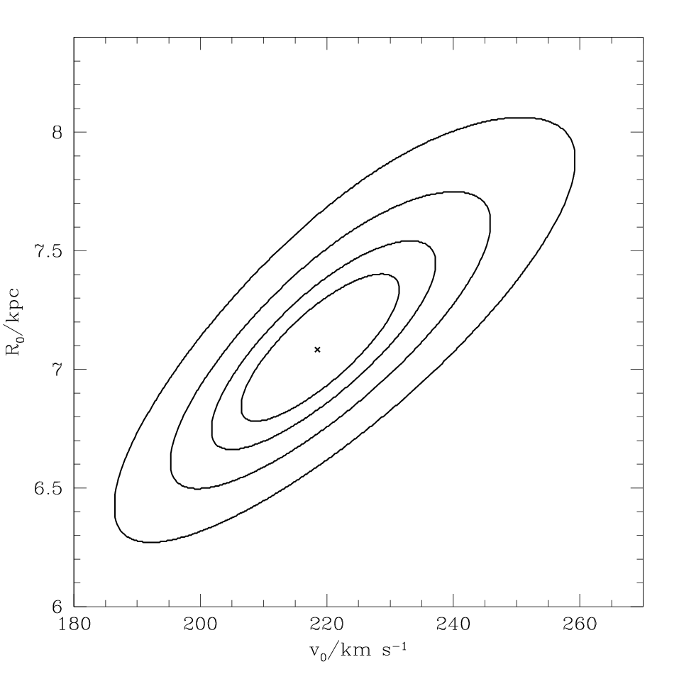
Table 1 gives the peak likelihoods of our models, as well as the best-fitting parameters and the corresponding uncertainties. The best-fitting value of $v_{0}$ varies in the range $(200-279)\,\mathrm{km\,s}^{-1}$, and that of $R_{0}$ between $6.7$ and $8.9\,\mathrm{kpc}$. As Fig. 2 illustrates, $v_{0}$ and $R_{0}$ are strongly correlated with the result that $v_{0}/R_{0}$ is confined to the relatively narrow range $29.9-31.6\,\mathrm{km\,s}^{-1}\,\,\mathrm{kpc}^{-1}$.

When $\mathbf{v_{\odot}}$ is a free parameter, the best-fitting values of $U_{\odot}$ and $W_{\odot}$ are close to the DB98 values, and essentially independent of the form of the rotation curve, whereas $V_{\odot}$ varies in the range $16.5-19.5\,\mathrm{km\,s}^{-1}$. Similarly, when $\mathbf{v_{\odot}}$ is fixed at the DB98 value and $\mathbf{v}_{\mathrm{SFR}}$ is a free parameter, only $v_{\phi,\rm SFR}$ takes a value that is far removed from that which one would naively expect – it moves in the range $-11.0$ to $-14.8\,\mathrm{km\,s}^{-1}$. Thus the data suggest either that the Sun is circulating significantly faster than the circular speed, or that the hmsfr have an appreciable rotational lag.

The fits are almost perfectly degenerate between $\mathbf{v_{\odot}}$ and $\mathbf{v}_{\mathrm{SFR}}$: they constrain only the difference between these velocities. However, we shall argue in Section 4 that significantly non-zero values of $\mathbf{v}_{\mathrm{SFR}}$ are physically implausible, so here we focus on what can be inferred about $\mathbf{v_{\odot}}$ given $\mathbf{v}_{\mathrm{SFR}}=0$. In view of the degeneracy between $\mathbf{v_{\odot}}$ and $\mathbf{v}_{\mathrm{SFR}}$ we do not report results obtained when both $\mathbf{v_{\odot}}$ and $\mathbf{v}_{\mathrm{SFR}}$ are varied.

When $\mathbf{v}_{\mathrm{SFR}}=0$, the peak likelihood is higher when $\mathbf{v_{\odot}}$ is fixed to the B09 value than when it is fixed to the DB98 value. To assess the significance of this increase in likelihood, we calculate the ratio of the evidences for the two models as described in Section 2.3.2

Thus regardless of the adopted rotation curve, the data strongly favour upward revision of $V_{\odot}$ from $5.2\,\mathrm{km\,s}^{-1}$ to $11\,\mathrm{km\,s}^{-1}$.

When $\mathbf{v_{\odot}}$ is a free parameter, the peak likelihood of the B09 model is surpassed at yet larger values of $V_{\odot}$. To determine whether the increase in likelihood that occurs when $\mathbf{v_{\odot}}$ is set free from the B09 value, we again calculate the relevant ratio of the evidences. Since the two models now differ in whether $\mathbf{v_{\odot}}$ is fixed or free, the priors on the components of $\mathbf{v_{\odot}}$ now become relevant (cf eq. 8). We have adopted $\Delta U_{\odot}=\Delta V_{\odot}=\Delta W_{\odot}=100\,\mathrm{km\,s}^{-1}$. With these values we have

Therefore under these assumptions the increase in likelihood attained on setting $\mathbf{v_{\odot}}$ free from the B09 value is not statistically significant. The ratio of evidences for the case when $\mathbf{v_{\odot}}$ is set to the DB98 value or is set free is

Therefore, even with a generous choice of $\Delta U_{\odot}$, etc., the data reject the possibility that the Sun has the DB98 value of $\mathbf{v_{\odot}}$. Reducing the widths $\Delta U_{\odot}$, etc., of the priors on $\mathbf{v_{\odot}}$ would strengthen the case against the DB98 value of $\mathbf{v_{\odot}}$.

The choice of $\Delta U_{\odot}\sim 100\,\mathrm{km\,s}^{-1}$ is reasonably generous, and it is sensible to ask what value of $\Delta U_{\odot}$, etc., would bring ${p(\mathrm{B09}|\mathrm{data})}/{p(\mathbf{v_{\odot}}\mathrm{\ free}|\mathrm{data})}$ down to unity. In the case where the GDII rotation curve is used, it would require a reduction to a value $\Delta U_{\odot}\sim 30\,\mathrm{km\,s}^{-1}$ – this is smaller than is reasonable given that the value for $V_{\odot}$ found when it is allowed to vary is already $\sim 15\,\mathrm{km\,s}^{-1}$ greater than the canonical DB98 value.

It is worth noting that the case for setting $\mathbf{v_{\odot}}$ free from either the DB98 value of the B09 value is weakest when the best-motivated rotation curve is adopted – the GDII curve.

The lowest values of both $v_{0}$ and $R_{0}$ are found for the models with the DB98 value of $\mathbf{v_{\odot}}$, and $\mathbf{v}_{\mathrm{SFR}}$ set to zero. Both $v_{0}$ and $R_{0}$ take larger values for models with the B09 value of $\mathbf{v_{\odot}}$, and larger still for models with either $\mathbf{v_{\odot}}$ or $\mathbf{v}_{\mathrm{SFR}}$ allowed to vary. The lowest values of $v_{0}$ and $R_{0}$ for the models in which the peculiar velocities are allowed to vary are $232\,\mathrm{km\,s}^{-1}$ and $7.7\,\mathrm{kpc}$ respectively.

Fig. 3 suggests a reason why the value of $\mathbf{v_{\odot}}$ or $\mathbf{v}_{\mathrm{SFR}}$ in the model has such a large impact on the best fitting values of $v_{0}$ and $R_{0}$. It shows the residual velocities of the objects after the expected velocity is subtracted (ignoring the uncertainty in parallax). The objects that provide the strongest indication that some change in peculiar motion is required (indicated by open squares) are all relatively close to the Sun. Consequently, changes in $R_{0}$ and $v_{0}$ have a relatively small “lever arm” with which to bring the model closer to the data, with rather large changes required in order to have any significant impact on the expected values of the observables for those objects. The introduction of a new peculiar velocity (either of the sources or the Sun) allows the model to compensate for the significant discrepancy between the velocity of these objects and those expected from the rotation curve, without producing a major effect on the best-fitting values of $R_{0}$ and $v_{0}$.

These results, and in particular the large variation in $v_{0}$ and $R_{0}$ depending on the other model parameters, makes it impossible to constrain tightly either $v_{0}$ or $R_{0}$ from these data – the smallest best-fitting values of these parameters are, respectively, 40 per cent and 33 per cent smaller than the largest best-fitting values. The choice of rotation curve has a significant impact, and we do not investigate all possible rotation curves. It is worth noting that our two most favoured models in Table 1 (according to Bayesian evidence, so somewhat dependent on our choice of priors) have best-fitting values of $v_{0}$ that differ by $30\,\mathrm{km\,s}^{-1}$ and of $R_{0}$ that differ by $1\,\mathrm{kpc}$ from one another (the models are those with B09 $\mathbf{v_{\odot}}$ $+$ GD rotation curve and free $\mathbf{v_{\odot}}$ $+$ power-law rotation curve, respectively).

However, for all but one of our models the best fitting $v_{0}/R_{0}$ lie in the narrow range $(29.8-31.5)\,\mathrm{km\,s}^{-1}\,\mathrm{kpc}^{-1}$, with typical uncertainties $\sim 1.5\,\mathrm{km\,s}^{-1}\,\mathrm{kpc}^{-1}$. This corresponds to best fitting $(v_{0}+V_{\odot})/R_{0}$ in the range $(30.9-32.5)\,\mathrm{km\,s}^{-1}\,\,\mathrm{kpc}^{-1}$ (again, depending on the model), with similar uncertainties. These values are slightly larger than the value of $(v_{0}+V_{\odot})/R_{0}=30.2\pm 0.2\,\mathrm{km\,s}^{-1}\,\mathrm{kpc}^{-1}$ found from the proper motion of Sgr A* (Reid & Brunthaler, 2004), but consistent to within (less than) twice the uncertainties on our values.

If we allow for a bias in the maser radial velocities with respect to the Sun by allowing the parameter $v_{\mathrm{m}}$ to take a non-zero value in equation (4), this does improve the fit. However we have seen that this is primarily due to a group of maser sources in the Perseus spiral arm, so the cause may be a large peculiar motion in that part of the Galaxy. Even if the bias in measured radial velocity is real, it does not affect the result: (i) that in different models these data are fit best by very different values of $v_{0}$ and $R_{0}$; (ii) that the DB98 $\mathbf{v_{\odot}}$ is rejected by these data, and (iii) that the B09 $\mathbf{v_{\odot}}$ is favoured over making $\mathbf{v_{\odot}}$ a free parameter.

Reid et al. (2009) focused on the idea that these data show that the hmsfrs are orbiting the Galaxy with a velocity that lags the circular speed by $-v_{\phi,\mathrm{SFR}}\sim 15\,\mathrm{km\,s}^{-1}$. Our analysis of similar models shows that the data are fit better by a slightly smaller offset of $(11-14.8)\,\mathrm{km\,s}^{-1}$ to the circular speed. We have also shown that an equivalent fit to the data can be obtained by instead increasing to $\sim 17\,\mathrm{km\,s}^{-1}$ the amount $V_{\odot}$ by which the Sun is assumed to circulate faster than the circular speed. In fact, the sources that provide the strongest statistical support for $v_{\phi,\mathrm{SFR}}\sim-15\,\mathrm{km\,s}^{-1}$ are found near the Sun (Fig. 3), so a change in $\mathbf{v_{\odot}}$ has a very similar effect to a change in $\mathbf{v}_{\mathrm{SFR}}$. More maser data at different Galactic azimuths could break this degeneracy, as well as reducing the correlation between the values of $v_{0}$ and $R_{0}$ seen in Fig. 2.

If the proposal of Reid et al. (2009) that $v_{\phi,\mathrm{SFR}}\simeq-15\,\mathrm{km\,s}^{-1}$ were correct, the hmsfrs would all have to be close to apocentre. Since the lifetime of an hmsfr is short compared to a typical epicycle period and spiral structure must play a significant role in their formation, it is not inherently implausible that the maser stars are all close to apocentre. However, two arguments make it unlikely that the maser stars are on orbits as eccentric as is implied by a $15\,\mathrm{km\,s}^{-1}$ offset from circular motion at apocentre.

First, non-axisymmetric structure in the Galaxy’s potential modulates the tangential velocity of gas by only $\sim 7\,\mathrm{km\,s}^{-1}$ (e.g. Binney & Merrifield, 1998, §9.2.3), so the hmsfrs would be moving with a peculiar velocity significantly higher than the gas from which they formed. Second, by GDII (equation 3.100), a quarter of an epicycle period later the $U$ velocities of these stars would be $(2\Omega/\kappa)15\,\mathrm{km\,s}^{-1}\simeq 22\,\mathrm{km\,s}^{-1}$, where $\Omega$ and $\kappa$ are the circular and radial frequencies at the star’s location. Hence the radial velocity dispersion of a population of such stars would be at least $\sim 22/\surd 2\simeq 15\,\mathrm{km\,s}^{-1}$. The velocity dispersion of stars observed locally increases with age on account of heating by irregularities in the Galaxy’s gravitational field (e.g. GDII §10.4.1) and the velocity dispersion of the bluer stars in the Hipparcos catalogue is $\sim 10\,\mathrm{km\,s}^{-1}$ (Aumer & Binney, 2009) rather than $15\,\mathrm{km\,s}^{-1}$. Thus the conjecture of Reid et al. (2009) not only requires the masing stars to be confined to apocentre but also requires them to have more eccentric orbits than the generality of young stars. Recognising this problem, Reid et al. suggested that the orbits of these stars became more circular early in their lives. However, any random scattering process spreads stars more widely in phase space and therefore increase the mean eccentricity of the masing stars. Only a dissipative process could increase the phase-space density of these stars by moving them to more circular orbits, and no such process is known.

If the B09 value of $V_{\odot}$ is correct, the lag to circular motion required to optimise the fit to the data is so small ($\sim 5\,\mathrm{km\,s}^{-1}$) that the above objections to the proposal that hmsfr systematically lag rotation become moot. However, the formalism of Bayesian inference says that when the B09 value of $V_{\odot}$ is accepted, there is no convincing evidence for a systematic lag of the hmsfr.

Throughout this paper we have proceeded under the assumption that the velocity of the LSR is the same thing as the circular velocity at $R_{0}$. It is worth noting that this is not necessarily the case. The LSR is defined to be the velocity of a closed orbit as it passes the current Solar position, which will only be a circular orbit if the Galactic potential is axisymmetric. Therefore the velocity of the LSR may be offset from the circular velocity curve. However (much like the possibility of a systematic lag of the hmsfr) we should note that if we accept the B09 value of $V_{\odot}$, there is no convincing evidence for this offset.

We conclude that these data provide a compelling case for revising $V_{\odot}$ upward. Our Bayesian analysis (equation 10) supports the revision upwards of $V_{\odot}$ to $11\,\mathrm{km\,s}^{-1}$ suggested by B09 on the basis of modelling predominantly old disc stars with relatively large random velocities. It should, however, be recognised that an even better fit to these data comes from somewhat larger upward revisions to $V_{\odot}\sim 16-20\,\mathrm{km\,s}^{-1}$.

We have reanalysed observations of hmsfrs reported in Reid et al. (2009) using a maximum-likelihood approach to exploit fully the data, in an effort to determine the values of $R_{0}$, the Galactocentric radius of the Sun, and $v_{0}$, the circular velocity of the LSR. We have found that the best-fitting values, considered separately, are strongly dependent on the Galaxy model used to interpret the data, but that the ratio $v_{0}/R_{0}$ is consistently found to lie in the range $29.8-31.5\,\mathrm{km\,s}^{-1}\,\,\mathrm{kpc}^{-1}$.

We have also used these data to explore the value of the Sun’s peculiar velocity $\mathbf{v_{\odot}}$, in light of the recent argument of B09 that the canonical DB98 value is incorrect. We find that these data support the conclusion that $V_{\odot}$ is significantly higher than the DB98 value. By a small but significant margin, the data prefer models with the B09 revision of $V_{\odot}$ to $\sim 11\,\mathrm{km\,s}^{-1}$ over models in which $\mathbf{v_{\odot}}$ is left as a free parameter (equation 10). The best-fitting models have $U_{\odot}$ and $W_{\odot}$ near to the DB98 values, and the even larger value of $V_{\odot}\sim 16-20\,\mathrm{km\,s}^{-1}$.

Reid et al. (2009) suggested that hmsfrs significantly lag circular rotation. We have investigated the possibility that the hmsfrs have a typical peculiar velocity $\mathbf{v}_{\mathrm{SFR}}$ and find that the models only constrain the velocity difference $\mathbf{v}_{\mathrm{SFR}}-\mathbf{v_{\odot}}$. We have argued that models in which the hmsfrs have large peculiar velocities in the opposite direction to Galactic rotation are neither needed nor plausible.

This work, in conjunction with B09, casts severe doubt on the accuracy of the widely used DB98 value for $V_{\odot}$. This must be a concern for anyone interested in the dynamics within the Milky Way because velocities are inevitably measured with respect to the Sun. Both observations of more masers and the development of a detailed dynamical model of the Galaxy’s spiral structure would contribute to establishing more securely what the true value of $V_{\odot}$ is.

We thank John Magorrian and the other members of the Oxford dynamics group for valuable discussions. PJM is supported by a grant from the Science and Technology Facilities Council.

After this paper was accepted for publication, Rygl et al. (2009) presented similar observations of maser sources. Incorporating these observations in our analysis does not materially affect our conclusions.

References

- Aumer & Binney (2009) Aumer M., Binney J. J., 2009, MNRAS, 397, 1286
- Binney & Merrifield (1998) Binney J., Merrifield M., 1998, Galactic astronomy. Princeton University Press
- Binney & Tremaine (2008) Binney J., Tremaine S., 2008, Galactic Dynamics: Second Edition. Princeton University Press
- Binney (2009) Binney J. J., 2009, MNRAS, accepted, arXiv:0910.1512 (B09)
- Chatterjee et al. (2002) Chatterjee P., Hernquist L., Loeb A., 2002, ApJ, 572, 371
- Dehnen & Binney (1998) Dehnen W., Binney J. J., 1998, MNRAS, 298, 387
- Gelman & Rubin (1992) Gelman A., Rubin D. B., 1992, Statistical Science, 7, 457
- Ghez et al. (2008) Ghez A. M., Salim S., Weinberg N. N., Lu J. R., Do T., Dunn J. K., Matthews K., Morris M. R., Yelda S., Becklin E. E., Kremenek T., Milosavljevic M., Naiman J., 2008, ApJ, 689, 1044
- Gillessen et al. (2009) Gillessen S., Eisenhauer F., Trippe S., Alexander T., Genzel R., Martins F., Ott T., 2009, ApJ, 692, 1075
- Heavens (2009) Heavens A., 2009, arXiv: 0906.0664
- Koposov et al. (2009) Koposov S. E., Rix H.-W., Hogg D. W., 2009, ApJ, submitted, (arXiv: 0907.1085)
- Metropolis et al. (1953) Metropolis N., Rosenbluth A. W., Rosenbluth M. N., Teller A. H., Teller E., 1953, Journal of Chemical Physics, 21, 1087–1092
- Reid (1993) Reid M. J., 1993, AnnRA&A, 31, 345
- Reid & Brunthaler (2004) Reid M. J., Brunthaler A., 2004, ApJ, 616, 872
- Reid et al. (2009) Reid M. J., Menten K. M., Zheng X. W., Brunthaler A., Moscadelli L., Xu Y., Zhang B., Sato M., Honma M., Hirota T., Hachisuka K., Choi Y. K., Moellenbrock G. A., Bartkiewicz A., 2009, ApJ, 700, 137
- Rygl et al. (2009) Rygl K. L. J., Brunthaler A., Reid M. J., Menten K. M., van Langevelde H. J., Xu Y., 2009, A&A, accepted (arXiv:0910.0150)