跳到论文正文
W Papers独立论文阅读器 arXiv:0907.4682 论文正文 计算阅读时间 · 0%
引用这篇论文根据当前论文元数据生成,正式投稿前建议核对。


License: arXiv.org perpetual non-exclusive license
arXiv:0907.4682v1 [hep-ph] 27 Jul 2009

RM3-TH/09-15

LAPTH-1337/09

On the radiative corrections to the neutral
Higgs boson masses in the NMSSM

G. Degrassia and P. Slavich𝒃,𝒄{}^{b,\,c}

a Dipartimento di Fisica, Università di Roma Tre and INFN, Sezione di Roma Tre
Via della Vasca Navale 84, I-00146 Rome, Italy

b LAPTH, 9, Chemin de Bellevue, F-74941 Annecy-le-Vieux, France

c LPTHE, 4, Place Jussieu, F-75252 Paris, France

We provide a full one-loop calculation of the self energies and tadpoles of the neutral Higgs bosons of the NMSSM. In addition, we compute the two-loop 𝒪⁡(αt​αs+αb​αs){\cal O}(\alpha_{t}\alpha_{s}+\alpha_{b}\alpha_{s}) corrections to the neutral Higgs boson masses in the effective potential approximation. With respect to earlier calculations, the newly-computed corrections can account for shifts of a few GeV in the light scalar and pseudoscalar masses, and they can also sizeably affect the mixing between singlet and MSSM-like Higgs scalars. Taking these corrections into account will be crucial for a meaningful comparison between the MSSM and NMSSM predictions for the Higgs sector.

00 0 e-mail:00 0 degrassi@fis.uniroma3.it00 0 slavich@lpthe.jussieu.fr

1 Introduction

The Next-to-Minimal Supersymmetric extension of the Standard Model, or NMSSM [1, 2, 3], provides an elegant solution to the μ\mu problem of the MSSM [4], i.e. the question of how to relate the higgsino mass parameter μ\mu appearing in the superpotential to the soft SUSY-breaking masses of the other supersymmetric particles. In the NMSSM the parameter μ\mu arises as the vacuum expectation value (vev) of the scalar component of an additional chiral superfield SS, singlet with respect to the SM gauge group and coupled to the MSSM Higgs superfields H1H_{1} and H2H_{2} through a superpotential term λ​S​H1​H2\lambda\,SH_{1}H_{2}\,. The scalar and pseudoscalar components of the singlet superfield mix with the MSSM Higgs fields of matching parity, while the fermion component (singlino) mixes with the MSSM higgsinos. The quartic Higgs scalar interaction controlled by the new coupling λ\lambda can bring the additional benefit of increasing the tree-level prediction for the mass of the lightest Higgs boson, which in the MSSM is bounded from above by the ZZ-boson mass, in contradiction with the lower bound from direct searches at LEP [5]. This increase allows for a smaller contribution to the Higgs mass from radiative corrections involving the top quark and its scalar partner, the stop, thus reducing the so-called little hierarchy problem of the MSSM, i.e. the need for the stop masses to be substantially larger than the weak scale. Another interesting feature of the NMSSM is the existence of scenarios in which a Higgs scalar with SM-like couplings to fermions and gauge bosons decays mainly into a pair of lighter scalars or pseudoscalars, requiring a refinement of the strategies for Higgs searches at the Tevatron and at the LHC [6, 7]. A SM-like Higgs scalar decaying into a pair of pseudoscalars which are in turn too light to decay into bb quarks might even have already been produced at the LEP, and escaped detection because of its non-standard decay chain [8].

Due to the crucial role of radiative corrections in pushing the prediction for the lightest Higgs boson mass above the LEP bound, an impressive theoretical effort has been devoted in the past two decades to the precise determination of the Higgs sector of the MSSM [9]. After the early realization [10] of the importance of the one-loop 𝒪⁡(αt){\cal O}(\alpha_{t}) corrections11 1 We define αt,b=ht,b2/(4​π)\alpha_{t,b}=h_{t,b}^{2}/(4\pi), where hth_{t} and hbh_{b} are the superpotential top and bottom couplings, respectively. Here and in the following we denote for brevity as 𝒪⁡(αt){\cal O}(\alpha_{t}) the one-loop corrections to the Higgs masses that are in fact proportional to αt​mt2\alpha_{t}m_{t}^{2}, i.e. αt2​v22\alpha_{t}^{2}v_{2}^{2}. Similar abuses of notation affect the other one- and two-loop corrections. involving top and stop, full one-loop computations of the MSSM Higgs masses have been provided [11, 12], leading logarithmic effects at two loops have been included via appropriate renormalization group equations [13], and genuine two-loop corrections of 𝒪⁡(αt​αs){\cal O}(\alpha_{t}\alpha_{s}) [14, 15, 16, 17, 18], 𝒪⁡(αt2){\cal O}(\alpha_{t}^{2}) [14, 17, 19], 𝒪⁡(αb​αs){\cal O}(\alpha_{b}\alpha_{s}) [20, 21] and 𝒪⁡(αt​αb+αb2){\cal O}(\alpha_{t}\alpha_{b}+\alpha_{b}^{2}) [22] have been evaluated in the limit of zero external momentum. All of these corrections have been implemented in public computer codes [23, 24] for the calculation of the MSSM mass spectrum. More recently, a nearly complete two-loop calculation of the MSSM Higgs masses, including electroweak effects and part of the external momentum dependence, has been performed [25], and even the leading three-loop effects have been computed [26]. Finally, a vast literature [27] is available on the dominant one- and two-loop corrections to the MSSM Higgs masses in the presence of CP-violating phases in the soft SUSY-breaking parameters.

In comparison with the case of the MSSM, the computation of the radiative corrections to the Higgs masses in the NMSSM is not quite as advanced. The one-loop contributions from diagrams involving top/stop and bottom/sbottom loops have been computed [28] only in the effective potential approximation, i.e. neglecting the external momentum in the self energies. For what concerns the one-loop contributions from diagrams involving chargino, neutralino or scalar loops (the contributions arising from gauge-boson loops are the same as in the MSSM) only the leading logarithmic terms have been computed [29]. Similarly, among the two-loop contributions only the leading-logarithmic 𝒪⁡(αt​αs){\cal O}(\alpha_{t}\alpha_{s}) and 𝒪⁡(αt2){\cal O}(\alpha_{t}^{2}) terms – borrowed from the MSSM results under the simplifying assumption of fully degenerate SUSY masses – have been taken into account so far. All of these corrections have been implemented in a public computer code, NMHDECAY [30], which computes masses, couplings and decay widths of the NMSSM Higgs bosons.

It is clear that, for a proper comparison between the MSSM and NMSSM predictions and for a precise characterization of the scenarios of refs. [6, 8], it would be desirable to compute the masses and mixings in the NMSSM Higgs sector with an accuracy comparable to that of the calculations implemented in the public MSSM codes of ref. [24]. In this paper we take a few steps in this direction. First of all, we provide explicit formulae for the one-loop corrections to the mass matrices of the neutral CP-even and CP-odd Higgs bosons. In addition, we compute the two-loop 𝒪⁡(αt​αs+αb​αs){\cal O}(\alpha_{t}\alpha_{s}+\alpha_{b}\alpha_{s}) corrections in the approximation of zero external momentum, adapting to the NMSSM case the techniques (and, in part, the results) developed for the MSSM in refs. [18, 19, 22, 31]. To fully match the accuracy of the MSSM codes it would also be necessary to include the two-loop 𝒪⁡(αt2+αt​αb+αb2){\cal O}(\alpha_{t}^{2}+\alpha_{t}\alpha_{b}+\alpha_{b}^{2}) corrections. These corrections, however, cannot be straightforwardly adapted from the MSSM case and require a dedicated calculation. We leave that, as well as a detailed re-analysis of the NMSSM parameter space taking into account the improvements in the Higgs mass calculation, to a future publication.

The paper is organized as follows. After this introduction, in section 2 we describe the Higgs sector of the NMSSM. In section 3 we describe the diagrammatic calculation of the one-loop corrections to the CP-odd and CP-even Higgs mass matrices. In section 4 we describe the effective potential calculation of the two-loop 𝒪⁡(αt​αs+αb​αs){\cal O}(\alpha_{t}\alpha_{s}+\alpha_{b}\alpha_{s}) corrections. In section 5 we show numerical results for some representative scenarios. In section 6 we conclude. Finally, appendix A contains the definitions of the couplings that enter the calculation of the one-loop radiative corrections; appendix B provides the explicit expressions for the one-loop self energies and tadpoles that appear in the computation of the Higgs boson masses; appendix C contains the formulae for the two-loop corrections in terms of derivatives of the effective potential; appendix D contains the definitions of the functions entering the two-loop results.

2 The Higgs sector of the NMSSM

In the SLHA conventions [32, 33] the NMSSM superpotential for the Higgs superfields H1,H2,SH_{1},\,H_{2},\,S and the quark and lepton superfields Q,Uc,Dc,L,EcQ,\,U^{c}\!\!,\,D^{c}\!,\,L\,,\,E^{c} reads

W=he​H1​L​Ec+hd​H1​Q​Dc+hu​Q​H2​Uc−λ​S​H1​H2+κ3​S3,W~=~h_{e}\,H_{1}LE^{c}+h_{d}\,H_{1}QD^{c}+h_{u}\,QH_{2}U^{c}-\lambda\,SH_{1}H_{2}+\frac{\kappa}{3}\,S^{3}~, (1)

where we neglect colour and generation indices. The S​U​(2)SU(2)-doublet superfields are contracted by the antisymmetric tensor ϵa​b\epsilon_{ab}, with ϵ12=1\epsilon_{12}=1. The corresponding terms in the soft SUSY-breaking scalar potential are

Vsoft\displaystyle V_{\rm soft}\!\! =\displaystyle= mH12​H1†​H1+mH22​H2†​H2+mS2​S∗​S+mQ2​Q†​Q+mL2​L†​L+mU2​u~R∗​u~R+mD2​d~R∗​d~R+mE2​e~R∗​e~R\displaystyle\!\!m_{H_{1}}^{2}H_{1}^{\dagger}H_{1}+m_{H_{2}}^{2}H_{2}^{\dagger}H_{2}+m_{S}^{2}\,S^{*}S+m_{Q}^{2}\,Q^{\dagger}Q+m_{L}^{2}\,L^{\dagger}L+m_{U}^{2}\,\tilde{u}_{R}^{*}\tilde{u}_{R}+m_{D}^{2}\,\tilde{d}_{R}^{*}\tilde{d}_{R}+m_{E}^{2}\,\tilde{e}_{R}^{*}\tilde{e}_{R} (2)
+\displaystyle+ (heAeH1Le~R∗+hdAdH1Qd~R∗+huAuQH2u~R∗−λAλSH1H2+κ3AκS3+h.c.),\displaystyle\!\!\left(h_{e}\,A_{e}\,H_{1}L\,{\tilde{e}_{R}}^{*}+h_{d}\,A_{d}\,H_{1}Q\,\tilde{d}_{R}^{*}+h_{u}\,A_{u}\,QH_{2}\,\tilde{u}_{R}^{*}-\lambda\,A_{\lambda}\,SH_{1}H_{2}+\frac{\kappa}{3}\,A_{\kappa}\,S^{3}~+~{\rm h.c.}\right),

where for the scalar components of the quark and lepton superfields we define u~R=Uc∗\tilde{u}_{R}=U^{c\,*}, d~R=Dc∗\tilde{d}_{R}=D^{c\,*}, e~R=Ec∗\tilde{e}_{R}=E^{c\,*}, Q=(u~L,d~L)TQ=(\tilde{u}_{L},\tilde{d}_{L})^{T} and L=(ν~L,e~L)TL=(\tilde{\nu}_{L},\tilde{e}_{L})^{T}. For simplicity, we take the soft SUSY-breaking trilinear couplings (as well as the gaugino masses) to be all real, and we neglect inter-generational squark and slepton mixing.

The neutral components of the Higgs fields can be decomposed into their vevs plus their CP-even and CP-odd fluctuations as

Hi0=vi+12​(Si+i​Pi)​(i=1,2),S=vs+12​(S3+i​P3).H_{i}^{0}~=~v_{i}+\frac{1}{\sqrt{2}}\,(S_{i}+iP_{i})~~(i=1,2)~,~~~~~~~~~S~=~v_{s}+\frac{1}{\sqrt{2}}\,(S_{3}+iP_{3})~. (3)

Using the minimization conditions of the tree-level scalar potential V0V_{0} to replace the soft SUSY-breaking Higgs masses mH12,mH22m_{H_{1}}^{2},\,m_{H_{2}}^{2} and mS2m_{S}^{2} with combinations of the Higgs vevs and the trilinear couplings, the tree-level mass matrix for the CP-even fields, (ℳS2)tree\left({\cal M}^{2}_{S}\right)^{\rm tree}, reads

(g¯2​v12+λ​vs​v2v1​AΣ(2​λ2−g¯2)​v1​v2−λ​vs​AΣ2​λ2​v1​vs−λ​v2​(AΣ+κ​vs)(2​λ2−g¯2)​v1​v2−λ​vs​AΣg¯2​v22+λ​vs​v1v2​AΣ2​λ2​v2​vs−λ​v1​(AΣ+κ​vs)2​λ2​v1​vs−λ​v2​(AΣ+κ​vs)2​λ2​v2​vs−λ​v1​(AΣ+κ​vs)λ​Aλ​v1​v2vs+κ​vs​(Aκ+4​κ​vs)),\left(\begin{array}[]{ccc}\bar{g}^{2}v_{1}^{2}+\lambda\,v_{s}\,\frac{v_{2}}{v_{1}}\,A_{\Sigma}&(2\lambda^{2}-\bar{g}^{2})v_{1}v_{2}-\lambda\,v_{s}\,A_{\Sigma}&2\lambda^{2}\,v_{1}\,v_{s}-\lambda\,v_{2}\,(A_{\Sigma}+\kappa\,v_{s})\\ (2\lambda^{2}-\bar{g}^{2})v_{1}v_{2}-\lambda\,v_{s}\,A_{\Sigma}&\bar{g}^{2}v_{2}^{2}+\lambda\,v_{s}\,\frac{v_{1}}{v_{2}}\,A_{\Sigma}&2\lambda^{2}\,v_{2}\,v_{s}-\lambda\,v_{1}\,(A_{\Sigma}+\kappa\,v_{s})\\ 2\lambda^{2}\,v_{1}\,v_{s}-\lambda\,v_{2}\,(A_{\Sigma}+\kappa\,v_{s})&2\lambda^{2}\,v_{2}\,v_{s}-\lambda\,v_{1}\,(A_{\Sigma}+\kappa\,v_{s})&\lambda\,A_{\lambda}\,\frac{v_{1}v_{2}}{v_{s}}+\kappa v_{s}\,(A_{\kappa}+4\,\kappa\,v_{s})\end{array}\right)~, (4)

where for brevity we define AΣ=Aλ+κ​vsA_{\Sigma}=A_{\lambda}+\kappa\,v_{s} and g¯2=(g2+g′ 2)/2\bar{g}^{2}=(g^{2}+g^{\prime\,2})/2, g\,g and g′g^{\prime} being the electroweak gauge couplings. The CP-even mass matrix is diagonalized by an orthogonal matrix RSR^{\scriptscriptstyle S}, such that

hi=Ri​jS​Sj,h_{i}=R^{\scriptscriptstyle S}_{ij}\,S_{j}~, (5)

where hih_{i}, with i=1,2,3i=1,2,3, are the CP-even mass eigenstates ordered by increasing mass. The tree-level mass matrix for the CP-odd fields, (ℳP2)tree\left({\cal M}^{2}_{P}\right)^{\rm tree}, reads

(λ​vs​v2v1​AΣλ​vs​AΣλ​v2​(AΣ−3​κ​vs)λ​vs​AΣλ​vs​v1v2​AΣλ​v1​(AΣ−3​κ​vs)λ​v2​(AΣ−3​κ​vs)λ​v1​(AΣ−3​κ​vs)4​λ​κ​v1​v2+λ​Aλ​v1​v2vs−3​κ​Aκ​vs).\left(\begin{array}[]{ccc}\lambda\,v_{s}\,\frac{v_{2}}{v_{1}}\,A_{\Sigma}&\lambda\,v_{s}\,A_{\Sigma}&\lambda\,v_{2}\,(A_{\Sigma}-3\,\kappa\,v_{s})\\ \lambda\,v_{s}\,A_{\Sigma}&\lambda\,v_{s}\,\frac{v_{1}}{v_{2}}\,A_{\Sigma}&\lambda\,v_{1}\,(A_{\Sigma}-3\,\kappa\,v_{s})\\ \lambda\,v_{2}\,(A_{\Sigma}-3\,\kappa\,v_{s})&\lambda\,v_{1}\,(A_{\Sigma}-3\,\kappa\,v_{s})&4\,\lambda\,\kappa\,v_{1}\,v_{2}+\lambda\,A_{\lambda}\,\frac{v_{1}v_{2}}{v_{s}}-3\,\kappa\,A_{\kappa}\,v_{s}\end{array}\right)~. (6)

The CP-odd mass matrix is in turn diagonalized by an orthogonal matrix RPR^{\scriptscriptstyle P}, such that

ai=Ri​jP​Pj,a_{i}=R^{\scriptscriptstyle P}_{ij}\,P_{j}~, (7)

where aia_{i} stands for (G0,A1,A2)(G^{0},A_{1},A_{2}). Here, G0G^{0} is the neutral pseudo-Goldstone boson, while A1A_{1} and A2A_{2} are the other CP-odd mass eigenstates, ordered by increasing mass. A commonly adopted procedure (see, e.g., the first paper in ref. [2]) consists in expressing P1P_{1} and P2P_{2} in terms of G0G^{0} and the orthogonal combination A0A^{0}, then defining a new ×22\!\times\!2 orthogonal matrix, RP′R^{{\scriptscriptstyle P}\,\prime}, which rotates (A0,P3)(A^{0},P_{3}) into (A1,A2)(A_{1},A_{2}). However, we will follow the SLHA prescription and refrain from this simplification.

In the neutralino sector, the singlino s~\tilde{s} mixes with the neutral components of the MSSM higgsinos h~10\tilde{h}_{1}^{0} and h~20\tilde{h}_{2}^{0}, which in turn mix with the neutral gauginos b~\tilde{b} and w~0\tilde{w}^{0}. In the formalism of two-component spinors, the Lagrangian contains the mass terms

−12​(−i​b~−i​w~0​h~10​h~20​s~)​(M10−g′v1/2g′​v2/200M2g​v1/2−gv2/20−g′v1/2g′​v2/20−λ​vs−λ​v2g​v1/2−gv2/2−λ​vs0−λ​v100−λ​v2−λ​v12​κ​vs)​(−i​b~−i​w~0h~10h~20s~),-\frac{1}{2}\,\left(-i\tilde{b}~-i\tilde{w}^{0}~~\tilde{h}_{1}^{0}~~\tilde{h}_{2}^{0}~~\tilde{s}\right)\,\left(\begin{array}[]{ccccc}M_{1}&0&-g^{\prime}\,v_{1}/\sqrt{2}&g^{\prime}\,v_{2}/\sqrt{2}&0\\ 0&M_{2}&g\,v_{1}/\sqrt{2}&-g\,v_{2}/\sqrt{2}&0\\ -g^{\prime}\,v_{1}/\sqrt{2}&g^{\prime}\,v_{2}/\sqrt{2}&0&-\lambda\,v_{s}&-\lambda\,v_{2}\\ g\,v_{1}/\sqrt{2}&-g\,v_{2}/\sqrt{2}&-\lambda\,v_{s}&0&-\lambda\,v_{1}\\ 0&0&-\lambda\,v_{2}&-\lambda\,v_{1}&2\,\kappa\,v_{s}\end{array}\right)\,\left(\begin{array}[]{c}-i\tilde{b}\\ -i\tilde{w}^{0}\\ \tilde{h}_{1}^{0}\\ \tilde{h}_{2}^{0}\\ \tilde{s}\end{array}\right)~, (8)

where M1M_{1} and M2M_{2} are the soft SUSY-breaking gaugino masses. The neutralino mass matrix is diagonalized by a unitary matrix NN, such that

χi0=Ni​j​ψj0,\chi^{0}_{i}=N_{ij}\,\psi^{0}_{j}~, (9)

where ψ0\psi^{0} stands for (−i​b~,−i​w~0,h~10,h~20,s~)(-i\tilde{b},\,-i\tilde{w}^{0},\,\tilde{h}_{1}^{0},\,\tilde{h}_{2}^{0},\,\tilde{s}) and χi0\chi^{0}_{i} are the neutralino mass eigenstates ordered by increasing mass. Under our simplifying assumptions all the entries of the neutralino mass matrix in eq. (8) can be taken as real. In this case NN becomes a real matrix, as long as the neutralino mass terms are allowed to take on negative signs.

Finally, the charged-Higgs and chargino sectors of the NMSSM are not directly affected by the presence of the singlet superfield. The expressions for the corresponding mass matrices are the same as in the MSSM, once we identify

tan⁡β≡v2v1,μ≡λ​vs,Bμ≡λ​vs​AΣ−λ2​v1​v2,\tan\beta~\equiv~\frac{v_{2}}{v_{1}}\,,~~~~~~~\mu~\equiv~\lambda\,v_{s}\,,~~~~~~~B_{\mu}~\equiv~\lambda\,v_{s}\,A_{\Sigma}-\lambda^{2}\,v_{1}v_{2}~, (10)

where μ\mu is the usual Higgs mass term in the MSSM superpotential and BμB_{\mu} is the corresponding term in the soft SUSY-breaking scalar potential. In particular, the chargino mass matrix is as in eq. (22) of ref. [32], and the charged-Higgs mass is

mH+2=Bμsin⁡β​cos⁡β+MW2.m_{H^{+}}^{2}~=~\frac{B_{\mu}}{\sin\beta\cos\beta}~+~M_{W}^{2}~. (11)

From eqs. (4), (6) and (8) it can be seen that, when λ≪1\lambda\ll 1, the singlet and the singlino decouple from the Higgs and higgsino sectors of the MSSM, respectively. Since the experimental lower bounds on the chargino masses require μ\mu to be (at least) of the order of 100 GeV, eq. (10) implies that, in this limit, vs≫(v1,v2)v_{s}\gg(v_{1},v_{2})\,, so that Bμ≈λ​κ​vs2B_{\mu}\approx\lambda\,\kappa\,v_{s}^{2} is driven to rather large values – leading in turn to the so-called decoupling limit of the MSSM – unless κ≪1\kappa\ll 1 as well.

3 One-loop corrections to the Higgs mass matrices

In this section we describe the calculation of the one-loop corrections to the neutral Higgs boson masses in the NMSSM. We follow closely the approach22 2 There are however a few differences between our conventions and those of ref. [12]: we normalize the Higgs vevs in such a way that (v12+v22)≈(174CLOSE(v_{1}^{2}+v_{2}^{2})\approx(174 GeVOPEN)2)^{2}, and our convention for the sign of the term λ​S​H1​H2\lambda\,SH_{1}H_{2} in the superpotential corresponds to the opposite sign of μ\mu w.r.t. ref. [12]. of the MSSM calculation of ref. [12], which is the one implemented in most public computer codes [24] that compute the mass spectrum of the MSSM.

Including the one-loop corrections in the DR¯\overline{\rm DR} renormalization scheme, and using the minimization conditions of the scalar potential to replace the soft SUSY-breaking Higgs masses with combinations of the other parameters, the 3×33\times 3 mass matrices for the CP-even and CP-odd fields read

(ℳS2)i​j1​l​o​o​p\displaystyle\left({\cal M}^{2}_{S}\right)^{\rm 1loop}_{ij} =\displaystyle= (ℳS2)i​jtree+12​δi​jvi​Ti−Πsi​sj​(p2)\displaystyle\left({\cal M}^{2}_{S}\right)^{\rm tree}_{ij}~+~\frac{1}{\sqrt{2}}\,\frac{\delta_{ij}}{v_{i}}\,T_{i}~-~\Pi_{s_{i}s_{j}}(p^{2}) (12)
(ℳP2)i​j1​l​o​o​p\displaystyle\left({\cal M}^{2}_{P}\right)^{\rm 1loop}_{ij} =\displaystyle= (ℳP2)i​jtree+12​δi​jvi​Ti−Πpi​pj​(p2)\displaystyle\left({\cal M}^{2}_{P}\right)^{\rm tree}_{ij}~+~\frac{1}{\sqrt{2}}\,\frac{\delta_{ij}}{v_{i}}\,T_{i}~-~\Pi_{p_{i}p_{j}}(p^{2}) (13)

where: the tree-level mass matrices (ℳS2)tree\left({\cal M}^{2}_{S}\right)^{\rm tree} and (ℳP2)tree\left({\cal M}^{2}_{P}\right)^{\rm tree}\! are given in eqs. (4) and (6), respectively, and they are expressed in terms of DR¯\overline{\rm DR}-renormalized parameters; viv_{i} stands for (v1,v2,vs)(v_{1},v_{2},v_{s}); TiT_{i} is the finite part of the one-loop tadpole diagram for the scalar SiS_{i}; Πsi​sj​(p2)\Pi_{s_{i}s_{j}}(p^{2}) and Πpi​pj​(p2)\Pi_{p_{i}p_{j}}(p^{2}) are the finite parts of the one-loop self energies for scalars and pseudoscalars, respectively; p2p^{2} is the external momentum flowing in the self energy. The explicit formulae for the scalar and pseudoscalar self energies and for the scalar tadpoles are collected in appendix B. We checked that, in the limit in which λ→0\lambda\rightarrow 0 while μ≡λ​vs\mu\equiv\lambda\,v_{s} is constant, our results for the ×22\!\times\!2 upper-left submatrix of Πsi​sj\Pi_{s_{i}s_{j}} and for the tadpoles T1T_{1} and T2T_{2} coincide with the MSSM results of ref. [12], as does the pseudoscalar self energy ΠA​A\Pi_{AA} that we can obtain by rotating the ×22\!\times\!2 upper-left submatrix of Πpi​pj\Pi_{p_{i}p_{j}} by an angle β\beta.

The radiatively corrected squared mass of the nn-th scalar or (physical) pseudoscalar can be obtained by solving iteratively for the nn-th eigenvalue of the corresponding mass matrix evaluated at an external momentum p2p^{2} equal to the mass eigenvalue itself (we remark that this procedure includes in the results for the masses also contributions that are formally of higher order in the perturbative expansion). On the other hand, there is a well-known ambiguity in the definition of the radiatively corrected mixing matrices RSR^{\scriptscriptstyle S} and RPR^{\scriptscriptstyle P}, because the rotations that diagonalize the radiatively corrected mass matrices depend on the choice of external momentum in the self energies. This ambiguity reflects the fact that the mixing matrices themselves are not physical observables. In our analysis we will define the radiatively corrected mixing matrix as the one that diagonalizes the mass matrix at p2=0p^{2}=0. This corresponds to the result obtained in the effective potential approximation.

The tree-level mass matrices in eqs. (12) and (13) depend on the combination of gauge couplings g¯2\bar{g}^{2}, on the NMSSM superpotential couplings λ\lambda and κ\kappa and on the three vevs v1,v2v_{1},v_{2} and vsv_{s}. As long as no experimental information on the parameters of the NMSSM Higgs sector (nor on the validity of the NMSSM itself) is available, λ,κ,vs\lambda,\,\kappa,\,v_{s} and the ratio of vevs tan⁡β\tan\beta can be considered directly as DR¯\overline{\rm DR}-renormalized inputs at some reference scale Q0Q_{0}. On the other hand, the DR¯\overline{\rm DR} values of v2≡v12+v22v^{2}\equiv v_{1}^{2}+v_{2}^{2}, gg and g′g^{\prime} can be extracted from the experimentally known SM observables. For example, starting from the muon decay constant GμG_{\mu} and the gauge-boson pole masses, we can make use of the relations

v−2=2​2​Gμ​(1−ΠW​WT​(0)MW2−δVB),v^{-2}~=~2\sqrt{2}\,G_{\mu}\,\left(1-\frac{\Pi^{T}_{WW}(0)}{M_{W}^{2}}-\delta_{\rm VB}\right)~, (14)
g¯2=v−2​MZ2​(1+ΠZ​ZT​(MZ2)MZ2),g2=2​v−2​MW2​(1+ΠW​WT​(MW2)MW2).\bar{g}^{2}~=~v^{-2}\,M_{Z}^{2}\,\left(1+\frac{\Pi^{T}_{ZZ}(M_{Z}^{2})}{M_{Z}^{2}}\right)~,~~~~~~g^{2}~=~2\,v^{-2}\,M_{W}^{2}\,\left(1+\frac{\Pi^{T}_{WW}(M_{W}^{2})}{M_{W}^{2}}\right)~. (15)

In eqs. (14) and (15), ΠV​VT​(p2)​(V=Z,W)\Pi^{T}_{VV}(p^{2})~~(V=Z,W) denotes the finite and transverse part of the self energy of the vector bosons, while δVB\delta_{\rm VB} denotes the sum of vertex, box and wave-function-renormalization corrections to the muon decay amplitude. The explicit formulae for the vector-boson self energies are collected in appendix B. The SM contribution to δVB\delta_{\rm VB} was computed long ago [34], and the SUSY contribution can be obtained from the MSSM results given in eqs. (C.13)–(C.22) of ref. [12], by simply extending the sum over the neutralinos to the five mass eigenstates of the NMSSM.

4 Two-loop corrections in the effective potential approach

We now discuss the computation of the two-loop corrections to the NMSSM Higgs mass matrices in the effective potential approach. The effective potential for the neutral Higgs sector can be decomposed as Veff=V0+Δ​VV_{\rm eff}=V_{0}+\Delta V, where Δ​V\Delta V contains the radiative corrections. The 3×33\times 3 mass matrices for the CP-even and CP-odd fields can be decomposed as

(ℳS2)i​jeff=(ℳS2)i​jtree+(Δ​ℳS2)i​j,(ℳP2)i​jeff=(ℳP2)i​jtree+(Δ​ℳP2)i​j,\left({\cal M}^{2}_{S}\right)^{\rm eff}_{ij}~=~\left({\cal M}^{2}_{S}\right)^{\rm tree}_{ij}+\left(\Delta{\cal M}^{2}_{S}\right)_{ij}~,~~~~~~~~~~\left({\cal M}^{2}_{P}\right)^{\rm eff}_{ij}~=~\left({\cal M}^{2}_{P}\right)^{\rm tree}_{ij}+\left(\Delta{\cal M}^{2}_{P}\right)_{ij}~, (16)

and the radiative corrections to the mass matrices are

(Δ​ℳS2)i​j\displaystyle\left(\Delta{\cal M}^{2}_{S}\right)_{ij} =\displaystyle= −12​δi​jvi​∂Δ​V∂Si|min+∂2Δ​V∂Si​∂Sj|min,\displaystyle-\frac{1}{\sqrt{2}}\,\frac{\delta_{ij}}{v_{i}}\left.\frac{\partial\Delta V}{\partial S_{i}}\right|_{\rm min}~+~\left.\frac{\partial^{2}\Delta V}{\partial S_{i}\partial S_{j}}\right|_{\rm min}~, (17)
(Δ​ℳP2)i​j\displaystyle\left(\Delta{\cal M}^{2}_{P}\right)_{ij} =\displaystyle= −12​δi​jvi​∂Δ​V∂Si|min+∂2Δ​V∂Pi​∂Pj|min,\displaystyle-\frac{1}{\sqrt{2}}\,\frac{\delta_{ij}}{v_{i}}\left.\frac{\partial\Delta V}{\partial S_{i}}\right|_{\rm min}~+~\left.\frac{\partial^{2}\Delta V}{\partial P_{i}\partial P_{j}}\right|_{\rm min}~, (18)

where viv_{i} stands for (v1,v2,vs)(v_{1},v_{2},v_{s}), and the derivatives of the correction Δ​V\Delta V are computed at the minimum of VeffV_{\rm eff}. The comparison between eqs. (17) and (18) and eqs. (12) and (13) highlights the correspondence between tadpoles, self energies and derivatives of the effective potential. In the calculation of the MSSM Higgs boson masses it is customary to reorganize the corrections in such a way that (ℳS2)tree\left({\cal M}^{2}_{S}\right)^{\rm tree} is expressed in terms of the non-zero eigenvalue of (ℳP2)eff\left({\cal M}^{2}_{P}\right)^{\rm eff}, which in the effective potential approximation corresponds to the physical AA-boson mass. In the case of the NMSSM this reorganization is not as practical, because there are two non-zero eigenvalues of (ℳP2)eff\left({\cal M}^{2}_{P}\right)^{\rm eff}. While it is possible to absorb some of the radiative corrections in an “effective” trilinear coupling A~λ\widetilde{A}_{\lambda}, this parameter does not allow for a direct physical interpretation. Therefore, we refrain from this manipulation as well and leave eq. (17) as it stands. Throughout the calculation we assume that all the parameters entering both the tree-level and one-loop parts of the mass matrices are renormalized in the DR¯\overline{\rm DR} scheme at a renormalization scale that we denote by QQ.

The 𝒪⁡(αs){\cal O}(\alpha_{s}) contribution to Δ​V\Delta V from two-loop diagrams involving top, stop, gluon and gluino has been computed e.g. in refs. [16, 18]. It is the same for the MSSM and for the NMSSM, and we give it for completeness in appendix C. The corresponding 𝒪⁡(αt​αs){\cal O}(\alpha_{t}\alpha_{s}) corrections to the mass matrices in eqs. (17) and (18) can in turn be computed by exploiting the Higgs-field dependence of the parameters appearing in Δ​V\Delta V. As detailed in ref. [18], if we neglect D-term contributions controlled by the electroweak gauge couplings the parameters in the top/top sector depend on the neutral Higgs fields only through two combinations:

X≡|X|ei​φ=htH20,X~≡|X~|ei​φ~=ht(AtH20−λS∗H10∗).X~\equiv~|X|\,e^{i\varphi}~=~h_{t}\,H_{2}^{0}~,~~~~~\widetilde{X}~\equiv~|\widetilde{X}|\,e^{i\tilde{\varphi}}~=~h_{t}\,\left(A_{t}\,H_{2}^{0}-\lambda\,S^{*}\,H_{1}^{0\,*}\right)\,. (19)

The top/stop 𝒪⁡(αs){\cal O}(\alpha_{s}) contribution to Δ​V\Delta V can be expressed in terms of five field-dependent parameters, which can be chosen as follows. The squared top and stop masses

mt2=|X|2,mt~1,22=12​[(mQ2+mU2+2​|X|2)±(mQ2−mU2)2+4​|X~|2],m_{t}^{2}=|X|^{2}~,~~~~~~~m^{2}_{\tilde{t}_{1,2}}=\frac{1}{2}\left[(m_{Q}^{2}+m_{U}^{2}+2\,|X|^{2}\,)\pm\sqrt{(m_{Q}^{2}-m_{U}^{2})^{2}+4\,|\widetilde{X}|^{2}}\,\right]~, (20)

a mixing angle θ¯t~\bar{\theta}_{\tilde{t}}, with 0≤θ¯t~≤π/20\leq\bar{\theta}_{\tilde{t}}\leq\pi/2, which diagonalizes the stop mass matrix after the stop fields have been redefined to make it real and symmetric

sin⁡2​θ¯t~=2​|X~|mt~12−mt~22,\sin 2\,\bar{\theta}_{\tilde{t}}=\frac{2\,|\widetilde{X}|}{m_{\tilde{t}_{1}}^{2}-m_{\tilde{t}_{2}}^{2}}~, (21)

and a combination of the phases of XX and X~\widetilde{X} that we can choose as

cos⁡(φ−φ~)=Re⁡(X~)​Re​(X)+Im⁡(X~)​Im​(X)|X~|​|X|.\cos\,(\varphi-\tilde{\varphi})=\frac{{\rm Re}(\widetilde{X})\,{\rm Re}(X)+{\rm Im}(\widetilde{X})\,{\rm Im}(X)}{|\widetilde{X}|\,|X|}\,. (22)

A sixth parameter, the gluino mass mg~m_{\tilde{g}}, does not depend on the Higgs background. In the following we will also refer to θt\theta_{t}, with −π/2<θt<π/2-\pi/2<\theta_{t}<\pi/2, i.e. the usual field-independent mixing angle that diagonalizes the stop mass matrix at the minimum of the scalar potential.

With a lengthy but straightforward application of the chain rule for the derivatives of the effective potential, the corrections to the Higgs mass matrices in eqs. (17) and (18) can be expressed as 33 3 The differences with respect to eqs. (25)–(30) of ref. [18] have multiple origins: we do not absorb part of the corrections in the tree-level mass matrices; we adopt the opposite convention for the sign of μ\mu; we take directly the derivatives of the renormalized effective potential as in refs. [22, 31], removing the need for the counterterm-induced shifts Δ​Fi\Delta F_{i} and Δ​F~i\Delta\widetilde{F}_{i}.

(Δ​ℳS2)11\displaystyle\left(\Delta{\cal M}^{2}_{S}\right)_{11} =\displaystyle= 12​ht2​μ2​s2​θt2​F3+ht2​tan⁡β​μ​Atmt~12−mt~22​F,\displaystyle\frac{1}{2}\,h_{t}^{2}\,\mu^{2}\,s_{2\theta_{t}}^{2}\,F_{3}~+~h_{t}^{2}\,\tan\beta\,\frac{\mu\,A_{t}}{m_{\tilde{t}_{1}}^{2}-m_{\tilde{t}_{2}}^{2}}\,F\,, (23)
(Δ​ℳS2)12\displaystyle\left(\Delta{\cal M}^{2}_{S}\right)_{12} =\displaystyle= −ht2​μ​mt​s2​θt​F2−12​ht2​At​μ​s2​θt2​F3−ht2​μ​Atmt~12−mt~22​F,\displaystyle-h_{t}^{2}\,\mu\,m_{t}\,s_{2\theta_{t}}\,F_{2}~-~\frac{1}{2}\,h_{t}^{2}\,A_{t}\,\mu\,s_{2\theta_{t}}^{2}\,F_{3}~-~h_{t}^{2}\,\frac{\mu\,A_{t}}{m_{\tilde{t}_{1}}^{2}-m_{\tilde{t}_{2}}^{2}}\,F\,, (24)
(Δ​ℳS2)22\displaystyle\left(\Delta{\cal M}^{2}_{S}\right)_{22} =\displaystyle= 2​ht2​mt2​F1+2​ht2​At​mt​s2​θt​F2+12​ht2​At2​s2​θt2​F3+ht2​cot⁡β​μ​Atmt~12−mt~22​F,\displaystyle 2\,h_{t}^{2}\,m_{t}^{2}\,F_{1}~+~2\,h_{t}^{2}\,A_{t}\,m_{t}\,s_{2\theta_{t}}\,F_{2}~+~\frac{1}{2}\,h_{t}^{2}\,A_{t}^{2}\,s_{2\theta_{t}}^{2}\,F_{3}~+~h_{t}^{2}\,\cot\beta\,\frac{\mu\,A_{t}}{m_{\tilde{t}_{1}}^{2}-m_{\tilde{t}_{2}}^{2}}\,F\,,~ (25)
(Δ​ℳS2)13\displaystyle\left(\Delta{\cal M}^{2}_{S}\right)_{13} =\displaystyle= 12​ht​λ​mt​μ​cot⁡β​s2​θt2​F3−ht​λ​mt​At−2​μ​cot⁡βmt~12−mt~22​F,\displaystyle\frac{1}{2}\,h_{t}\,\lambda\,m_{t}\,\mu\,\cot\beta\,s_{2\theta_{t}}^{2}\,F_{3}~-~h_{t}\,\lambda\,m_{t}\,\frac{A_{t}-2\,\mu\,\cot\beta}{m_{\tilde{t}_{1}}^{2}-m_{\tilde{t}_{2}}^{2}}\,F\,, (26)
(Δ​ℳS2)23\displaystyle\left(\Delta{\cal M}^{2}_{S}\right)_{23} =\displaystyle= −ht​λ​mt2​cot⁡β​s2​θt​F2−12​ht​λ​At​mt​cot⁡β​s2​θt2​F3−ht​λ​cot⁡β​mt​Atmt~12−mt~22​F,\displaystyle-h_{t}\,\lambda\,m_{t}^{2}\,\cot\beta\,s_{2\theta_{t}}\,F_{2}~-~\frac{1}{2}\,h_{t}\,\lambda\,A_{t}\,m_{t}\,\cot\beta\,s_{2\theta_{t}}^{2}\,F_{3}~-~h_{t}\,\lambda\,\cot\beta\frac{m_{t}\,A_{t}}{m_{\tilde{t}_{1}}^{2}-m_{\tilde{t}_{2}}^{2}}\,F\,,~~~ (27)
(Δ​ℳS2)33\displaystyle\left(\Delta{\cal M}^{2}_{S}\right)_{33} =\displaystyle= 12​λ2​mt2​cot2⁡β​s2​θt2​F3+λ2​cot⁡β​mt2​Atμ⁡(mt~12−mt~22)​F\displaystyle\frac{1}{2}\,\lambda^{2}\,m_{t}^{2}\,\cot^{2}\beta\,s_{2\theta_{t}}^{2}\,F_{3}~+~\lambda^{2}\,\cot\beta\,\frac{m_{t}^{2}\,A_{t}}{\mu\,(m_{\tilde{t}_{1}}^{2}-m_{\tilde{t}_{2}}^{2})}\,F\, (28)
(Δ​ℳP2)11\displaystyle\left(\Delta{\cal M}^{2}_{P}\right)_{11} =\displaystyle= ht2​tan⁡β​μ​Atmt~12−mt~22​FA,\displaystyle h_{t}^{2}\,\tan\beta\,\frac{\mu\,A_{t}}{m_{\tilde{t}_{1}}^{2}-m_{\tilde{t}_{2}}^{2}}\,F_{A}\,, (29)
(Δ​ℳP2)12\displaystyle\left(\Delta{\cal M}^{2}_{P}\right)_{12} =\displaystyle= ht2​μ​Atmt~12−mt~22​FA,\displaystyle h_{t}^{2}\,\frac{\mu\,A_{t}}{m_{\tilde{t}_{1}}^{2}-m_{\tilde{t}_{2}}^{2}}\,F_{A}\,, (30)
(Δ​ℳP2)22\displaystyle\left(\Delta{\cal M}^{2}_{P}\right)_{22} =\displaystyle= ht2​cot⁡β​μ​Atmt~12−mt~22​FA,\displaystyle h_{t}^{2}\,\cot\beta\,\frac{\mu\,A_{t}}{m_{\tilde{t}_{1}}^{2}-m_{\tilde{t}_{2}}^{2}}\,F_{A}\,, (31)
(Δ​ℳP2)13\displaystyle\left(\Delta{\cal M}^{2}_{P}\right)_{13} =\displaystyle= ht​λ​mt​Atmt~12−mt~22​FA,\displaystyle h_{t}\,\lambda\,\frac{m_{t}\,A_{t}}{m_{\tilde{t}_{1}}^{2}-m_{\tilde{t}_{2}}^{2}}\,F_{A}\,, (32)
(Δ​ℳP2)23\displaystyle\left(\Delta{\cal M}^{2}_{P}\right)_{23} =\displaystyle= ht​λ​cot⁡β​mt​Atmt~12−mt~22​FA,\displaystyle h_{t}\,\lambda\,\cot\beta\,\frac{m_{t}\,A_{t}}{m_{\tilde{t}_{1}}^{2}-m_{\tilde{t}_{2}}^{2}}\,F_{A}\,, (33)
(Δ​ℳP2)33\displaystyle\left(\Delta{\cal M}^{2}_{P}\right)_{33} =\displaystyle= λ2​cot⁡β​mt2​Atμ⁡(mt~12−mt~22)​FA,\displaystyle\lambda^{2}\,\cot\beta\,\frac{m^{2}_{t}\,A_{t}}{\mu\,(m_{\tilde{t}_{1}}^{2}-m_{\tilde{t}_{2}}^{2})}\,F_{A}\,, (34)

where the functions Fi,FF_{i},\,F and FAF_{A} are combinations of the derivatives of Δ​V\Delta V evaluated at the minimum of the effective potential:

F1\displaystyle F_{1} =\displaystyle= ∂ 2Δ​V(∂mt2)2+∂ 2Δ​V(∂mt~12)2+∂ 2Δ​V(∂mt~22)2+2​∂ 2Δ​V∂mt2​∂mt~12+2​∂ 2Δ​V∂mt2​∂mt~22+2​∂ 2Δ​V∂mt~12​∂mt~22,\displaystyle\frac{\partial^{\,2}\Delta V}{(\partial m_{t}^{2})^{2}}+\frac{\partial^{\,2}\Delta V}{(\partial m_{\tilde{t}_{1}}^{2})^{2}}+\frac{\partial^{\,2}\Delta V}{(\partial m_{\tilde{t}_{2}}^{2})^{2}}+2\,\frac{\partial^{\,2}\Delta V}{\partial m_{t}^{2}\partial m_{\tilde{t}_{1}}^{2}}+2\,\frac{\partial^{\,2}\Delta V}{\partial m_{t}^{2}\partial m_{\tilde{t}_{2}}^{2}}+2\,\frac{\partial^{\,2}\Delta V}{\partial m_{\tilde{t}_{1}}^{2}\partial m_{\tilde{t}_{2}}^{2}}~, (35)
F2\displaystyle F_{2} =\displaystyle= ∂ 2Δ​V(∂mt~12)2−∂ 2Δ​V(∂mt~22)2+∂ 2Δ​V∂mt2​∂mt~12−∂ 2Δ​V∂mt2​∂mt~22\displaystyle\frac{\partial^{\,2}\Delta V}{(\partial m_{\tilde{t}_{1}}^{2})^{2}}-\frac{\partial^{\,2}\Delta V}{(\partial m_{\tilde{t}_{2}}^{2})^{2}}+\frac{\partial^{\,2}\Delta V}{\partial m_{t}^{2}\partial m_{\tilde{t}_{1}}^{2}}-\frac{\partial^{\,2}\Delta V}{\partial m_{t}^{2}\partial m_{\tilde{t}_{2}}^{2}} (36)
−4​c2​θt2mt~12−mt~22​(∂ 2Δ​V∂c2​θ¯t2​∂mt2+∂ 2Δ​V∂c2​θ¯t2​∂mt~12+∂ 2Δ​V∂c2​θ¯t2​∂mt~22),\displaystyle-\frac{4\,c_{2\theta_{t}}^{2}}{m_{\tilde{t}_{1}}^{2}-m_{\tilde{t}_{2}}^{2}}\left(\frac{\partial^{\,2}\Delta V}{\partial c_{2\bar{\theta}_{t}}^{2}\partial m_{t}^{2}}+\frac{\partial^{\,2}\Delta V}{\partial c_{2\bar{\theta}_{t}}^{2}\partial m_{\tilde{t}_{1}}^{2}}+\frac{\partial^{\,2}\Delta V}{\partial c_{2\bar{\theta}_{t}}^{2}\partial m_{\tilde{t}_{2}}^{2}}\right)~,
F3\displaystyle F_{3} =\displaystyle= ∂ 2Δ​V(∂mt~12)2+∂ 2Δ​V(∂mt~22)2−2​∂ 2Δ​V∂mt~12​∂mt~22−2mt~12−mt~22​(∂Δ​V∂mt~12−∂Δ​V∂mt~22)\displaystyle\frac{\partial^{\,2}\Delta V}{(\partial m_{\tilde{t}_{1}}^{2})^{2}}+\frac{\partial^{\,2}\Delta V}{(\partial m_{\tilde{t}_{2}}^{2})^{2}}-2\,\frac{\partial^{\,2}\Delta V}{\partial m_{\tilde{t}_{1}}^{2}\partial m_{\tilde{t}_{2}}^{2}}-\frac{2}{m_{\tilde{t}_{1}}^{2}-m_{\tilde{t}_{2}}^{2}}\left(\frac{\partial\Delta V}{\partial m_{\tilde{t}_{1}}^{2}}-\frac{\partial\Delta V}{\partial m_{\tilde{t}_{2}}^{2}}\right) (37)
+16​c2​θt2(mt~12−mt~22)2​(c2​θt2​∂ 2Δ​V(∂c2​θ¯t2)2+2​∂Δ​V∂c2​θ¯t2)−8​c2​θt2mt~12−mt~22​(∂ 2Δ​V∂c2​θ¯t2​∂mt~12−∂ 2Δ​V∂c2​θ¯t2​∂mt~22),\displaystyle+\frac{16\,c_{2\theta_{t}}^{2}}{(m_{\tilde{t}_{1}}^{2}-m_{\tilde{t}_{2}}^{2})^{2}}\,\left(c_{2\theta_{t}}^{2}\,\frac{\partial^{\,2}\Delta V}{(\partial c_{2\bar{\theta}_{t}}^{2})^{2}}+2\,\frac{\partial\Delta V}{\partial c_{2\bar{\theta}_{t}}^{2}}\right)-\frac{8\,c_{2\theta_{t}}^{2}}{m_{\tilde{t}_{1}}^{2}-m_{\tilde{t}_{2}}^{2}}\,\left(\frac{\partial^{\,2}\Delta V}{\partial c_{2\bar{\theta}_{t}}^{2}\partial m_{\tilde{t}_{1}}^{2}}-\frac{\partial^{\,2}\Delta V}{\partial c_{2\bar{\theta}_{t}}^{2}\partial m_{\tilde{t}_{2}}^{2}}\right)~,
F\displaystyle F =\displaystyle= ∂Δ​V∂mt~12−∂Δ​V∂mt~22−4​c2​θt2mt~12−mt~22​∂Δ​V∂c2​θ¯t2,\displaystyle\frac{\partial\Delta V}{\partial m_{\tilde{t}_{1}}^{2}}-\frac{\partial\Delta V}{\partial m_{\tilde{t}_{2}}^{2}}-\frac{4\,c_{2\theta_{t}}^{2}}{m_{\tilde{t}_{1}}^{2}-m_{\tilde{t}_{2}}^{2}}\,\frac{\partial\Delta V}{\partial c_{2\bar{\theta}_{t}}^{2}}~, (38)
FA\displaystyle F_{A} =\displaystyle= ∂Δ​V∂mt~12−∂Δ​V∂mt~22−4​c2​θt2mt~12−mt~22​∂Δ​V∂c2​θ¯t2−2​zt​μ​cot⁡βAt​s2​θt2​(mt~12−mt~22)​∂Δ​V∂cφt−φ~t.\displaystyle\frac{\partial\Delta V}{\partial m_{\tilde{t}_{1}}^{2}}-\frac{\partial\Delta V}{\partial m_{\tilde{t}_{2}}^{2}}-\frac{4\,c_{2\theta_{t}}^{2}}{m_{\tilde{t}_{1}}^{2}-m_{\tilde{t}_{2}}^{2}}\,\frac{\partial\Delta V}{\partial c_{2\bar{\theta}_{t}}^{2}}-\frac{2\,z_{t}\,\mu\,\cot\beta}{A_{t}\,s_{2\theta_{t}}^{2}\,(m_{\tilde{t}_{1}}^{2}-m_{\tilde{t}_{2}}^{2})}\,\frac{\partial\Delta V}{\partial c_{\varphi_{t}-\tilde{\varphi}_{t}}}~. (39)

In eqs. (23)–(39) above we adopted the shortcuts cϕ≡cos⁡ϕc_{\phi}\equiv\cos\phi and sϕ≡sin⁡ϕs_{\phi}\equiv\sin\phi for a generic angle ϕ\phi. The parameters μ\mu and tan⁡β\tan\beta are defined in eq. (10), and zt≡sign⁡(At−μ​cot⁡β)z_{t}\equiv{\rm sign}(A_{t}-\mu\cot\beta).

At one loop the top and stop contributions to Δ​V\Delta V depend only on the corresponding masses. In units of Nc/(16​π2)N_{c}/(16\pi^{2}), where Nc=3N_{c}=3 is a colour factor, the one-loop expressions for the functions appearing in eqs. (23)–(28) are

F11​ℓ=ln⁡mt~12​mt~22mt4,F21​ℓ=ln⁡mt~12mt~22,F31​ℓ=2−mt~12+mt~22mt~12−mt~22​ln⁡mt~12mt~22,F_{1}^{1\ell}~=~\ln\frac{m_{\tilde{t}_{1}}^{2}m_{\tilde{t}_{2}}^{2}}{m_{t}^{4}}\,,~~~~F_{2}^{1\ell}~=~\ln\frac{m_{\tilde{t}_{1}}^{2}}{m_{\tilde{t}_{2}}^{2}}\,,~~~~F_{3}^{1\ell}~=~2-\frac{m_{\tilde{t}_{1}}^{2}+m_{\tilde{t}_{2}}^{2}}{m_{\tilde{t}_{1}}^{2}-m_{\tilde{t}_{2}}^{2}}\,\ln\frac{m_{\tilde{t}_{1}}^{2}}{m_{\tilde{t}_{2}}^{2}}\,, (40)
F1​ℓ=FA1​ℓ=mt~12​(log⁡mt~12Q2−1)−mt~22​(log⁡mt~22Q2−1).F^{1\ell}=F_{A}^{1\ell}~=~m_{\tilde{t}_{1}}^{2}\,\left(\log\frac{m_{\tilde{t}_{1}}^{2}}{Q^{2}}-1\right)-m_{\tilde{t}_{2}}^{2}\,\left(\log\frac{m_{\tilde{t}_{2}}^{2}}{Q^{2}}-1\right)~. (41)

Inserting eqs. (40) and (41) in eqs. (23)–(34) we recover the well-known results [28] for the one-loop top/stop corrections to the NMSSM Higgs boson masses in the effective potential approach.

Explicit expressions for the derivatives of the contribution to Δ​V\Delta V from two-loop diagrams with top, stop, gluino and gluon are provided in appendix C. Rearranging the various terms, it can be shown that the ×22\!\times\!2 upper-left submatrices of Δ​ℳS2\Delta{\cal M}^{2}_{S} and Δ​ℳP2\Delta{\cal M}^{2}_{P} correspond to the 𝒪⁡(αt​αs){\cal O}(\alpha_{t}\alpha_{s}) corrections derived in ref. [18] for the MSSM in the DR¯\overline{\rm DR} renormalization scheme. On the other hand, the corrections to the third row and third column of the mass matrices, which are specific to the NMSSM, were not previously available. If the one-loop part of the corrections is expressed in terms of On-Shell (OS) parameters, the two-loop corrections must be supplemented with counterterm contributions that account for the shift from DR¯\overline{\rm DR} to OS. The required 𝒪⁡(αs){\cal O}(\alpha_{s}) shifts in the parameters mt,mt~12,mt~22,s2​θtm_{t},\,m_{\tilde{t}_{1}}^{2},\,m_{\tilde{t}_{2}}^{2},\,s_{2\theta_{t}} and AtA_{t} can be found in appendix B of ref. [18].

The computation described above allows us to obtain also the two-loop 𝒪⁡(αb​αs){\cal O}(\alpha_{b}\alpha_{s}) corrections induced by the bottom/sbottom sector, which can be relevant for large values of tan⁡β\tan\beta. To this purpose, the substitutions t→bt\rightarrow b, tan⁡β↔cot⁡β\tan\beta\leftrightarrow\cot\beta, (Δ​ℳS,P2)11↔(Δ​ℳS,P2)22\left(\Delta{\cal M}^{2}_{S,P}\right)_{11}\leftrightarrow~\left(\Delta{\cal M}^{2}_{S,P}\right)_{22} and (Δ​ℳS,P2)13↔(Δ​ℳS,P2)23\left(\Delta{\cal M}^{2}_{S,P}\right)_{13}\leftrightarrow~\left(\Delta{\cal M}^{2}_{S,P}\right)_{23} must be performed in eqs. (23)–(39). In the case of the bottom/sbottom corrections, however, passing from the DR¯\overline{\rm DR} to the OS scheme involves additional complications, as explained in ref. [20].

In the case of the MSSM, the computation of the two-loop 𝒪⁡(αt2+αt​αb+αb2){\cal O}(\alpha_{t}^{2}+\alpha_{t}\alpha_{b}+\alpha_{b}^{2}) corrections induced by the Yukawa interactions of quarks, squarks, Higgs bosons and higgsinos is also available [22]. In contrast to the case of the 𝒪⁡(αt​αs+αb​αs){\cal O}(\alpha_{t}\alpha_{s}+\alpha_{b}\alpha_{s}) corrections, however, this computation cannot be straightforwardly extended to the NMSSM, because the Higgs and higgsino sectors are extended by the presence of the singlet superfield. A dedicated calculation of the 𝒪⁡(αt2+αt​αb+αb2){\cal O}(\alpha_{t}^{2}+\alpha_{t}\alpha_{b}+\alpha_{b}^{2}) corrections to the Higgs masses in the NMSSM goes beyond the scope of this paper.

Finally, since VeffV_{\rm eff} generates one-particle-irreducible Green’s functions at vanishing external momentum, it is clear that the effective potential approach neglects the momentum-dependent effects in the Higgs self energies. The complete computation of the physical masses of the CP-even and CP-odd Higgs bosons requires the full, momentum-dependent two-point functions (a detailed discussion of the correspondence between the effective potential approach and the full computation has been given in ref. [20]). However, in the last paper of ref. [25] it has been shown by direct calculation that, in the MSSM, the numerical effects of the two-loop momentum-dependent contributions to the Higgs boson masses are very small. There is no reason to expect that such effects would be much larger in the NMSSM.

5 Numerical examples

In this section we briefly discuss the numerical effect of the one- and two-loop corrections to the NMSSM Higgs masses presented in sections 3 and 4, respectively.

Among the Lagrangian parameters that enter the computation of the NMSSM Higgs masses, the gauge and third-family Yukawa couplings, as well as the electroweak symmetry breaking parameter vv, can be extracted from the known values of various SM observables by taking into account the appropriate radiative corrections. We use the following input values for our analysis: the gauge boson masses MZ=91.1876M_{Z}=91.1876 GeV and MW=80.40M_{W}=80.40 GeV; the muon decay constant Gμ=1.16637×10⁻⁵G_{\mu}=1.16637\times 10^{-5} GeV-2; the strong coupling constant αs​(MZ)=0.1189\alpha_{s}(M_{Z})=0.1189; the pole top mass Mt=173.1M_{t}=173.1 GeV; the running bottom mass mb​(mb)=4.23m_{b}(m_{b})=4.23 GeV; the tau mass mτ=1.777m_{\tau}=1.777 GeV. Consistency with our computation of the one-loop radiative corrections requires that all the parameters entering the tree-level mass matrices be expressed in the DR¯\overline{\rm DR} renormalization scheme at a common scale Q0Q_{0}, which we take of the order of the soft SUSY-breaking scale. For consistency with the computation of the two-loop 𝒪⁡(αt​αs+αb​αs){\cal O}(\alpha_{t}\alpha_{s}+\alpha_{b}\alpha_{s}) corrections, the top and bottom masses and Yukawa couplings entering the one-loop part of the corrections must also be expressed in the DR¯\overline{\rm DR} scheme. We determine the running electroweak gauge couplings and vv directly at the scale Q0Q_{0} by means of eqs. (14) and (15). This procedure neglects the resummation of potentially large logarithms of the ratio of the weak scale to the SUSY-breaking scale (incidentally, we also neglect the small SUSY contributions to δVB\delta_{\rm VB}), but it is accurate enough for the purposes of our study. The top pole mass is converted into the corresponding running mass, then both the top and bottom masses are evolved up to the scale Q0Q_{0} by means of the SM renormalization group (RG) equations. At that scale the SM running masses are converted into NMSSM running masses by the inclusion of gluino-induced threshold corrections (which are the same as in the MSSM). The tau mass enters only the one-loop part of the calculation and is not subject to QCD corrections, thus we use directly the pole mass. Finally, the strong gauge coupling αs\alpha_{s} enters only the two-loop part of the calculation, therefore its precise definition amounts to a higher-order effect. We evolve αs\alpha_{s} from MZM_{Z} to Q0Q_{0} by means of the SM RG equations.

To exemplify the effect of the one- and two-loop corrections to the neutral Higgs masses in the NMSSM, we choose the SUSY input parameters in such a way that the scalar component of the singlet is relatively light and has a sizeable mixing with the lightest MSSM-like scalar. For what concerns the Higgs sector, we keep λ\lambda as a free parameter and fix the remaining parameters as

κ=λ/5,tan⁡β=2,Aλ=500​GeV,Aκ=−10​GeV,μ=250​GeV,\kappa=\lambda/5~,~~~~\tan\beta=2~,~~~~A_{\lambda}=500~{\rm GeV}~,~~~~A_{\kappa}=-10~{\rm GeV}~,~~~~\mu=250~{\rm GeV}~, (42)

where we take μ\mu as a bookmark for the singlet vev vs=μ/λv_{s}=\mu/\lambda. We adopt a common soft SUSY-breaking mass MSM_{S} for all of the squarks and sleptons, and fix the remaining soft SUSY-breaking parameters as

At=Ab=Aτ=−1.5​MS,M3=2​MS,M2=2/3​MS,M1=MS/3.A_{t}=A_{b}=A_{\tau}=-1.5\,M_{S}~,~~~~M_{3}=2\,M_{S}~,~~~M_{2}=2/3\,M_{S}~,~~~M_{1}=M_{S}/3~. (43)

All of the parameters in eqs. (42) and (43) are meant as DR¯\overline{\rm DR} running parameters at the scale Q0=MSQ_{0}=M_{S}.

Refer to caption
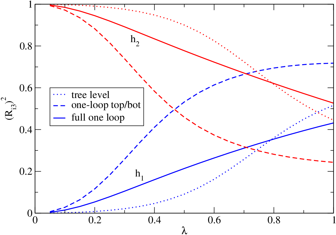
Figure 1: The squared rotation matrix element (Ri​3S)2(R^{\scriptscriptstyle S}_{i3})^{2}, measuring the singlet component in the scalars h1h_{1} and h2h_{2}, as a function of λ\lambda, for MS=300M_{S}=300 GeV. The values of the other input parameters and the meaning of the different curves are described in the text.
Refer to caption
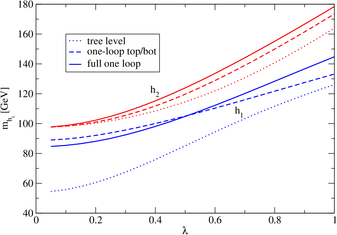
Figure 2: The masses of the two lightest scalars h1h_{1} and h2h_{2} as a function of λ\lambda, for MS=300M_{S}=300 GeV. The values of the other input parameters and the meaning of the different curves are described in the text.
Refer to caption
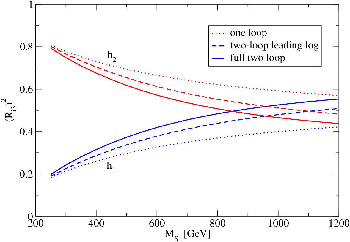
Figure 3: The squared rotation matrix element (Ri​3S)2(R^{\scriptscriptstyle S}_{i3})^{2}, measuring the singlet component in the scalars h1h_{1} and h2h_{2}, as a function of MSM_{S}, for λ=0.5\lambda=0.5. The values of the other input parameters and the meaning of the different curves are described in the text.
Refer to caption
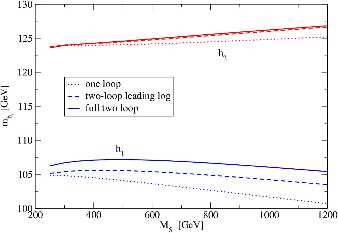
Figure 4: The masses of the two lightest scalars h1h_{1} and h2h_{2} as a function of MSM_{S}, for λ=0.5\lambda=0.5. The values of the other input parameters and the meaning of the different curves are described in the text.

Figs. 1 and 2 exemplify the effect of the one-loop corrections to the NMSSM scalar masses. In fig. 1 we plot the squared rotation matrix elements (R13S)2(R^{\scriptscriptstyle S}_{13})^{2} and (R23S)2(R^{\scriptscriptstyle S}_{23})^{2}, which measure the strength of the singlet component in the two lightest scalars h1h_{1} and h2h_{2}, as a function of λ\lambda for MS=300M_{S}=300 GeV. In fig. 2 we plot the masses of the two lightest scalars for the same choices of inputs. In both plots, the dotted lines correspond to the tree-level results; the dashed lines include the one-loop 𝒪⁡(αt){\cal O}(\alpha_{t}) and 𝒪⁡(αb){\cal O}(\alpha_{b}) corrections computed in the effective potential approach; finally, the solid lines correspond to the results of the full one-loop calculation. For the full one-loop calculation of the rotation matrix the external momentum in the scalar self energies is set to zero. It can be seen in fig. 1 that, at small λ\lambda, the lightest scalar h1h_{1} is dominantly MSSM-like while h2h_{2} is dominantly singlet. When λ\lambda increases the mixing between singlet and lightest MSSM-like Higgs increases as well. Meanwhile, the heaviest scalar h3h_{3} has a mass of the order of 600 GeV and its singlet component is always small. It is interesting to note that – at least in this point of the parameter space – the value of λ\lambda for which the two lightest mass eigenstates cross over (i.e., h1h_{1} becomes dominantly singlet) depends quite strongly on the accuracy of the calculation. In particular, when only the quark/squark contributions to the radiative corrections are included the crossover occurs for much lower values of λ\lambda than in the full one-loop calculation. Fig. 2 shows the effect of the radiative corrections to the two lightest scalar masses. The rise with λ\lambda in the tree-level masses is due to the well-known NMSSM contribution to the Higgs quartic coupling proportional to λ2​sin2⁡2​β\lambda^{2}\sin^{2}2\beta. The comparison between the dotted and dashed lines shows that the 𝒪⁡(αt){\cal O}(\alpha_{t}) corrections induced by top and stop loops have a particularly large effect on mh1m_{h_{1}} for small values of λ\lambda, when h1h_{1} is light and mostly MSSM-like. The 𝒪⁡(αb){\cal O}(\alpha_{b}) corrections induced by bottom and sbottom loops are also included in the dashed lines, but they are negligible due to the small value of tan⁡β\tan\beta. When λ\lambda increases the 𝒪⁡(αt){\cal O}(\alpha_{t}) corrections are shared between mh1m_{h_{1}} and mh2m_{h_{2}}, and become less relevant due to the increase in the tree-level masses. However, even for the heavier scalar h2h_{2} these corrections can still amount to several GeV at large λ\lambda. Finally, the comparison between the solid and dashed lines in fig. 2 shows that the remaining one-loop corrections – which constitute one of the original contributions of this paper – are also relevant, and can account for shifts of 5–10 GeV in both masses.

Figs. 3 and 4 exemplify the effect of the two-loop corrections to the NMSSM scalar masses. In fig. 3 we plot (R13S)2(R^{\scriptscriptstyle S}_{13})^{2} and (R23S)2(R^{\scriptscriptstyle S}_{23})^{2} as a function of MSM_{S} for λ=0.5\lambda=0.5. In fig. 4 we plot the masses of the two lightest scalars for the same choices of inputs. In both plots, the dotted lines corresponds to the full one-loop results (again, the rotation matrix is computed at zero external momentum); the dashed lines include the two-loop leading-logarithmic 𝒪⁡(αt​αs){\cal O}(\alpha_{t}\alpha_{s}) contribution to the (2,2) entry of the scalar mass matrix as implemented in NMHDECAY [30], i.e.

(Δ​ℳS2)22LL=6​αt​αsπ2​mt2​log2​MS2mt2.\left(\Delta{\cal M}^{2}_{S}\right)_{22}^{\rm LL}~=~6\,\frac{\alpha_{t}\alpha_{s}}{\pi^{2}}\,m_{t}^{2}\,\log^{2}\frac{M_{S}^{2}}{m_{t}^{2}}~. (44)

Finally, the solid lines correspond to the results of our two-loop 𝒪⁡(αt​αs+αb​αs){\cal O}(\alpha_{t}\alpha_{s}+\alpha_{b}\alpha_{s}) calculation. It can be seen in fig. 3 that for small MSM_{S} the lightest scalar h1h_{1} is mostly MSSM-like while h2h_{2} is mostly singlet. When MSM_{S} increases, the radiative corrections increase the mixing between singlet and MSSM-like Higgs. Fig. 4 shows that the two-loop corrections to the lightest scalar mass are positive and relatively small. This is a typical feature of the DR¯\overline{\rm DR} computation, in contrast to the OS computation in which the two-loop corrections are negative and much larger (for a discussion of this issue in the MSSM see ref. [35]). It is interesting to note that, in this scenario, the leading-logarithmic term accounts only for a fraction (30% to 60%, increasing with MSM_{S}) of the total 𝒪⁡(αt​αs){\cal O}(\alpha_{t}\alpha_{s}) contribution to the (2,2) entry of the scalar mass matrix. Indeed, the leading-logarithmic approximation of eq. (44) neglects potentially large contributions controlled by powers of the ratio At/MSA_{t}/M_{S}, as well as the possibility of mass splittings among stops and gluino. The effect of the 𝒪⁡(αt​αs){\cal O}(\alpha_{t}\alpha_{s}) corrections to the entries of the scalar mass matrix other than (2,2) is also non-negligible. The comparison between the dashed and solid curves for h1h_{1} in figs. 3 and 4 shows that, in this point of the parameter space, the non-leading-logarithmic contributions contained in our two-loop calculation induce a shift of 1–2 GeV in mh1m_{h_{1}}, and have a sizeable effect on the mixing matrix as well (on the other hand, the near overlap of the dashed and solid curves for h2h_{2} in fig. 4 is the result of an accidental cancellation). One of the attractive features of the NMSSM is the viability of scenarios in which MSM_{S} is not much above the weak scale. It is clear from figs. 3 and 4 that, in those scenarios, the leading-logarithmic approximation is not satisfactory, and a reliable evaluation of the two-loop corrections requires at least the complete 𝒪⁡(αt​αs+αb​αs){\cal O}(\alpha_{t}\alpha_{s}+\alpha_{b}\alpha_{s}) calculation.

Refer to caption
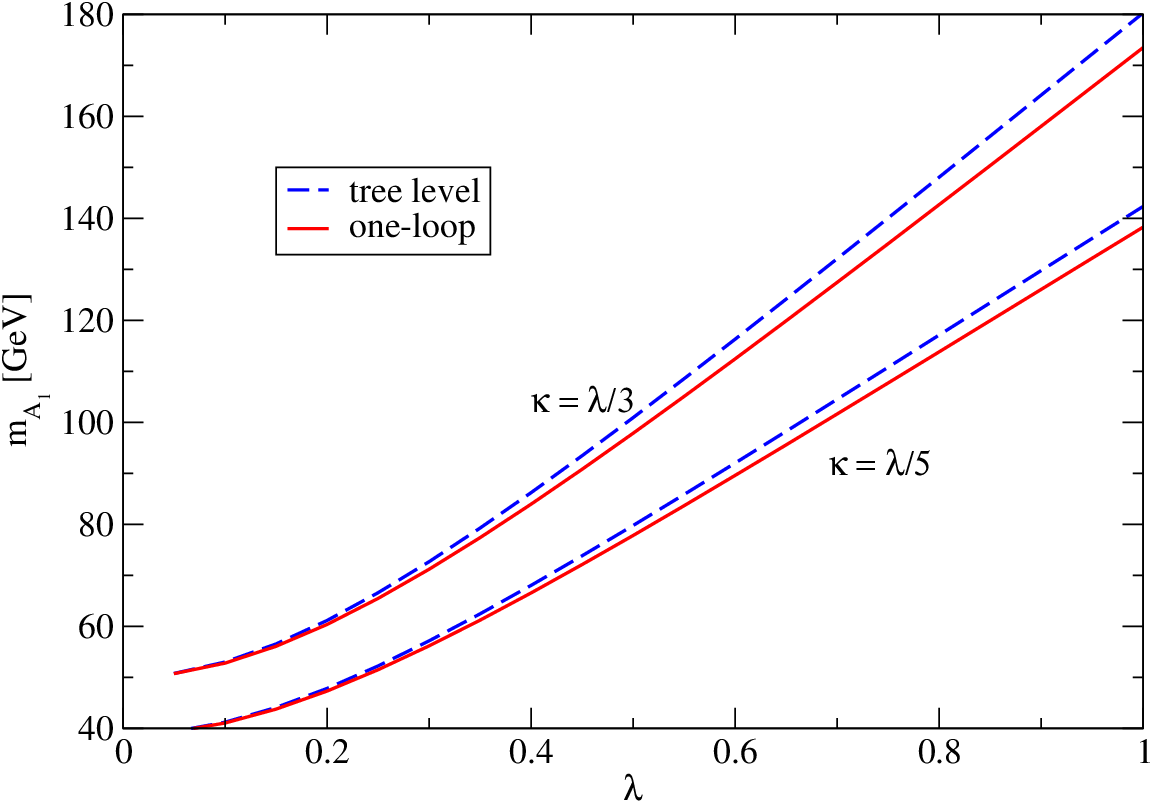
Figure 5: The masses of the lightest physical pseudoscalar A1A_{1} as a function of λ\lambda, for MS=300M_{S}=300 GeV and κ\kappa set equal to either λ/5\lambda/5 or λ/3\lambda/3. The values of the other input parameters and the meaning of the different curves are described in the text.

To conclude this section, we show in fig. 5 the effect of the radiative corrections to the mass of the lightest physical pseudoscalar A1A_{1}. For the choice of parameters considered in this example A1A_{1} is almost entirely singlet, therefore its mass is hardly affected by the one- and two-loop corrections involving quark/squark loops. The pseudoscalar A2A_{2}, on the other hand, is almost entirely MSSM-like, but its tree-level mass is of the order of 600 GeV, thus it is also not much affected by the radiative corrections. However, the Higgs self-interactions and the Higgs-higgsino interactions controlled by the superpotential couplings λ\lambda and κ\kappa do induce non-negligible corrections to the lightest pseudoscalar mass. The dashed and solid lines in fig. 5 correspond to the tree-level and one-loop determinations of mA1m_{A_{1}}, respectively, as a function of λ\lambda. The input parameters are chosen as in eqs. (42) and (43), but we show two sets of curves corresponding to κ=λ/5\kappa=\lambda/5 and κ=λ/3\kappa=\lambda/3. From the comparison between the dashed and solid curves it can be seen that the one-loop corrections to mA1m_{A_{1}} can amount to several GeV when λ\lambda and κ\kappa take on relatively large values. The two-loop corrections computed in this paper include only the quark/squark contributions, therefore the corresponding curves would essentially overlap with the one-loop curves.

6 Conclusions

The NMSSM is an attractive extension of the MSSM: it provides an elegant solution to the μ\mu problem, it reduces the need for heavy superpartners to lift the Higgs mass through radiative corrections and it has an interesting collider phenomenology. However, the accuracy of the theoretical predictions for the NMSSM Higgs masses has until now been stuck to the level that for the MSSM had been achieved in the mid-1990s. In this paper we took a few steps towards bridging the accuracy gap between the NMSSM and MSSM calculations. In particular, we provided a full one-loop calculation of the self energies and tadpoles of the neutral Higgs bosons of the NMSSM, and we computed the two-loop 𝒪⁡(αt​αs+αb​αs){\cal O}(\alpha_{t}\alpha_{s}+\alpha_{b}\alpha_{s}) corrections to the neutral Higgs boson masses in the effective potential approximation. We showed that both classes of corrections can induce shifts of a few GeV in the light scalar and pseudoscalar masses, and they can also sizeably affect the mixing between singlet and MSSM-like Higgs scalars. Taking these corrections into account in phenomenological analyses of the NMSSM Higgs sector will be crucial for a meaningful comparison between the MSSM and NMSSM predictions.

Acknowledgments

We thank F. Boudjema for discussions. This work was supported in part by an EU Marie-Curie Research Training Network under contract MRTN-CT-2006-035505 and by ANR under contract BLAN07-2_194882.

Appendix A: definitions of the couplings

In this appendix we provide explicit formulae for the couplings that enter the calculation of the one-loop corrections to the Higgs boson masses in the NMSSM.

Higgs–sfermion couplings:

the terms in the NMSSM Lagrangian relevant to the calculation of the sfermion contributions to the Higgs self energies can be written as

ℒ⊃−∑i​j​k​ℓλsi​sj​F~k​F~ℓSiSjF~∗kF~ℓ−∑i​j​k​ℓλpi​pj​F~k​F~ℓPiPjF~∗kF~ℓ−∑i​k​ℓλsi​F~k​F~ℓSiF~∗kF~ℓ−∑i​k​ℓiλpi​F~k​F~ℓPiF~∗kF~ℓ,{\cal L}~\supset~-\sum_{ijk\ell}\lambda_{s_{i}s_{j}\tilde{F}_{k}\tilde{F}_{\ell}}~S_{i}S_{j}\tilde{F}^{*}_{k}\tilde{F}_{\ell}~-\sum_{ijk\ell}\lambda_{p_{i}p_{j}\tilde{F}_{k}\tilde{F}_{\ell}}~P_{i}P_{j}\tilde{F}^{*}_{k}\tilde{F}_{\ell}~-\sum_{ik\ell}\lambda_{s_{i}\tilde{F}_{k}\tilde{F}_{\ell}}~S_{i}\tilde{F}^{*}_{k}\tilde{F}_{\ell}~-\sum_{ik\ell}i\,\lambda_{p_{i}\tilde{F}_{k}\tilde{F}_{\ell}}~P_{i}\tilde{F}^{*}_{k}\tilde{F}_{\ell}~, (A1)

where F~i=(f~L,f~R)\tilde{F}_{i}=(\tilde{f}_{L},\tilde{f}_{R}) represent the sfermions in the basis of interaction eigenstates. The quartic couplings in eq. (A1) are symmetric with respect to the exchange of ii and jj as well as with respect to the exchange of kk and ℓ\ell. The trilinear couplings of the scalars are symmetric with respect to the exchange of kk and ℓ\ell, whereas the trilinear couplings of the pseudoscalars are antisymmetric. The couplings to up-type and down-type squarks (the generalization to the sleptons is straightforward) are

λs1​s1​U~1​U~1=λp1​p1​U~1​U~1=g¯22​guL,λs1​s1​U~2​U~2=λp1​p1​U~2​U~2=g¯22​guR,\lambda_{s_{1}s_{1}\tilde{U}_{1}\tilde{U}_{1}}~=~\lambda_{p_{1}p_{1}\tilde{U}_{1}\tilde{U}_{1}}~=~\frac{\bar{g}^{2}}{2}\,g_{u_{L}}\,,~~~~~~\lambda_{s_{1}s_{1}\tilde{U}_{2}\tilde{U}_{2}}~=~\lambda_{p_{1}p_{1}\tilde{U}_{2}\tilde{U}_{2}}~=~\frac{\bar{g}^{2}}{2}\,g_{u_{R}}\,,
λs2​s2​U~1​U~1=λp2​p2​U~1​U~1=−g¯22​guL+hu22,λs2​s2​U~2​U~2=λp2​p2​U~2​U~2=−g¯22​guR+hu22,\lambda_{s_{2}s_{2}\tilde{U}_{1}\tilde{U}_{1}}~=~\lambda_{p_{2}p_{2}\tilde{U}_{1}\tilde{U}_{1}}~=~-\frac{\bar{g}^{2}}{2}\,g_{u_{L}}~+~\frac{h_{u}^{2}}{2}\,,~~~~~~\lambda_{s_{2}s_{2}\tilde{U}_{2}\tilde{U}_{2}}~=~\lambda_{p_{2}p_{2}\tilde{U}_{2}\tilde{U}_{2}}~=~-\frac{\bar{g}^{2}}{2}\,g_{u_{R}}~+~\frac{h_{u}^{2}}{2}\,,
λs1​s3​U~1​U~2=−λp1​p3​U~1​U~2=−hu​λ4,\lambda_{s_{1}s_{3}\tilde{U}_{1}\tilde{U}_{2}}~=~-\lambda_{p_{1}p_{3}\tilde{U}_{1}\tilde{U}_{2}}~=~-\frac{h_{u}\,\lambda}{4}~, (A2)
λs1​s1​D~1​D~1=λp1​p1​D~1​D~1=g¯22​gdL+hd22,λs1​s1​D~2​D~2=λp1​p1​D~2​D~2=g¯22​gdR+hd22,\lambda_{s_{1}s_{1}\tilde{D}_{1}\tilde{D}_{1}}~=~\lambda_{p_{1}p_{1}\tilde{D}_{1}\tilde{D}_{1}}~=~\frac{\bar{g}^{2}}{2}\,g_{d_{L}}~+~\frac{h_{d}^{2}}{2}\,,~~~~~~\lambda_{s_{1}s_{1}\tilde{D}_{2}\tilde{D}_{2}}~=~\lambda_{p_{1}p_{1}\tilde{D}_{2}\tilde{D}_{2}}~=~\frac{\bar{g}^{2}}{2}\,g_{d_{R}}~+~\frac{h_{d}^{2}}{2}\,,
λs2​s2​D~1​D~1=λp2​p2​D~1​D~1=−g¯22​gdL,λs2​s2​D~2​D~2=λp2​p2​D~2​D~2=−g¯22​gdR,\lambda_{s_{2}s_{2}\tilde{D}_{1}\tilde{D}_{1}}~=~\lambda_{p_{2}p_{2}\tilde{D}_{1}\tilde{D}_{1}}~=~-\frac{\bar{g}^{2}}{2}\,g_{d_{L}}\,,~~~~~~\lambda_{s_{2}s_{2}\tilde{D}_{2}\tilde{D}_{2}}~=~\lambda_{p_{2}p_{2}\tilde{D}_{2}\tilde{D}_{2}}~=~-\frac{\bar{g}^{2}}{2}\,g_{d_{R}}\,,
λs2​s3​D~1​D~2=−λp2​p3​D~1​D~2=−hd​λ4,\lambda_{s_{2}s_{3}\tilde{D}_{1}\tilde{D}_{2}}~=~-\lambda_{p_{2}p_{3}\tilde{D}_{1}\tilde{D}_{2}}~=~-\frac{h_{d}\,\lambda}{4}~, (A3)
λs1​U~1​U~1=2​g¯2​guL​v1,λs1​U~2​U~2=2​g¯2​guR​v1,\lambda_{s_{1}\tilde{U}_{1}\tilde{U}_{1}}~=~\sqrt{2}\,\bar{g}^{2}\,g_{u_{L}}\,v_{1}\,,~~~~~~\lambda_{s_{1}\tilde{U}_{2}\tilde{U}_{2}}~=~\sqrt{2}\,\bar{g}^{2}\,g_{u_{R}}\,v_{1}\,,
λs2​U~1​U~1=−2​g¯2​guL​v2+2​hu2​v2,λs2​U~2​U~2=−2​g¯2​guR​v2+2​hu2​v2,\lambda_{s_{2}\tilde{U}_{1}\tilde{U}_{1}}~=~-\sqrt{2}\,\bar{g}^{2}\,g_{u_{L}}\,v_{2}~+~\sqrt{2}\,h_{u}^{2}\,v_{2}\,,~~~~~~\lambda_{s_{2}\tilde{U}_{2}\tilde{U}_{2}}~=~-\sqrt{2}\,\bar{g}^{2}\,g_{u_{R}}\,v_{2}~+~\sqrt{2}\,h_{u}^{2}\,v_{2}\,,
λs1​U~1​U~2=λp1​U~2​U~1=−hu​vs​λ2,λs2​U~1​U~2=λp2​U~1​U~2=hu​Au2,λs3​U~1​U~2=λp3​U~2​U~1=−hu​v1​λ2,\lambda_{s_{1}\tilde{U}_{1}\tilde{U}_{2}}=\lambda_{p_{1}\tilde{U}_{2}\tilde{U}_{1}}\,=\,-\frac{h_{u}\,v_{s}\,\lambda}{\sqrt{2}}\,,~~~~\lambda_{s_{2}\tilde{U}_{1}\tilde{U}_{2}}=\lambda_{p_{2}\tilde{U}_{1}\tilde{U}_{2}}\,=\,\frac{h_{u}\,A_{u}}{\sqrt{2}}\,,~~~~\lambda_{s_{3}\tilde{U}_{1}\tilde{U}_{2}}=\lambda_{p_{3}\tilde{U}_{2}\tilde{U}_{1}}\,=\,-\frac{h_{u}\,v_{1}\,\lambda}{\sqrt{2}}~, (A4)
λs1​D~1​D~1=2​g¯2​gdL​v1+2​hd2​v1,λs1​D~2​D~2=2​g¯2​gdR​v1+2​hd2​v1,\lambda_{s_{1}\tilde{D}_{1}\tilde{D}_{1}}~=~\sqrt{2}\,\bar{g}^{2}\,g_{d_{L}}\,v_{1}~+~\sqrt{2}\,h_{d}^{2}\,v_{1}\,,~~~~~~\lambda_{s_{1}\tilde{D}_{2}\tilde{D}_{2}}~=~\sqrt{2}\,\bar{g}^{2}\,g_{d_{R}}\,v_{1}~+~\sqrt{2}\,h_{d}^{2}\,v_{1}\,,
λs2​D~1​D~1=−2​g¯2​gdL​v2,λs2​D~2​D~2=−2​g¯2​gdR​v2,\lambda_{s_{2}\tilde{D}_{1}\tilde{D}_{1}}~=~-\sqrt{2}\,\bar{g}^{2}\,g_{d_{L}}\,v_{2}\,,~~~~~~\lambda_{s_{2}\tilde{D}_{2}\tilde{D}_{2}}~=~-\sqrt{2}\,\bar{g}^{2}\,g_{d_{R}}\,v_{2}\,,
λs1​D~1​D~2=λp1​D~1​D~2=hd​Ad2,λs2​D~1​D~2=λp2​D~2​D~1=−hd​vs​λ2,λs3​D~1​D~2=λp3​D~2​D~1=−hd​v2​λ2,\lambda_{s_{1}\tilde{D}_{1}\tilde{D}_{2}}=\lambda_{p_{1}\tilde{D}_{1}\tilde{D}_{2}}\,=\,\frac{h_{d}\,A_{d}}{\sqrt{2}}\,,~~~~\lambda_{s_{2}\tilde{D}_{1}\tilde{D}_{2}}=\lambda_{p_{2}\tilde{D}_{2}\tilde{D}_{1}}\,=\,-\frac{h_{d}\,v_{s}\,\lambda}{\sqrt{2}}\,,~~~~\lambda_{s_{3}\tilde{D}_{1}\tilde{D}_{2}}=\lambda_{p_{3}\tilde{D}_{2}\tilde{D}_{1}}\,=\,-\frac{h_{d}\,v_{2}\,\lambda}{\sqrt{2}}~, (A5)

where gf=I3f−ef​sin2⁡θWg_{f}=I_{3}^{f}-e_{f}\,\sin^{2}\theta_{W}. Here I3fI_{3}^{f} is the weak isospin and efe_{f} is the electric charge of the chiral superfield that contains the sfermion (e.g., euR=−2/3e_{u_{R}}=-2/3). The couplings that cannot be obtained by swapping the last two indices and – for the quartic couplings – the first two indices of those in eqs. (A2)–(A5) are all vanishing.

In the absence of CP-violating phases in the sfermion mass matrix, the sfermion mass eigestates f~i=(f~1,f~2)\tilde{f}_{i}=(\tilde{f}_{1},\tilde{f}_{2}) are related to the interaction eigenstates F~i\tilde{F}_{i} by an orthogonal rotation:

f~i=Ri​jf​F~j,Rf=(cos⁡θfsin⁡θf−sin⁡θfcos⁡θf),\tilde{f}_{i}=R^{f}_{ij}\,\tilde{F}_{j}~,~~~~~~~~R^{f}~=~\left(\begin{array}[]{rc}\cos\theta_{f}&\sin\theta_{f}\\ -\sin\theta_{f}&\cos\theta_{f}\end{array}\right)~, (A6)

where θf\theta_{f} is the mixing angle of the sfermions f~\tilde{f}. The quartic and trilinear couplings between Higgs fields and sfermion mass eigenstates are related to the corresponding couplings between Higgs fields and sfermion interaction eigenstates as follows

λϕi​ϕj​f~k​f~ℓ=Rk​af​Rℓ​bf​λϕi​ϕj​F~a​F~b,λϕi​f~k​f~ℓ=Rk​af​Rℓ​bf​λϕi​F~a​F~b.\lambda_{\phi_{i}\phi_{j}\tilde{f}_{k}\tilde{f}_{\ell}}=R^{f}_{ka}\,R^{f}_{\ell b}\,\lambda_{\phi_{i}\phi_{j}\tilde{F}_{a}\tilde{F}_{b}}~,~~~~~~~\lambda_{\phi_{i}\tilde{f}_{k}\tilde{f}_{\ell}}=R^{f}_{ka}\,R^{f}_{\ell b}\,\lambda_{\phi_{i}\tilde{F}_{a}\tilde{F}_{b}}~. (A7)

where ϕi\phi_{i} represents either sis_{i} or pip_{i}, and summation over repeated indices is understood.

Higgs self-couplings:

the terms in the NMSSM Lagrangian relevant to the calculation of the neutral-Higgs contributions to the Higgs self energies can be written as

ℒ\displaystyle{\cal L} ⊃\displaystyle\supset −∑i​j​k​ℓλsi​sj​sk​sℓSiSjSkSℓ−∑i​j​k​ℓλpi​pj​pk​pℓPiPjPkPℓ−∑i​j​k​ℓλsi​sj​pk​pℓSiSjPkPℓ\displaystyle-\sum_{ijk\ell}\lambda_{s_{i}s_{j}s_{k}s_{\ell}}~S_{i}S_{j}S_{k}S_{\ell}~-\sum_{ijk\ell}\lambda_{p_{i}p_{j}p_{k}p_{\ell}}~P_{i}P_{j}P_{k}P_{\ell}~-\sum_{ijk\ell}\lambda_{s_{i}s_{j}p_{k}p_{\ell}}~S_{i}S_{j}P_{k}P_{\ell} (A8)
−∑i​k​ℓλsi​sk​sℓSiSkSℓ−∑i​k​ℓλsi​pk​pℓSiPkPℓ.\displaystyle-\sum_{ik\ell}\lambda_{s_{i}s_{k}s_{\ell}}~S_{i}S_{k}S_{\ell}~-\sum_{ik\ell}\lambda_{s_{i}p_{k}p_{\ell}}~S_{i}P_{k}P_{\ell}~.

The quartic and trilinear neutral-Higgs self couplings entering eq. (A8) are symmetric with respect to the permutation of any two indices corresponding to fields of the same parity. They read

λs1​s1​s1​s1=λs2​s2​s2​s2=λp1​p1​p1​p1=λp2​p2​p2​p2=g¯216,λs3​s3​s3​s3=λp3​p3​p3​p3=κ24,\lambda_{s_{1}s_{1}s_{1}s_{1}}~=~\lambda_{s_{2}s_{2}s_{2}s_{2}}~=~\lambda_{p_{1}p_{1}p_{1}p_{1}}~=~\lambda_{p_{2}p_{2}p_{2}p_{2}}~=~\frac{\bar{g}^{2}}{16}~,~~~~~~\lambda_{s_{3}s_{3}s_{3}s_{3}}~=~\lambda_{p_{3}p_{3}p_{3}p_{3}}~=~\frac{\kappa^{2}}{4}~,
λs1​s1​s2​s2=λp1​p1​p2​p2=148​(2​λ2−g¯2),λs1​s2​s3​s3=λp1​p2​p3​p3=−λ​κ24,\lambda_{s_{1}s_{1}s_{2}s_{2}}~=~\lambda_{p_{1}p_{1}p_{2}p_{2}}~=~\frac{1}{48}\,\left(2\lambda^{2}-\bar{g}^{2}\right)~,~~~~~~\lambda_{s_{1}s_{2}s_{3}s_{3}}~=~\lambda_{p_{1}p_{2}p_{3}p_{3}}~=~-\frac{\lambda\kappa}{24}~,
λs1​s1​s3​s3=λs2​s2​s3​s3=λp1​p1​p3​p3=λp2​p2​p3​p3=λ224,\lambda_{s_{1}s_{1}s_{3}s_{3}}~=~\lambda_{s_{2}s_{2}s_{3}s_{3}}~=~\lambda_{p_{1}p_{1}p_{3}p_{3}}~=~\lambda_{p_{2}p_{2}p_{3}p_{3}}~=~\frac{\lambda^{2}}{24}~,
λs1​s1​p1​p1=λs2​s2​p2​p2=g¯28,λs1​s1​p2​p2=λs2​s2​p1​p1=18​(2​λ2−g¯2),\lambda_{s_{1}s_{1}p_{1}p_{1}}~=~\lambda_{s_{2}s_{2}p_{2}p_{2}}~=~\frac{\bar{g}^{2}}{8}~,~~~~~~\lambda_{s_{1}s_{1}p_{2}p_{2}}~=~\lambda_{s_{2}s_{2}p_{1}p_{1}}~=~\frac{1}{8}\,\left(2\lambda^{2}-\bar{g}^{2}\right)~,
λs1​s1​p3​p3=λs2​s2​p3​p3=λs3​s3​p1​p1=λs3​s3​p2​p2=λ24,\lambda_{s_{1}s_{1}p_{3}p_{3}}~=~\lambda_{s_{2}s_{2}p_{3}p_{3}}~=~\lambda_{s_{3}s_{3}p_{1}p_{1}}~=~\lambda_{s_{3}s_{3}p_{2}p_{2}}~=~\frac{\lambda^{2}}{4}~,~~~~~~
λs1​s2​p3​p3=λs3​s3​p1​p2=−λs1​s3​p2​p3=−λs2​s3​p1​p3=λ​κ4,λs3​s3​p3​p3=κ22,\lambda_{s_{1}s_{2}p_{3}p_{3}}~=~\lambda_{s_{3}s_{3}p_{1}p_{2}}~=~-\lambda_{s_{1}s_{3}p_{2}p_{3}}~=~-\lambda_{s_{2}s_{3}p_{1}p_{3}}~=~\frac{\lambda\,\kappa}{4}~,~~~~~~\lambda_{s_{3}s_{3}p_{3}p_{3}}~=~\frac{\kappa^{2}}{2}~, (A9)
λs1​s1​s1=λs1​p1​p1=g¯2​v12​2,λs2​s2​s2=λs2​p2​p2=g¯2​v22​2,\lambda_{s_{1}s_{1}s_{1}}~=~\lambda_{s_{1}p_{1}p_{1}}~=~\frac{\bar{g}^{2}\,v_{1}}{2\sqrt{2}}~,~~~~~~\lambda_{s_{2}s_{2}s_{2}}~=~\lambda_{s_{2}p_{2}p_{2}}~=~\frac{\bar{g}^{2}\,v_{2}}{2\sqrt{2}}~,
λs1​p2​p2=3​λs1​s2​s2=v12​2​(2​λ2−g¯2),λs2​p1​p1=3​λs2​s1​s1=v22​2​(2​λ2−g¯2),\lambda_{s_{1}p_{2}p_{2}}~=~3\,\lambda_{s_{1}s_{2}s_{2}}~=~\frac{v_{1}}{2\sqrt{2}}\,\left(2\lambda^{2}-\bar{g}^{2}\right)~,~~~~~~\lambda_{s_{2}p_{1}p_{1}}~=~3\,\lambda_{s_{2}s_{1}s_{1}}~=~\frac{v_{2}}{2\sqrt{2}}\,\left(2\lambda^{2}-\bar{g}^{2}\right)~,
λs3​p1​p1=λs3​p2​p2=3​λs3​s1​s1=3​λs3​s2​s2=λ2​vs2,\lambda_{s_{3}p_{1}p_{1}}~=~\lambda_{s_{3}p_{2}p_{2}}~=~3\,\lambda_{s_{3}s_{1}s_{1}}~=~3\,\lambda_{s_{3}s_{2}s_{2}}~=~\frac{\lambda^{2}\,v_{s}}{\sqrt{2}}~,
λs3​s3​s3=κ​Aκ3​2+2​κ2​vs,λs3​p3​p3=−κ​Aκ2+2​κ2​vs,\lambda_{s_{3}s_{3}s_{3}}~=~\frac{\kappa\,A_{\kappa}}{3\sqrt{2}}+\sqrt{2}\,\kappa^{2}\,v_{s}~,~~~~~~\lambda_{s_{3}p_{3}p_{3}}~=~-\frac{\kappa\,A_{\kappa}}{\sqrt{2}}+\sqrt{2}\,\kappa^{2}\,v_{s}~,
λs1​s3​s3=λ3​2​(λ​v1−κ​v2),λs2​s3​s3=λ3​2​(λ​v2−κ​v1),\lambda_{s_{1}s_{3}s_{3}}~=~\frac{\lambda}{3\sqrt{2}}\,\left(\lambda\,v_{1}-\kappa v_{2}\right)~,~~~~~~\lambda_{s_{2}s_{3}s_{3}}~=~\frac{\lambda}{3\sqrt{2}}\,\left(\lambda\,v_{2}-\kappa v_{1}\right)~,~~~~~~
λs1​p3​p3=λ2​(λ​v1+κ​v2),λs2​p3​p3=λ2​(λ​v2+κ​v1),λs3​p1​p3=−λ​κ​v22,λs3​p2​p3=−λ​κ​v12,\lambda_{s_{1}p_{3}p_{3}}~=~\frac{\lambda}{\sqrt{2}}\,\left(\lambda\,v_{1}+\kappa v_{2}\right)~,~~\lambda_{s_{2}p_{3}p_{3}}~=~\frac{\lambda}{\sqrt{2}}\,\left(\lambda\,v_{2}+\kappa v_{1}\right)~,~~~\lambda_{s_{3}p_{1}p_{3}}~=~-\frac{\lambda\,\kappa\,v_{2}}{\sqrt{2}}~,~~\lambda_{s_{3}p_{2}p_{3}}~=~-\frac{\lambda\,\kappa\,v_{1}}{\sqrt{2}}~,
λs1​s2​s3=−λ​Aλ6​2−λ​κ​vs3​2,λs1​p2​p3=λs2​p1​p3=λ​Aλ2​2−λ​κ​vs2,λs3​p1​p2=λ​Aλ2​2+λ​κ​vs2.\lambda_{s_{1}s_{2}s_{3}}~=~-\frac{\lambda\,A_{\lambda}}{6\sqrt{2}}-\frac{\lambda\,\kappa\,v_{s}}{3\sqrt{2}}~,~~~~~~\lambda_{s_{1}p_{2}p_{3}}~=~\lambda_{s_{2}p_{1}p_{3}}~=~\frac{\lambda\,A_{\lambda}}{2\sqrt{2}}-\frac{\lambda\,\kappa\,v_{s}}{\sqrt{2}}~,~~~~~~\lambda_{s_{3}p_{1}p_{2}}~=~\frac{\lambda\,A_{\lambda}}{2\sqrt{2}}+\frac{\lambda\,\kappa\,v_{s}}{\sqrt{2}}~. (A10)

All of the couplings that cannot be obtained by permuting the indices of the couplings in eqs. (A9) and (A10) vanish. Rotating two scalar or pseudoscalar interaction eigenstates into mass eigenstates as in eqs. (5) and (7), and exploiting the permutation symmetry of the original couplings, the couplings that enter the calculation of the scalar self energies can be expressed as

λsi​sj​hk​hℓ=6​Rk​aS​Rℓ​bS​λsi​sj​sa​sb,λsi​sj​ak​aℓ=Rk​aP​Rℓ​bP​λsi​sj​pa​pb,\lambda_{s_{i}s_{j}h_{k}h_{\ell}}~=~6\,R^{\scriptscriptstyle S}_{ka}\,R^{\scriptscriptstyle S}_{\ell b}\,\lambda_{s_{i}s_{j}s_{a}s_{b}}~,~~~~~\lambda_{s_{i}s_{j}a_{k}a_{\ell}}~=~R^{\scriptscriptstyle P}_{ka}\,R^{\scriptscriptstyle P}_{\ell b}\,\lambda_{s_{i}s_{j}p_{a}p_{b}}~,
λsi​hk​hℓ=3​Rk​aS​Rℓ​bS​λsi​sa​sb,λsi​ak​aℓ=Rk​aP​Rℓ​bP​λsi​pa​pb.\lambda_{s_{i}h_{k}h_{\ell}}~=~3\,R^{\scriptscriptstyle S}_{ka}\,R^{\scriptscriptstyle S}_{\ell b}\,\lambda_{s_{i}s_{a}s_{b}}~,~~~~~\lambda_{s_{i}a_{k}a_{\ell}}~=~R^{\scriptscriptstyle P}_{ka}\,R^{\scriptscriptstyle P}_{\ell b}\,\lambda_{s_{i}p_{a}p_{b}}~. (A11)

Similarly, the couplings that enter the calculation of the pseudoscalar self energies are

λpi​pj​ak​aℓ=6​Rk​aP​Rℓ​bP​λpi​pj​pa​pb,λpi​pj​hk​hℓ=Rk​aS​Rℓ​bS​λsa​sb​pi​pj,\lambda_{p_{i}p_{j}a_{k}a_{\ell}}~=~6\,R^{\scriptscriptstyle P}_{ka}\,R^{\scriptscriptstyle P}_{\ell b}\,\lambda_{p_{i}p_{j}p_{a}p_{b}}~,~~~~~\lambda_{p_{i}p_{j}h_{k}h_{\ell}}=R^{\scriptscriptstyle S}_{ka}\,R^{\scriptscriptstyle S}_{\ell b}\,\lambda_{s_{a}s_{b}p_{i}p_{j}}~,
λpi​ak​hℓ=2​Rℓ​aS​Rk​bP​λsa​pb​pi.\lambda_{p_{i}a_{k}h_{\ell}}~=~2\,R^{\scriptscriptstyle S}_{\ell a}\,R^{\scriptscriptstyle P}_{kb}\,\lambda_{s_{a}p_{b}p_{i}}~. (A12)

The terms in the NMSSM Lagrangian relevant to the calculation of the charged-Higgs contributions to the Higgs self energies can be written as

ℒ\displaystyle{\cal L} ⊃\displaystyle\supset −∑i​j​k​ℓλsi​sj​hk+​hℓ−SiSjh+kh−ℓ−∑i​j​k​ℓλpi​pj​hk+​hℓ−PiPjh+kh−ℓ\displaystyle-\sum_{ijk\ell}\lambda_{s_{i}s_{j}h^{+}_{k}h^{-}_{\ell}}~S_{i}S_{j}h^{+}_{k}h^{-}_{\ell}~-\sum_{ijk\ell}\lambda_{p_{i}p_{j}h^{+}_{k}h^{-}_{\ell}}~P_{i}P_{j}h^{+}_{k}h^{-}_{\ell} (A13)
−∑i​k​ℓλsi​hk+​hℓ−Sih+kh−ℓ−∑i​k​ℓiλpi​hk+​hℓ−Pih+kh−ℓ,\displaystyle-\sum_{ik\ell}\lambda_{s_{i}h^{+}_{k}h^{-}_{\ell}}~S_{i}h^{+}_{k}h^{-}_{\ell}~-\sum_{ik\ell}i\,\lambda_{p_{i}h^{+}_{k}h^{-}_{\ell}}~P_{i}h^{+}_{k}h^{-}_{\ell}~,

where we express the charged Higgs fields directly in the basis of mass eigenstates, so hi±h_{i}^{\pm} stands for (G±,H±)(G^{\pm},H^{\pm}). In our conventions the relation between the charged Higgs mass eigenstates and interaction eigenstates reads 44 4 This differs from the conventions of Ref. [12] by one field redefinition.

(G±H±)=RC​(H1±H2±),RC=(−cos⁡βsin⁡βsin⁡βcos⁡β).\left(\begin{array}[]{c}G^{\pm}\\ H^{\pm}\end{array}\right)~=~R^{\scriptscriptstyle C}\,\left(\begin{array}[]{c}H_{1}^{\pm}\\ H_{2}^{\pm}\end{array}\right)~,~~~~~R^{\scriptscriptstyle C}~=~\left(\begin{array}[]{rc}-\cos\beta&\sin\beta\\ \sin\beta&\cos\beta\end{array}\right)~. (A14)

The quartic couplings in eq. (A13) are symmetric with respect to the exchange of ii and jj as well as with respect to the exchange of kk and ℓ\ell. The trilinear couplings of the scalars are symmetric with respect to the exchange of kk and ℓ\ell, whereas the trilinear couplings of the pseudoscalars are antisymmetric. Explicit expressions for the couplings are

λs1​s1​h1+​h1−=λs2​s2​h2+​h2−=λp1​p1​h1+​h1−=λp2​p2​h2+​h2−=18​(g2+g′ 2​cos⁡2​β),\lambda_{s_{1}s_{1}h_{1}^{+}h_{1}^{-}}~=~\lambda_{s_{2}s_{2}h_{2}^{+}h_{2}^{-}}~=~\lambda_{p_{1}p_{1}h_{1}^{+}h_{1}^{-}}~=~\lambda_{p_{2}p_{2}h_{2}^{+}h_{2}^{-}}~=~\frac{1}{8}\,(g^{2}+g^{\prime\,2}\cos 2\beta)~,
λs1​s1​h2+​h2−=λs2​s2​h1+​h1−=λp1​p1​h2+​h2−=λp2​p2​h1+​h1−=18​(g2−g′ 2​cos⁡2​β),\lambda_{s_{1}s_{1}h_{2}^{+}h_{2}^{-}}~=~\lambda_{s_{2}s_{2}h_{1}^{+}h_{1}^{-}}~=~\lambda_{p_{1}p_{1}h_{2}^{+}h_{2}^{-}}~=~\lambda_{p_{2}p_{2}h_{1}^{+}h_{1}^{-}}~=~\frac{1}{8}\,(g^{2}-g^{\prime\,2}\cos 2\beta)~,
λs1​s2​h1+​h1−=λp1​p2​h2+​h2−=−λs1​s2​h2+​h2−=−λp1​p2​h1+​h1−=18​(2​λ2−g2)​sin⁡2​β,\lambda_{s_{1}s_{2}h_{1}^{+}h_{1}^{-}}~=~\lambda_{p_{1}p_{2}h_{2}^{+}h_{2}^{-}}~=~-\lambda_{s_{1}s_{2}h_{2}^{+}h_{2}^{-}}~=~-\lambda_{p_{1}p_{2}h_{1}^{+}h_{1}^{-}}~=~\frac{1}{8}\,(2\lambda^{2}-g^{2})\,\sin 2\beta~,
λs1​s1​h1+​h2−=λp1​p1​h1+​h2−=−λs2​s2​h1+​h2−=−λp2​p2​h1+​h2−=−g′ 28​sin⁡2​β,\lambda_{s_{1}s_{1}h_{1}^{+}h_{2}^{-}}~=~\lambda_{p_{1}p_{1}h_{1}^{+}h_{2}^{-}}~=~-\lambda_{s_{2}s_{2}h_{1}^{+}h_{2}^{-}}~=~-\lambda_{p_{2}p_{2}h_{1}^{+}h_{2}^{-}}~=~-\frac{\;g^{\prime\,2}}{8}\,\sin 2\beta~,
λs1​s2​h1+​h2−=−λp1​p2​h1+​h2−=18​(2​λ2−g2)​cos⁡2​β,λs3​s3​h1+​h2−=−λp3​p3​h1+​h2−=−κ​λ2​cos⁡2​β,\lambda_{s_{1}s_{2}h_{1}^{+}h_{2}^{-}}~=~-\lambda_{p_{1}p_{2}h_{1}^{+}h_{2}^{-}}~=~\frac{1}{8}\,(2\lambda^{2}-g^{2})\,\cos 2\beta~,~~~~~\lambda_{s_{3}s_{3}h_{1}^{+}h_{2}^{-}}~=~-\lambda_{p_{3}p_{3}h_{1}^{+}h_{2}^{-}}~=~-\frac{\kappa\lambda}{2}\,\cos 2\beta~,
λs3​s3​h1+​h1−=λp3​p3​h2+​h2−=λ2​(λ−κ​sin⁡2​β),λs3​s3​h2+​h2−=λp3​p3​h1+​h1−=λ2​(λ+κ​sin⁡2​β),\lambda_{s_{3}s_{3}h_{1}^{+}h_{1}^{-}}~=~\lambda_{p_{3}p_{3}h_{2}^{+}h_{2}^{-}}~=~\frac{\lambda}{2}\,(\lambda-\kappa\,\sin 2\beta)~,~~~~~\lambda_{s_{3}s_{3}h_{2}^{+}h_{2}^{-}}~=~\lambda_{p_{3}p_{3}h_{1}^{+}h_{1}^{-}}~=~\frac{\lambda}{2}\,(\lambda+\kappa\,\sin 2\beta)~, (A15)
λs1​h1+​h1−=12​2​(v1​(g2+g′ 2​cos⁡2​β)+v2​(2​λ2−g2)​sin⁡2​β),\lambda_{s_{1}h_{1}^{+}h_{1}^{-}}~=~\frac{1}{2\sqrt{2}}\,\left(v_{1}\,(g^{2}+g^{\prime\,2}\cos 2\beta)~+~v_{2}\,(2\lambda^{2}-g^{2})\,\sin 2\beta\right)~,
λs1​h2+​h2−=12​2​(v1​(g2−g′ 2​cos⁡2​β)−v2​(2​λ2−g2)​sin⁡2​β),\lambda_{s_{1}h_{2}^{+}h_{2}^{-}}~=~\frac{1}{2\sqrt{2}}\,\left(v_{1}\,(g^{2}-g^{\prime\,2}\cos 2\beta)~-~v_{2}\,(2\lambda^{2}-g^{2})\,\sin 2\beta\right)~,
λs1​h1+​h2−=12​2​(−v1​g′ 2​sin⁡2​β+v2​(2​λ2−g2)​cos⁡2​β),\lambda_{s_{1}h_{1}^{+}h_{2}^{-}}~=~\frac{1}{2\sqrt{2}}\,\left(-v_{1}\,g^{\prime\,2}\sin 2\beta~+~v_{2}\,(2\lambda^{2}-g^{2})\,\cos 2\beta\right)~,
λs2​h1+​h1−=12​2​(v2​(g2−g′ 2​cos⁡2​β)+v1​(2​λ2−g2)​sin⁡2​β),\lambda_{s_{2}h_{1}^{+}h_{1}^{-}}~=~\frac{1}{2\sqrt{2}}\,\left(v_{2}\,(g^{2}-g^{\prime\,2}\cos 2\beta)~+~v_{1}\,(2\lambda^{2}-g^{2})\,\sin 2\beta\right)~,
λs2​h2+​h2−=12​2​(v2​(g2+g′ 2​cos⁡2​β)−v1​(2​λ2−g2)​sin⁡2​β),\lambda_{s_{2}h_{2}^{+}h_{2}^{-}}~=~\frac{1}{2\sqrt{2}}\,\left(v_{2}\,(g^{2}+g^{\prime\,2}\cos 2\beta)~-~v_{1}\,(2\lambda^{2}-g^{2})\,\sin 2\beta\right)~,
λs2​h1+​h2−=12​2​(v2​g′ 2​sin⁡2​β+v1​(2​λ2−g2)​cos⁡2​β),\lambda_{s_{2}h_{1}^{+}h_{2}^{-}}~=~\frac{1}{2\sqrt{2}}\,\left(v_{2}\,g^{\prime\,2}\sin 2\beta~+~v_{1}\,(2\lambda^{2}-g^{2})\,\cos 2\beta\right)~,
λs3​h1+​h1−=λ2​(2​λ​vs−(Aλ+2​κ​vs)​sin⁡2​β),λs3​h2+​h2−=λ2​(2​λ​vs+(Aλ+2​κ​vs)​sin⁡2​β),\lambda_{s_{3}h_{1}^{+}h_{1}^{-}}~=~\frac{\lambda}{\sqrt{2}}\,\left(2\lambda\,v_{s}-(A_{\lambda}+2\kappa\,v_{s})\,\sin 2\beta\right)~,~~~~\lambda_{s_{3}h_{2}^{+}h_{2}^{-}}~=~\frac{\lambda}{\sqrt{2}}\,\left(2\lambda\,v_{s}+(A_{\lambda}+2\kappa\,v_{s})\,\sin 2\beta\right)~,
λs3​h1+​h2−=−λ2​(Aλ+2​κ​vs)​cos⁡2​β,\lambda_{s_{3}h_{1}^{+}h_{2}^{-}}~=~-\frac{\lambda}{\sqrt{2}}\,(A_{\lambda}+2\kappa\,v_{s})\,\cos 2\beta~,
λp1​h1+​h2−=v22​2​(2​λ2−g2),λp2​h1+​h2−=v12​2​(2​λ2−g2),λp3​h1+​h2−=λ2​(Aλ−2​κ​vs).\lambda_{p_{1}h_{1}^{+}h_{2}^{-}}~=~\frac{v_{2}}{2\sqrt{2}}\,(2\lambda^{2}-g^{2})~,~~~~\lambda_{p_{2}h_{1}^{+}h_{2}^{-}}~=~\frac{v_{1}}{2\sqrt{2}}\,(2\lambda^{2}-g^{2})~,~~~~\lambda_{p_{3}h_{1}^{+}h_{2}^{-}}~=~\frac{\lambda}{\sqrt{2}}\,(A_{\lambda}-2\kappa\,v_{s})~. (A16)

All of the couplings that cannot be obtained by permuting the indices of the couplings in eqs. (A15) and (A16) vanish.

Higgs–neutralino couplings:

In the formalism of two component spinors, the terms in the NMSSM Lagrangian relevant to the calculation of the neutralino contributions to the Higgs self energies can be written as

ℒ⊃−∑i​k​ℓλsi​ψk0​ψℓ0Siψ0kψ0ℓ−i∑i​k​ℓλpi​ψk0​ψℓ0Piψ0kψ0ℓ+h.c.,{\cal L}~\supset~-\sum_{ik\ell}\lambda_{s_{i}\psi^{0}_{k}\psi^{0}_{\ell}}~S_{i}\,\psi^{0}_{k}\psi^{0}_{\ell}~-~i\,\sum_{ik\ell}\lambda_{p_{i}\psi^{0}_{k}\psi^{0}_{\ell}}~P_{i}\,\psi^{0}_{k}\psi^{0}_{\ell}~~+~{\rm h.c.}~, (A17)

where ψi0=(−i​b~,−i​w~0,h~10,h~20,s~)\psi^{0}_{i}=(-i\tilde{b},\,-i\tilde{w}^{0},\,\tilde{h}_{1}^{0},\,\tilde{h}_{2}^{0},\,\tilde{s}) are the neutralino interaction eigenstates. The couplings in eq. (A17) are symmetric with respect to the exchange of the neutralino indices kk and ℓ\ell, and read

λs1​ψ10​ψ30=−λs2​ψ10​ψ40=−λp1​ψ10​ψ30=λp2​ψ10​ψ40=−g′4,\lambda_{s_{1}\psi^{0}_{1}\psi^{0}_{3}}~=~-\lambda_{s_{2}\psi^{0}_{1}\psi^{0}_{4}}~=~-\lambda_{p_{1}\psi^{0}_{1}\psi^{0}_{3}}~=~\lambda_{p_{2}\psi^{0}_{1}\psi^{0}_{4}}~=~-\frac{\,g^{\prime}}{4}~,
λs1​ψ20​ψ30=−λs2​ψ20​ψ40=−λp1​ψ20​ψ30=λp2​ψ20​ψ40=g4,λs3​ψ50​ψ50=λp3​ψ50​ψ50=κ2,\lambda_{s_{1}\psi^{0}_{2}\psi^{0}_{3}}~=~-\lambda_{s_{2}\psi^{0}_{2}\psi^{0}_{4}}~=~-\lambda_{p_{1}\psi^{0}_{2}\psi^{0}_{3}}~=~\lambda_{p_{2}\psi^{0}_{2}\psi^{0}_{4}}~=~\frac{g}{4}~,~~~~~~~\lambda_{s_{3}\psi^{0}_{5}\psi^{0}_{5}}~=~\lambda_{p_{3}\psi^{0}_{5}\psi^{0}_{5}}~=~\frac{\kappa}{\sqrt{2}}~,
λs1​ψ40​ψ50=λs2​ψ30​ψ50=λs3​ψ30​ψ40=λp1​ψ40​ψ50=λp2​ψ30​ψ50=λp3​ψ30​ψ40=−λ2​2.\lambda_{s_{1}\psi^{0}_{4}\psi^{0}_{5}}~=~\lambda_{s_{2}\psi^{0}_{3}\psi^{0}_{5}}~=~\lambda_{s_{3}\psi^{0}_{3}\psi^{0}_{4}}~=~\lambda_{p_{1}\psi^{0}_{4}\psi^{0}_{5}}~=~\lambda_{p_{2}\psi^{0}_{3}\psi^{0}_{5}}~=~\lambda_{p_{3}\psi^{0}_{3}\psi^{0}_{4}}~=~-\frac{\lambda}{2\sqrt{2}}~. (A18)

All of the couplings that cannot be obtained by permuting the neutralino indices of the couplings in the equation above vanish. The couplings of the Higgs bosons to the neutralino mass eigenstates χi0\chi_{i}^{0} are related to the corresponding couplings to the neutralino interaction eigenstates as follows

λϕi​χk0​χℓ0=Nk​a∗​Nℓ​b∗​λϕi​ψa0​ψb0,\lambda_{\phi_{i}\chi^{0}_{k}\chi^{0}_{\ell}}=N^{*}_{ka}\,N^{*}_{\ell b}\,\lambda_{\phi_{i}\psi^{0}_{a}\psi^{0}_{b}}~, (A19)

where ϕi\phi_{i} represents either sis_{i} or pip_{i}, NN is the rotation matrix defined in eq. (9) and summation over repeated indices is understood. In the absence of CP-violating phases in the neutralino mass matrix, the couplings can be taken as real if we allow for negative neutralino masses.

Higgs–chargino couplings:

The terms in the NMSSM Lagrangian relevant to the calculation of the chargino contributions to the Higgs self energies can be written as

ℒ⊃−∑i​k​ℓλsi​ψk+​ψℓ−Siψ+kψ−ℓ−i∑i​k​ℓλpi​ψk+​ψℓ−Piψ+kψ−ℓ+h.c.,{\cal L}~\supset~-\sum_{ik\ell}\lambda_{s_{i}\psi^{+}_{k}\psi^{-}_{\ell}}~S_{i}\,\psi^{+}_{k}\psi^{-}_{\ell}~-~i\,\sum_{ik\ell}\lambda_{p_{i}\psi^{+}_{k}\psi^{-}_{\ell}}~P_{i}\,\psi^{+}_{k}\psi^{-}_{\ell}~~+~{\rm h.c.}~, (A20)

where ψi+=(−i​w~+,h~2+)\psi^{+}_{i}=(-i\tilde{w}^{+},\,\,\tilde{h}_{2}^{+}) and ψi−=(−i​w~−,h~1−)\psi^{-}_{i}=(-i\tilde{w}^{-},\,\,\tilde{h}_{1}^{-}) are the positive and negative chargino interaction eigenstates, respectively, in the formalism of two-component spinors. The only non-zero couplings in eq. (A20) are

λs1​ψ1+​ψ2−=λs2​ψ2+​ψ1−=−λp1​ψ1+​ψ2−=−λp2​ψ2+​ψ1−=g2,\lambda_{s_{1}\psi^{+}_{1}\psi^{-}_{2}}~=~\lambda_{s_{2}\psi^{+}_{2}\psi^{-}_{1}}~=~-\lambda_{p_{1}\psi^{+}_{1}\psi^{-}_{2}}~=~-\lambda_{p_{2}\psi^{+}_{2}\psi^{-}_{1}}~=~\frac{g}{\sqrt{2}}~,
λs3​ψ2+​ψ2−=λp3​ψ2+​ψ2−=λ2.\lambda_{s_{3}\psi^{+}_{2}\psi^{-}_{2}}~=~\lambda_{p_{3}\psi^{+}_{2}\psi^{-}_{2}}~=~\frac{\lambda}{\sqrt{2}}~. (A21)

The mass matrix ℳχ{\cal M}_{\chi} for the charginos can be diagonalized by a biunitary transformation

diag⁡(mχi+)=U∗​ℳχ​V†,{\rm diag}(m_{\chi^{+}_{i}})=U^{*}\,{\cal M}_{\chi}V^{\dagger}~, (A22)

where the unitary matrices UU and VV rotate the negative and positive chargino interaction eigenstates, respectively, into the corresponding mass eigenstates

χi−=Ui​j​ψj−,χi+=Vi​j​ψj+.\chi^{-}_{i}~=~U_{ij}\,\psi^{-}_{j}~,~~~~~~~\chi^{+}_{i}~=~V_{ij}\,\psi^{+}_{j}~. (A23)

The couplings of the Higgs bosons to the chargino mass eigenstates are related to the corresponding couplings to the chargino interaction eigenstates as follows

λϕi​χk+​χℓ−=Vk​a∗​Uℓ​b∗​λϕi​ψa+​ψb−,\lambda_{\phi_{i}\chi^{+}_{k}\chi^{-}_{\ell}}=V^{*}_{ka}\,U^{*}_{\ell b}\,\lambda_{\phi_{i}\psi^{+}_{a}\psi^{-}_{b}}~, (A24)

where ϕi\phi_{i} represents either sis_{i} or pip_{i} and summation over repeated indices is understood. In the absence of CP-violating phases in the chargino mass matrix, the couplings can be taken as real if we allow for negative chargino masses.

ZZ–neutralino and ZZ–chargino couplings:

Since the singlino is neutral with respect to the MSSM gauge sector, the couplings of the ZZ boson to the neutralinos (and, of course, to the charginos) in the interaction basis are the same as in the MSSM. In the formalism of two-component spinors they read

ℒ⊃−∑i​j(λZ​ψi0​ψj0Zμψ¯i0σ¯μψj0+h.c.)−∑i​jλZ​ψi+​ψj+Zμψ¯i+σ¯μψj+−∑i​jλZ​ψi−​ψj−Zμψi−σμψ¯j−.{\cal L}~\supset~-\sum_{ij}\left(\lambda_{Z\psi^{0}_{i}\psi^{0}_{j}}\,Z_{\mu}\,\bar{\psi}^{0}_{i}\bar{\sigma}^{\mu}\psi^{0}_{j}~+~{\rm h.c.}\right)~-~\sum_{ij}\lambda_{Z\psi^{+}_{i}\psi^{+}_{j}}\,Z_{\mu}\,\bar{\psi}^{+}_{i}\bar{\sigma}^{\mu}\psi^{+}_{j}~-~\sum_{ij}\lambda_{Z\psi^{-}_{i}\psi^{-}_{j}}\,Z_{\mu}\,\psi^{-}_{i}\sigma^{\mu}\bar{\psi}^{-}_{j}~. (A25)

The only non-zero couplings are

λZ​ψ30​ψ30=−λZ​ψ40​ψ40=g¯2​2,λZ​ψ1+​ψ1+=λZ​ψ1−​ψ1−=g22​g¯,λZ​ψ2+​ψ2+=λZ​ψ2−​ψ2−=g¯2​cos⁡2​θW.\lambda_{Z\psi^{0}_{3}\psi^{0}_{3}}~=\,-\lambda_{Z\psi^{0}_{4}\psi^{0}_{4}}~=~\frac{\bar{g}}{2\sqrt{2}}~,~~~~\lambda_{Z\psi^{+}_{1}\psi^{+}_{1}}~=\,\lambda_{Z\psi^{-}_{1}\psi^{-}_{1}}~=~\frac{g^{2}}{\sqrt{2}\,\bar{g}}~,~~~~\lambda_{Z\psi^{+}_{2}\psi^{+}_{2}}~=\,\lambda_{Z\psi^{-}_{2}\psi^{-}_{2}}~=~\frac{\bar{g}}{\sqrt{2}}\,\cos 2\theta_{\scriptscriptstyle W}~. (A26)

In terms of the neutralino and chargino mass eigenstates, the couplings read

λZ​χi0​χj0=Ni​k​Nj​ℓ∗​λZ​ψk0​ψℓ0,λZ​χi+​χj+=Vi​k​Vj​ℓ∗​λZ​ψk+​ψℓ+,λZ​χi−​χj−=Ui​k∗​Uj​ℓ​λZ​ψk−​ψℓ−.\lambda_{Z\chi^{0}_{i}\chi^{0}_{j}}=N_{ik}N^{*}_{j\ell}\,\lambda_{Z\psi^{0}_{k}\psi^{0}_{\ell}}~,~~~~~~\lambda_{Z\chi^{+}_{i}\chi^{+}_{j}}=V_{ik}V^{*}_{j\ell}\,\lambda_{Z\psi^{+}_{k}\psi^{+}_{\ell}}~,~~~~~~\lambda_{Z\chi^{-}_{i}\chi^{-}_{j}}=U^{*}_{ik}U_{j\ell}\,\lambda_{Z\psi^{-}_{k}\psi^{-}_{\ell}}~. (A27)

WW–neutralino–chargino couplings:

The couplings of the WW boson with charginos and neutralinos are the same as in the MSSM, but we give them for completeness. In the formalism of two-component spinors, they read

ℒ⊃−∑i​jλW​ψi0​ψj+W+μψ¯+jσ¯μψ0i−∑i​jλZ​ψi0​ψj−W+μψ−jσμψ¯0i+h.c.{\cal L}~\supset~-\sum_{ij}\lambda_{W\psi^{0}_{i}\psi^{+}_{j}}\,W^{+}_{\mu}\,\bar{\psi}^{+}_{j}\bar{\sigma}^{\mu}\psi^{0}_{i}~-\sum_{ij}\lambda_{Z\psi^{0}_{i}\psi^{-}_{j}}\,W^{+}_{\mu}\,\psi^{-}_{j}\sigma^{\mu}\bar{\psi}^{0}_{i}~+~{\rm h.c.} (A28)

The only non-zero couplings are

λW​ψ20​ψ1+=λW​ψ20​ψ1−=−g,λW​ψ40​ψ2+=−λW​ψ30​ψ2−=g2,\lambda_{W\psi^{0}_{2}\psi^{+}_{1}}~=\,\lambda_{W\psi^{0}_{2}\psi^{-}_{1}}~=~-\,g~,~~~~\lambda_{W\psi^{0}_{4}\psi^{+}_{2}}~=\,-\lambda_{W\psi^{0}_{3}\psi^{-}_{2}}~=~\frac{g}{\sqrt{2}}~,~~~~ (A29)

In terms of the neutralino and chargino mass eigenstates, the couplings read

λW​χi0​χj+=Ni​k∗​Vj​ℓ​λW​ψk0​ψℓ+,λW​χi0​χj−=Ni​k​Uj​ℓ∗​λZ​ψk0​ψℓ−.\lambda_{W\chi^{0}_{i}\chi^{+}_{j}}=N^{*}_{ik}V_{j\ell}\,\lambda_{W\psi^{0}_{k}\psi^{+}_{\ell}}~,~~~~~~\lambda_{W\chi^{0}_{i}\chi^{-}_{j}}=N_{ik}U^{*}_{j\ell}\,\lambda_{Z\psi^{0}_{k}\psi^{-}_{\ell}}~. (A30)

Appendix B: one-loop self energies and tadpoles

In this appendix we list the explicit formulae for the one-loop self energies and tadpole diagrams that are necessary to the calculation of the neutral Higgs boson masses. The calculation is performed in the ’t Hooft-Feynman gauge, in which the Goldstone bosons and the ghosts have the same masses as the corresponding gauge bosons.

Scalar self energies

The contributions to the scalar self energies from matter-fermion loops and from loops involving gauge bosons or ghosts are essentially the same as in the MSSM, and read [12]

16​π2​Πs1​s1f,V​(p2)\displaystyle 16\,\pi^{2}\,\Pi_{s_{1}s_{1}}^{f,\,V}(p^{2}) =\displaystyle= 3​hb2​[(p2−4​mb2)​B0​(mb,mb)−2​A0​(mb)]\displaystyle 3\,h_{b}^{2}\,\left[(p^{2}-4\,m_{b}^{2})\,B_{0}(m_{b},m_{b})-2\,A_{0}(m_{b})\right] (B1)
+\displaystyle+ hτ2​[(p2−4​mτ2)​B0​(mτ,mτ)−2​A0​(mτ)]\displaystyle~\;h_{\tau}^{2}\,\left[(p^{2}-4\,m_{\tau}^{2})\,B_{0}(m_{\tau},m_{\tau})-2\,A_{0}(m_{\tau})\right]
+\displaystyle+ g22​∑i=12(Ri​1C)2​F​(mhi±,MW)+g¯22​∑i=13(Ri​1P)2​F​(mai,MZ)\displaystyle\frac{g^{2}}{2}\,\sum_{i=1}^{2}\,\left(R^{\scriptscriptstyle C}_{i1}\right)^{2}\,F(m_{h^{\pm}_{i}},M_{W})~+~\frac{\bar{g}^{2}}{2}\,\sum_{i=1}^{3}\,\left(R^{\scriptscriptstyle P}_{i1}\right)^{2}\,F(m_{a_{i}},M_{Z})
+\displaystyle+ 72​cβ2​[g2​MW2​B0​(MW,MW)+g¯2​MZ2​B0​(MZ,MZ)]\displaystyle\frac{7}{2}\,c_{\beta}^{2}\,\left[g^{2}\,M_{W}^{2}\,B_{0}(M_{W},M_{W})+\bar{g}^{2}\,M_{Z}^{2}\,B_{0}(M_{Z},M_{Z})\right]
+\displaystyle+ 2​g2​A0​(MW)+2​g¯2​A0​(MZ),\displaystyle 2\,g^{2}A_{0}(M_{W})+2\,\bar{g}^{2}A_{0}(M_{Z})~,
16​π2​Πs2​s2f,V​(p2)\displaystyle 16\,\pi^{2}\,\Pi_{s_{2}s_{2}}^{f,\,V}(p^{2}) =\displaystyle= 3​ht2​[(p2−4​mt2)​B0​(mt,mt)−2​A0​(mt)]\displaystyle 3\,h_{t}^{2}\,\left[(p^{2}-4\,m_{t}^{2})\,B_{0}(m_{t},m_{t})-2\,A_{0}(m_{t})\right] (B2)
+\displaystyle+ g22​∑i=12(Ri​2C)2​F​(mhi±,MW)+g¯22​∑i=13(Ri​2P)2​F​(mai,MZ)\displaystyle\frac{g^{2}}{2}\,\sum_{i=1}^{2}\,\left(R^{\scriptscriptstyle C}_{i2}\right)^{2}\,F(m_{h^{\pm}_{i}},M_{W})~+~\frac{\bar{g}^{2}}{2}\,\sum_{i=1}^{3}\,\left(R^{\scriptscriptstyle P}_{i2}\right)^{2}\,F(m_{a_{i}},M_{Z})
+\displaystyle+ 72​sβ2​[g2​MW2​B0​(MW,MW)+g¯2​MZ2​B0​(MZ,MZ)]\displaystyle\frac{7}{2}\,s_{\beta}^{2}\,\left[g^{2}\,M_{W}^{2}\,B_{0}(M_{W},M_{W})+\bar{g}^{2}\,M_{Z}^{2}\,B_{0}(M_{Z},M_{Z})\right]
+\displaystyle+ 2​g2​A0​(MW)+2​g¯2​A0​(MZ),\displaystyle 2\,g^{2}A_{0}(M_{W})+2\,\bar{g}^{2}A_{0}(M_{Z})~,
16​π2​Πs1​s2f,V​(p2)\displaystyle 16\,\pi^{2}\,\Pi_{s_{1}s_{2}}^{f,\,V}(p^{2}) =\displaystyle= −g22∑i=12Ri​1CRi​2CF(mhi±,MW)−g¯22∑i=13Ri​1PRi​2PF(mai,MZ)\displaystyle-\frac{g^{2}}{2}\,\sum_{i=1}^{2}\,R^{\scriptscriptstyle C}_{i1}R^{\scriptscriptstyle C}_{i2}\,F(m_{h^{\pm}_{i}},M_{W})~-~\frac{\bar{g}^{2}}{2}\,\sum_{i=1}^{3}\,R^{\scriptscriptstyle P}_{i1}R^{\scriptscriptstyle P}_{i2}\,F(m_{a_{i}},M_{Z}) (B3)
+\displaystyle+ 72​sβ​cβ​[g2​MW2​B0​(MW,MW)+g¯2​MZ2​B0​(MZ,MZ)],\displaystyle\frac{7}{2}\,s_{\beta}\,c_{\beta}\,\left[g^{2}\,M_{W}^{2}\,B_{0}(M_{W},M_{W})+\bar{g}^{2}\,M_{Z}^{2}\,B_{0}(M_{Z},M_{Z})\right]~,

where we neglected the Yukawa couplings of the first two generations. The loop functions A0​(m)A_{0}(m), B0​(m1,m2)B_{0}(m_{1},m_{2}) and F⁡(m1,m2)F(m_{1},m_{2}) are defined in appendix B of ref. [12], and they depend also on the external momentum p2p^{2} and on the renormalization scale QQ. Here and in the following we use for brevity the notation cϕ≡cos⁡ϕ,sϕ≡sin⁡ϕc_{\phi}\equiv\cos\phi\,,~s_{\phi}\equiv\sin\phi, for a generic angle ϕ\phi. Also, hi±h_{i}^{\pm} stands for (G±,H±G^{\pm},H^{\pm}), aia_{i} stands for (G0,A1,A2G^{0},A_{1},A_{2}), and the rotation matrices RCR^{\scriptscriptstyle C} and RPR^{\scriptscriptstyle P} are defined in eqs. (A14) and (7), respectively. The contributions to the self energies involving the field S3S_{3} are zero because the singlet does not couple to the gauge sector nor to the matter fermions.

The sfermion contributions to the scalar self energies read

16​π2​Πsi​sjf~​(p2)=∑f~∑k=1nf~ 2​Ncf​λsi​sj​f~k​f~k​A0​(mf~k)+∑f~∑k,ℓ=1nf~Ncf​λsi​f~k​f~ℓ​λsj​f~ℓ​f~k​B0​(mf~k,mf~ℓ),16\,\pi^{2}\,\Pi_{s_{i}s_{j}}^{\tilde{f}}(p^{2})~=~\sum_{\tilde{f}}\,\sum_{k=1}^{n_{\tilde{f}}}\,2\,N_{c}^{f}\,\lambda_{s_{i}s_{j}\tilde{f}_{k}\tilde{f}_{k}}\,A_{0}(m_{\tilde{f}_{k}})~+~\sum_{\tilde{f}}\,\sum_{k,\ell=1}^{n_{\tilde{f}}}\,N_{c}^{f}\,\lambda_{s_{i}\tilde{f}_{k}\tilde{f}_{\ell}}\,\lambda_{s_{j}\tilde{f}_{\ell}\tilde{f}_{k}}\,B_{0}(m_{\tilde{f}_{k}},m_{\tilde{f}_{\ell}})~, (B4)

where the first sum in each term runs over all the sfermion species and the second over the sfermion mass eigenstates. NcfN_{c}^{f} is the number of colours for the sfermions f~\tilde{f}, while nf~n_{\tilde{f}} is 1 for the sneutrinos and 2 for all of the other sfermions. The quartic and trilinear Higgs–sfermion couplings are obtained by combining eqs. (A2)–(A7).

The Higgs contributions to the scalar self energies read

16​π2​Πsi​sjH​(p2)\displaystyle 16\,\pi^{2}\,\Pi_{s_{i}s_{j}}^{H}(p^{2}) =\displaystyle= ∑k=13 2​λsi​sj​hk​hk​A0​(mhk)+∑k,ℓ=13 2​λsi​hk​hℓ​λsj​hk​hℓ​B0​(mhk,mhℓ)\displaystyle\sum_{k=1}^{3}\,2\,\lambda_{s_{i}s_{j}h_{k}h_{k}}\,A_{0}(m_{h_{k}})+\sum_{k,\ell=1}^{3}\,2\,\lambda_{s_{i}h_{k}h_{\ell}}\,\lambda_{s_{j}h_{k}h_{\ell}}\,B_{0}(m_{h_{k}},m_{h_{\ell}}) (B5)
+\displaystyle+ ∑k=13 2​λsi​sj​ak​ak​A0​(mak)+∑k,ℓ=13 2​λsi​ak​aℓ​λsj​ak​aℓ​B0​(mak,maℓ)\displaystyle\sum_{k=1}^{3}\,2\,\lambda_{s_{i}s_{j}a_{k}a_{k}}\,A_{0}(m_{a_{k}})+\sum_{k,\ell=1}^{3}\,2\,\lambda_{s_{i}a_{k}a_{\ell}}\,\lambda_{s_{j}a_{k}a_{\ell}}\,B_{0}(m_{a_{k}},m_{a_{\ell}})
+\displaystyle+ ∑n=12 2​λsi​sj​hk+​hk−​A0​(mhk±)+∑m,n=12λsi​hk+​hℓ−​λsj​hℓ+​hk−​B0​(mhk±,mhℓ±),\displaystyle\sum_{n=1}^{2}\,2\,\lambda_{s_{i}s_{j}h^{+}_{k}h^{-}_{k}}\,A_{0}(m_{h^{\pm}_{k}})~+\sum_{m,n=1}^{2}\lambda_{s_{i}h^{+}_{k}h^{-}_{\ell}}\,\lambda_{s_{j}h^{+}_{\ell}h^{-}_{k}}\,B_{0}(m_{h^{\pm}_{k}},m_{h^{\pm}_{\ell}})~,

where the neutral couplings λsi​sj​ϕk​ϕℓ\lambda_{s_{i}s_{j}\phi_{k}\phi_{\ell}} and λsi​ϕk​ϕℓ\lambda_{s_{i}\phi_{k}\phi_{\ell}}, where ϕ\phi represents either hh or aa, are obtained by combining eqs. (A9)–(A11), while the charged couplings λsi​sj​hk+​hℓ−\lambda_{s_{i}s_{j}h^{+}_{k}h^{-}_{\ell}} and λsi​hk+​hℓ−\lambda_{s_{i}h^{+}_{k}h^{-}_{\ell}} are given in eqs. (A15) and (A16), respectively.

Finally, the chargino and neutralino contributions to the scalar self energies read

16​π2​Πsi​sjχ​(p2)\displaystyle 16\,\pi^{2}\,\Pi_{s_{i}s_{j}}^{\chi}(p^{2}) =\displaystyle= 4∑k,ℓ=15[Re(λsi​χk0​χℓ0∗λsj​χk0​χℓ0)G(mχk0,mχℓ0)\displaystyle 4\,\sum_{k,\ell=1}^{5}\,\biggr[{\rm Re}(\lambda^{*}_{s_{i}\chi^{0}_{k}\chi^{0}_{\ell}}\,\lambda_{s_{j}\chi^{0}_{k}\chi^{0}_{\ell}})\,G(m_{\chi^{0}_{k}},m_{\chi^{0}_{\ell}}) (B6)
−2mχk0mχℓ0Re(λsi​χk0​χℓ0λsj​χk0​χℓ0)B0(mχk0,mχℓ0)]\displaystyle~~~~~~~~~~~-2\,m_{\chi^{0}_{k}}\,m_{\chi^{0}_{\ell}}\,{\rm Re}(\lambda_{s_{i}\chi^{0}_{k}\chi^{0}_{\ell}}\,\lambda_{s_{j}\chi^{0}_{k}\chi^{0}_{\ell}})\,B_{0}(m_{\chi^{0}_{k}},m_{\chi^{0}_{\ell}})\biggr]
+\displaystyle+ 2∑k,ℓ=12[Re(λsi​χk+​χℓ−∗λsj​χk+​χℓ−)G(mχk±,mχℓ±)\displaystyle 2\,\sum_{k,\ell=1}^{2}\,\biggr[{\rm Re}(\lambda^{*}_{s_{i}\chi^{+}_{k}\chi^{-}_{\ell}}\,\lambda_{s_{j}\chi^{+}_{k}\chi^{-}_{\ell}})\,G(m_{\chi^{\pm}_{k}},m_{\chi^{\pm}_{\ell}})
−2mχk±mχℓ±Re(λsi​χk+​χℓ−λsj​χℓ+​χk−)B0(mχk±,mχℓ±)],\displaystyle~~~~~~~~~~~-2\,m_{\chi^{\pm}_{k}}\,m_{\chi^{\pm}_{\ell}}\,{\rm Re}(\lambda_{s_{i}\chi^{+}_{k}\chi^{-}_{\ell}}\,\lambda_{s_{j}\chi^{+}_{\ell}\chi^{-}_{k}})\,B_{0}(m_{\chi^{\pm}_{k}},m_{\chi^{\pm}_{\ell}})\biggr]~,

where the loop function G⁡(m1,m2)G(m_{1},m_{2}) is defined in appendix B of ref. [12], the Higgs-neutralino couplings are obtained by combining eqs. (A18) and (A19), and the Higgs-chargino couplings are obtained by combining eqs. (A21) and (A24).

Pseudoscalar self energies

The contributions to the pseudoscalar self energies from matter-fermion loops and from loops involving gauge bosons or ghosts read

16​π2​Πp1​p1f,V​(p2)\displaystyle 16\,\pi^{2}\,\Pi_{p_{1}p_{1}}^{f,\,V}(p^{2}) =\displaystyle= 3​hb2​[p2​B0​(mb,mb)−2​A0​(mb)]+hτ2​[p2​B0​(mτ,mτ)−2​A0​(mτ)]\displaystyle 3\,h_{b}^{2}\,\left[p^{2}\,B_{0}(m_{b},m_{b})-2\,A_{0}(m_{b})\right]~+~h_{\tau}^{2}\,\left[p^{2}\,B_{0}(m_{\tau},m_{\tau})-2\,A_{0}(m_{\tau})\right] (B7)
+\displaystyle+ g22​∑i=12(Ri​1C)2​F​(mhi±,MW)+g¯22​∑i=13(Ri​1S)2​F​(mhi,MZ)\displaystyle\frac{g^{2}}{2}\,\sum_{i=1}^{2}\,\left(R^{\scriptscriptstyle C}_{i1}\right)^{2}\,F(m_{h^{\pm}_{i}},M_{W})~+~\frac{\bar{g}^{2}}{2}\,\sum_{i=1}^{3}\,\left(R^{\scriptscriptstyle S}_{i1}\right)^{2}\,F(m_{h_{i}},M_{Z})
+\displaystyle+ g22​cβ2​MW2​B0​(MW,MW)+2​g2​A0​(MW)+2​g¯2​A0​(MZ),\displaystyle\frac{g^{2}}{2}\,c_{\beta}^{2}\,M_{W}^{2}\,B_{0}(M_{W},M_{W})+2\,g^{2}A_{0}(M_{W})+2\,\bar{g}^{2}A_{0}(M_{Z})~,
16​π2​Πp2​p2f,V​(p2)\displaystyle 16\,\pi^{2}\,\Pi_{p_{2}p_{2}}^{f,\,V}(p^{2}) =\displaystyle= 3​ht2​[p2​B0​(mt,mt)−2​A0​(mt)]\displaystyle 3\,h_{t}^{2}\,\left[p^{2}\,B_{0}(m_{t},m_{t})-2\,A_{0}(m_{t})\right] (B8)
+\displaystyle+ g22​∑i=12(Ri​2C)2​F​(mhi±,MW)+g¯22​∑i=13(Ri​2S)2​F​(mhi,MZ)\displaystyle\frac{g^{2}}{2}\,\sum_{i=1}^{2}\,\left(R^{\scriptscriptstyle C}_{i2}\right)^{2}\,F(m_{h^{\pm}_{i}},M_{W})~+~\frac{\bar{g}^{2}}{2}\,\sum_{i=1}^{3}\,\left(R^{\scriptscriptstyle S}_{i2}\right)^{2}\,F(m_{h_{i}},M_{Z})
+\displaystyle+ g22​sβ2​MW2​B0​(MW,MW)+2​g2​A0​(MW)+2​g¯2​A0​(MZ),\displaystyle\frac{g^{2}}{2}\,s_{\beta}^{2}\,M_{W}^{2}\,B_{0}(M_{W},M_{W})+2\,g^{2}A_{0}(M_{W})+2\,\bar{g}^{2}A_{0}(M_{Z})~,
16​π2​Πp1​p2f,V​(p2)\displaystyle 16\,\pi^{2}\,\Pi_{p_{1}p_{2}}^{f,\,V}(p^{2}) =\displaystyle= g22​∑i=12Ri​1C​Ri​2C​F​(mhi±,MW)−g¯22​∑i=13Ri​1S​Ri​2S​F​(mhi,MZ)\displaystyle\frac{g^{2}}{2}\,\sum_{i=1}^{2}\,R^{\scriptscriptstyle C}_{i1}R^{\scriptscriptstyle C}_{i2}\,F(m_{h^{\pm}_{i}},M_{W})-\frac{\bar{g}^{2}}{2}\,\sum_{i=1}^{3}\,R^{\scriptscriptstyle S}_{i1}R^{\scriptscriptstyle S}_{i2}\,F(m_{h_{i}},M_{Z}) (B9)
−\displaystyle- g22​cβ​sβ​MW2​B0​(MW,MW),\displaystyle\frac{g^{2}}{2}\,c_{\beta}\,s_{\beta}\,M_{W}^{2}\,B_{0}(M_{W},M_{W})~,

the rotation matrices RCR^{\scriptscriptstyle C} and RSR^{\scriptscriptstyle S} are defined in eqs. (A14) and (5), respectively. The contributions to the self energies involving the field P3P_{3} are zero because the singlet does not couple to the gauge sector nor to the matter fermions.

The sfermion contributions to the pseudoscalar self energies read

16​π2​Πpi​pjf~​(p2)=∑f~∑k=1nf~ 2​Ncf​λpi​pj​f~k​f~k​A0​(mf~k)−∑f~∑k,ℓ=1nf~Ncf​λpi​f~k​f~ℓ​λpj​f~ℓ​f~k​B0​(mf~k,mf~ℓ),16\,\pi^{2}\,\Pi_{p_{i}p_{j}}^{\tilde{f}}(p^{2})~=~\sum_{\tilde{f}}\,\sum_{k=1}^{n_{\tilde{f}}}\,2\,N_{c}^{f}\,\lambda_{p_{i}p_{j}\tilde{f}_{k}\tilde{f}_{k}}\,A_{0}(m_{\tilde{f}_{k}})~-~\sum_{\tilde{f}}\,\sum_{k,\ell=1}^{n_{\tilde{f}}}\,N_{c}^{f}\,\lambda_{p_{i}\tilde{f}_{k}\tilde{f}_{\ell}}\,\lambda_{p_{j}\tilde{f}_{\ell}\tilde{f}_{k}}\,B_{0}(m_{\tilde{f}_{k}},m_{\tilde{f}_{\ell}})~, (B10)

where the quartic and trilinear Higgs–sfermion couplings are obtained by combining eqs. (A2)–(A7).

The Higgs contributions to the pseudoscalar self energies read

16​π2​Πpi​pjH​(p2)\displaystyle 16\,\pi^{2}\,\Pi_{p_{i}p_{j}}^{H}(p^{2}) =\displaystyle= ∑k=13 2​λpi​pj​hk​hk​A0​(mhk)+∑k=13 2​λpi​pj​ak​ak​A0​(mak)\displaystyle\sum_{k=1}^{3}\,2\,\lambda_{p_{i}p_{j}h_{k}h_{k}}\,A_{0}(m_{h_{k}})+\sum_{k=1}^{3}\,2\,\lambda_{p_{i}p_{j}a_{k}a_{k}}\,A_{0}(m_{a_{k}}) (B11)
+\displaystyle+ ∑k,ℓ=13λpi​ak​hℓ​λpj​ak​hℓ​B0​(mak,mhℓ)\displaystyle\sum_{k,\ell=1}^{3}\,\lambda_{p_{i}a_{k}h_{\ell}}\,\lambda_{p_{j}a_{k}h_{\ell}}\,B_{0}(m_{a_{k}},m_{h_{\ell}})
+\displaystyle+ ∑n=12 2​λpi​pj​hk+​hk−​A0​(mhk±)−∑m,n=12λpi​hk+​hℓ−​λpj​hℓ+​hk−​B0​(mhk±,mhℓ±),\displaystyle\sum_{n=1}^{2}\,2\,\lambda_{p_{i}p_{j}h^{+}_{k}h^{-}_{k}}\,A_{0}(m_{h^{\pm}_{k}})~-\sum_{m,n=1}^{2}\lambda_{p_{i}h^{+}_{k}h^{-}_{\ell}}\,\lambda_{p_{j}h^{+}_{\ell}h^{-}_{k}}\,B_{0}(m_{h^{\pm}_{k}},m_{h^{\pm}_{\ell}})~,

where the neutral couplings λpi​pj​hk​hℓ\lambda_{p_{i}p_{j}h_{k}h_{\ell}}, λpi​pj​ak​aℓ\lambda_{p_{i}p_{j}a_{k}a_{\ell}} and λpi​ak​hℓ\lambda_{p_{i}a_{k}h_{\ell}} are obtained by combining eqs. (A9) and (A10) with eq. (A12), while the charged couplings λpi​pj​hk+​hℓ−\lambda_{p_{i}p_{j}h^{+}_{k}h^{-}_{\ell}} and λpi​hk+​hℓ−\lambda_{p_{i}h^{+}_{k}h^{-}_{\ell}} are given in eqs. (A15) and (A16), respectively.

Finally, the chargino and neutralino contributions to the pseudoscalar self energies read

16​π2​Πpi​pjχ​(p2)\displaystyle 16\,\pi^{2}\,\Pi_{p_{i}p_{j}}^{\chi}(p^{2}) =\displaystyle= 4∑k,ℓ=15[Re(λpi​χk0​χℓ0∗λpj​χk0​χℓ0)G(mχk0,mχℓ0)\displaystyle 4\,\sum_{k,\ell=1}^{5}\,\biggr[{\rm Re}(\lambda^{*}_{p_{i}\chi^{0}_{k}\chi^{0}_{\ell}}\,\lambda_{p_{j}\chi^{0}_{k}\chi^{0}_{\ell}})\,G(m_{\chi^{0}_{k}},m_{\chi^{0}_{\ell}}) (B12)
+2mχk0mχℓ0Re(λpi​χk0​χℓ0λpj​χk0​χℓ0)B0(mχk0,mχℓ0)]\displaystyle~~~~~~~~~~~+2\,m_{\chi^{0}_{k}}\,m_{\chi^{0}_{\ell}}\,{\rm Re}(\lambda_{p_{i}\chi^{0}_{k}\chi^{0}_{\ell}}\,\lambda_{p_{j}\chi^{0}_{k}\chi^{0}_{\ell}})\,B_{0}(m_{\chi^{0}_{k}},m_{\chi^{0}_{\ell}})\biggr]
+\displaystyle+ 2∑k,ℓ=12[Re(λpi​χk+​χℓ−∗λpj​χk+​χℓ−)G(mχk±,mχℓ±)\displaystyle 2\,\sum_{k,\ell=1}^{2}\,\biggr[{\rm Re}(\lambda^{*}_{p_{i}\chi^{+}_{k}\chi^{-}_{\ell}}\,\lambda_{p_{j}\chi^{+}_{k}\chi^{-}_{\ell}})\,G(m_{\chi^{\pm}_{k}},m_{\chi^{\pm}_{\ell}})
+2mχk±mχℓ±Re(λpi​χk+​χℓ−λpj​χℓ+​χk−)B0(mχk±,mχℓ±)],\displaystyle~~~~~~~~~~~+2\,m_{\chi^{\pm}_{k}}\,m_{\chi^{\pm}_{\ell}}\,{\rm Re}(\lambda_{p_{i}\chi^{+}_{k}\chi^{-}_{\ell}}\,\lambda_{p_{j}\chi^{+}_{\ell}\chi^{-}_{k}})\,B_{0}(m_{\chi^{\pm}_{k}},m_{\chi^{\pm}_{\ell}})\biggr]~,

where the Higgs-neutralino couplings are obtained by combining eqs. (A18) and (A19), and the Higgs-chargino couplings are obtained by combining eqs. (A21) and (A24).

Scalar tadpoles

The contributions to the scalar tadpoles from matter-fermion loops and from loops involving gauge bosons or ghosts are the same as in the MSSM, and read [12]

16​π2​T1f,V\displaystyle 16\,\pi^{2}\,T_{1}^{\,f,\,V} =\displaystyle= −6​2​hb​mb​A0​(mb)−2​2​hτ​mτ​A0​(mτ)+3​v12​(g2​A0​(MW)+g¯2​A0​(MZ)),\displaystyle-6\,\sqrt{2}\,h_{b}\,m_{b}\,A_{0}(m_{b})-2\,\sqrt{2}\,h_{\tau}\,m_{\tau}\,A_{0}(m_{\tau})+\frac{3\,v_{1}}{\sqrt{2}}\left(g^{2}\,A_{0}(M_{W})+\bar{g}^{2}\,A_{0}(M_{Z})\right)~,
16​π2​T2f,V\displaystyle 16\,\pi^{2}\,T_{2}^{\,f,\,V} =\displaystyle= −6​2​ht​mt​A0​(mt)+3​v22​(g2​A0​(MW)+g¯2​A0​(MZ)).\displaystyle-6\,\sqrt{2}\,h_{t}\,m_{t}\,A_{0}(m_{t})+\frac{3\,v_{2}}{\sqrt{2}}\left(g^{2}\,A_{0}(M_{W})+\bar{g}^{2}\,A_{0}(M_{Z})\right)~. (B14)

The contributions to T3T_{3} are zero because the singlet does not couple to the gauge sector nor to the matter fermions.

The contributions to the tadpoles from loops involving sfermions or Higgs bosons read

16​π2​Tif~,ϕ=∑f~∑k=1nf~Ncf​λsi​f~k​f~k​A0​(mf~k)+∑ϕ∑k=1nϕλsi​ϕk​ϕk​A0​(mϕ~k),16\,\pi^{2}\,T_{i}^{\tilde{f}\,,\phi}~=~\sum_{\tilde{f}}\,\sum_{k=1}^{n_{\tilde{f}}}\,N_{c}^{f}\,\lambda_{s_{i}\tilde{f}_{k}\tilde{f}_{k}}\,A_{0}(m_{\tilde{f}_{k}})~+~\sum_{\phi}\,\sum_{k=1}^{n_{\phi}}\,\,\lambda_{s_{i}\phi_{k}\phi_{k}}\,A_{0}(m_{\tilde{\phi}_{k}})~, (B15)

where the first sum in the second term runs over all the Higgs bosons (i.e., ϕ=h,a,h±\phi=h,a,h^{\pm}), and nϕn_{\phi} is 2 for h±h^{\pm} and 3 for hh and aa. The trilinear Higgs–sfermion couplings are obtained by combining eqs. (A4)–(A7); the trilinear neutral-Higgs self-couplings are obtained by combining eqs. (A10) and (A11); the trilinear couplings with the charged Higgs bosons are given in eq. (A16).

Finally, the contributions to the tadpoles from loops involving neutralinos or charginos read

16π2Tiχ=−4∑k=15λsi​χk0​χk0mχk0A0(mχk0)−4∑k=12λsi​χk+​χk−mχk±A0(mχk±),16\,\pi^{2}\,T_{i}^{\chi}~=~-4\,\sum_{k=1}^{5}\,\lambda_{s_{i}\chi^{0}_{k}\chi^{0}_{k}}\,m_{\chi^{0}_{k}}\,A_{0}(m_{\chi^{0}_{k}})~-4\,\sum_{k=1}^{2}\,\lambda_{s_{i}\chi^{+}_{k}\chi^{-}_{k}}\,m_{\chi^{\pm}_{k}}\,A_{0}(m_{\chi^{\pm}_{k}})~, (B16)

where the Higgs-neutralino couplings are obtained by combining eqs. (A18) and (A19), and the Higgs-chargino couplings are obtained by combining eqs. (A21) and (A24).

Vector boson self energies

Since the singlet superfield is neutral under the MSSM gauge group, the vector boson self energies in the NMSSM differ from the corresponding MSSM quantities only through the effect of the mixing of the singlet and singlino with the MSSM Higgs bosons and higgsinos, respectively. The transverse parts of the WW and ZZ self energies appearing in eqs. (14) and (15) can be obtained by inserting in eqs. (D.4) and (D.9) of ref. [12] appropriate combinations of the Higgs scalar and pseudoscalar mixing matrices, as well as the chargino and neutralino couplings defined in appendix A.

The transverse part of the ZZ-boson self energy reads

16​π2​ΠZ​ZT​(p2)\displaystyle 16\,\pi^{2}\,\Pi^{T}_{ZZ}(p^{2}) =\displaystyle= 2​g¯2​MZ2​∑i=13(Ri​1S​cβ+Ri​2S​sβ)2​B0​(mhi,MZ)\displaystyle 2\,\bar{g}^{2}\,M_{Z}^{2}\,\sum_{i=1}^{3}\,\left(R^{\scriptscriptstyle S}_{i1}\,c_{\beta}+R^{\scriptscriptstyle S}_{i2}\,s_{\beta}\right)^{2}\,B_{0}(m_{h_{i}},M_{Z}) (B17)
−\displaystyle- 2​g¯2​∑i,j=13(Ri​1S​Rj​1P−Ri​2S​Rj​2P)2​B~22​(mhi,maj)−2​g¯2​c2​θW2​∑i2B~22​(mhi±,mhi±)\displaystyle 2\,\bar{g}^{2}\,\sum_{i,j=1}^{3}\,\left(R^{\scriptscriptstyle S}_{i1}\,R^{\scriptscriptstyle P}_{j1}-R^{\scriptscriptstyle S}_{i2}\,R^{\scriptscriptstyle P}_{j2}\right)^{2}\,\widetilde{B}_{22}(m_{h_{i}},m_{a_{j}})~-~2\,\bar{g}^{2}\,c_{2\theta_{\scriptscriptstyle W}}^{2}\,\sum_{i}^{2}\widetilde{B}_{22}(m_{h^{\pm}_{i}},m_{h^{\pm}_{i}})
−\displaystyle- 4​g¯2​cθW4​(2​p2+MW2−MZ2​sθW4cθW2)​B0​(MW,MW)−16​g¯2​cθW4​B~22​(MW,MW)\displaystyle 4\,\bar{g}^{2}\,c_{\theta_{\scriptscriptstyle W}}^{4}\,\left(2\,p^{2}+M_{W}^{2}-M_{Z}^{2}\,\frac{s_{\theta_{\scriptscriptstyle W}}^{4}}{c_{\theta_{\scriptscriptstyle W}}^{2}}\right)\,B_{0}(M_{W},M_{W})~-~16\,\bar{g}^{2}\,c_{\theta_{\scriptscriptstyle W}}^{4}\,\widetilde{B}_{22}(M_{W},M_{W})
+\displaystyle+ 2​g¯2​∑fNcf​[(gfL2+gfR2)​H​(mf,mf)−4​gfL​gfR​mf2​B0​(mf,mf)]\displaystyle 2\,\bar{g}^{2}\,\sum_{f}\,N_{c}^{f}\,\left[\left(g_{f_{L}}^{2}+g_{f_{R}}^{2}\right)\,H(m_{f},m_{f})-4\,g_{f_{L}}\,g_{f_{R}}\,m_{f}^{2}\,B_{0}(m_{f},m_{f})\right]
−\displaystyle- 8​g¯2​∑f~∑i,j=1nf~Ncf​(gfL​Ri​1f~​Rj​1f~−gfR​Ri​2f~​Rj​2f~)2​B~22​(mf~i,mf~j)\displaystyle 8\,\bar{g}^{2}\,\sum_{\tilde{f}}\sum_{i,j=1}^{n_{\tilde{f}}}\,N_{c}^{f}\,\left(g_{f_{L}}\,R^{\tilde{f}}_{i1}\,R^{\tilde{f}}_{j1}-g_{f_{R}}\,R^{\tilde{f}}_{i2}\,R^{\tilde{f}}_{j2}\right)^{2}\,\widetilde{B}_{22}(m_{\tilde{f}_{i}},m_{\tilde{f}_{j}})
+\displaystyle+ 4​∑i,j=15|λZ​χi0​χj0|2​[H⁡(mχi0,mχj0)−2​mχi0​mχj0​B0​(mχi0,mχj0)]\displaystyle 4\,\sum_{i,j=1}^{5}\,|\lambda_{Z\chi^{0}_{i}\chi^{0}_{j}}|^{2}\,\left[H(m_{\chi^{0}_{i}},m_{\chi^{0}_{j}})-2\,m_{\chi^{0}_{i}}\,m_{\chi^{0}_{j}}\,B_{0}(m_{\chi^{0}_{i}},m_{\chi^{0}_{j}})\right]
+\displaystyle+ ∑i,j=12[(|λZ​χi+​χj+|2+|λZ​χi−​χj−|2)H(mχi±,mχj±)\displaystyle\sum_{i,j=1}^{2}\,\biggr[\left(|\lambda_{Z\chi^{+}_{i}\chi^{+}_{j}}|^{2}+|\lambda_{Z\chi^{-}_{i}\chi^{-}_{j}}|^{2}\right)\,H(m_{\chi^{\pm}_{i}},m_{\chi^{\pm}_{j}})
+4mχi±mχj±Re(λZ​χi+​χj+∗λZ​χi−​χj−)B0(mχi±,mχj±)],\displaystyle~~~~~~~~~~~~~~~~~~~~+4\,m_{\chi^{\pm}_{i}}\,m_{\chi^{\pm}_{j}}\,{\rm Re}\left(\lambda_{Z\chi^{+}_{i}\chi^{+}_{j}}^{*}\lambda_{Z\chi^{-}_{i}\chi^{-}_{j}}\right)\,B_{0}(m_{\chi^{\pm}_{i}},m_{\chi^{\pm}_{j}})\biggr]~,

where the loop functions B~22​(m1,m2)\widetilde{B}_{22}(m_{1},m_{2}) and H⁡(m1,m2)H(m_{1},m_{2}) are defined in appendix B of ref. [12], gfg_{f} is defined after eq. (A5), and the couplings λZ​χi0​χj0\lambda_{Z\chi^{0}_{i}\chi^{0}_{j}}, λZ​χi+​χj+\,\lambda_{Z\chi^{+}_{i}\chi^{+}_{j}} and λZ​χi−​χj−\lambda_{Z\chi^{-}_{i}\chi^{-}_{j}} are obtained by combining eqs. (A26) and (A27).

Finally, the transverse part of the WW-boson self energy reads

16​π2​ΠW​WT​(p2)\displaystyle 16\,\pi^{2}\,\Pi^{T}_{WW}(p^{2}) =\displaystyle= g2​MW2​∑i=13(Ri​1S​cβ+Ri​2S​sβ)2​B0​(mhi,MW)\displaystyle g^{2}\,M_{W}^{2}\,\sum_{i=1}^{3}\,\left(R^{\scriptscriptstyle S}_{i1}\,c_{\beta}+R^{\scriptscriptstyle S}_{i2}\,s_{\beta}\right)^{2}\,B_{0}(m_{h_{i}},M_{W}) (B18)
−\displaystyle- g2​∑i=13∑j=12(Ri​1S​Rj​1C−Ri​2S​Rj​2C)2​B~22​(mhi,mhj±)\displaystyle g^{2}\,\sum_{i=1}^{3}\sum_{j=1}^{2}\left(R^{\scriptscriptstyle S}_{i1}\,R^{\scriptscriptstyle C}_{j1}-R^{\scriptscriptstyle S}_{i2}\,R^{\scriptscriptstyle C}_{j2}\right)^{2}\,\widetilde{B}_{22}(m_{h_{i}},m_{h^{\pm}_{j}})
−\displaystyle- g2​∑i=13∑j=12(Ri​1P​Rj​1C+Ri​2P​Rj​2C)2​B~22​(mai,mhj±)\displaystyle g^{2}\,\sum_{i=1}^{3}\sum_{j=1}^{2}\left(R^{\scriptscriptstyle P}_{i1}\,R^{\scriptscriptstyle C}_{j1}+R^{\scriptscriptstyle P}_{i2}\,R^{\scriptscriptstyle C}_{j2}\right)^{2}\,\widetilde{B}_{22}(m_{a_{i}},m_{h^{\pm}_{j}})
−\displaystyle- g2​[(4​p2+MW2+MZ2)​cθW2−MZ2​sθW4]​B0​(MZ,MW)\displaystyle g^{2}\,\left[\left(4\,p^{2}+M_{W}^{2}+M_{Z}^{2}\right)\,c_{\theta_{\scriptscriptstyle W}}^{2}-M_{Z}^{2}\,s_{\theta_{\scriptscriptstyle W}}^{4}\right]\,B_{0}(M_{Z},M_{W})
−\displaystyle- 8​g2​cθW2​B~22​(MZ,MW)−g2​sθW2​[8​B~22​(MW,0)+4​p2​B0​(MW,0)]\displaystyle 8\,g^{2}\,c_{\theta_{\scriptscriptstyle W}}^{2}\,\widetilde{B}_{22}(M_{Z},M_{W})~-~g^{2}\,s_{\theta_{\scriptscriptstyle W}}^{2}\,\left[8\,\widetilde{B}_{22}(M_{W},0)+4\,p^{2}\,B_{0}(M_{W},0)\right]
+\displaystyle+ 3​g22​∑u/dH⁡(mu,md)+g22​∑e/νH⁡(me,0)\displaystyle\frac{3\,g^{2}}{2}\,\sum_{u/d}\,H(m_{u},m_{d})~+~\frac{g^{2}}{2}\,\sum_{e/\nu}\,H(m_{e},0)
−\displaystyle- 6​g2​∑u~/d~∑i,j=12(Ri​1u~​Rj​1d~)2​B~22​(mu~i,md~j)−2​g2​∑e~/ν~∑i=12(Ri​1e~)2​B~22​(me~i,mν~)\displaystyle 6\,g^{2}\,\sum_{\tilde{u}/\tilde{d}}\,\sum_{i,j=1}^{2}\,\left(R^{\,\tilde{u}}_{i1}\,R^{\,\tilde{d}}_{j1}\right)^{2}\,\widetilde{B}_{22}(m_{\tilde{u}_{i}},m_{\tilde{d}_{j}})~-~2\,g^{2}\,\sum_{\tilde{e}/\tilde{\nu}}\,\sum_{i=1}^{2}\,\left(R^{\,\tilde{e}}_{i1}\right)^{2}\,\widetilde{B}_{22}(m_{\tilde{e}_{i}},m_{\tilde{\nu}})
+\displaystyle+ ∑i=15∑j=12[(|λW​χi0​χj+|2+|λW​χi0​χj−|2)H(mχi0,mχj±)\displaystyle\sum_{i=1}^{5}\,\sum_{j=1}^{2}\,\biggr[\left(|\lambda_{W\chi^{0}_{i}\chi^{+}_{j}}|^{2}+|\lambda_{W\chi^{0}_{i}\chi^{-}_{j}}|^{2}\right)\,H(m_{\chi^{0}_{i}},m_{\chi^{\pm}_{j}})
+4mχi0mχj±Re(λW​χi0​χj+∗λW​χi0​χj−)B0(mχi0,mχj±)],\displaystyle~~~~~~~~~~~~~~~~~~~~+4\,m_{\chi^{0}_{i}}\,m_{\chi^{\pm}_{j}}\,{\rm Re}\left(\lambda_{W\chi^{0}_{i}\chi^{+}_{j}}^{*}\lambda_{W\chi^{0}_{i}\chi^{-}_{j}}\right)\,B_{0}(m_{\chi^{0}_{i}},m_{\chi^{\pm}_{j}})\biggr]~,

where the sums in the fermion contributions and the first sums in the sfermion contributions run over the three families of (s)quarks and (s)leptons, and the couplings λW​χi0​χj+\lambda_{W\chi^{0}_{i}\chi^{+}_{j}} and λW​χi0​χj−\lambda_{W\chi^{0}_{i}\chi^{-}_{j}} are obtained by combining eqs. (A29) and (A30).

Appendix C: derivatives of the two-loop effective potential

We provide in this appendix the explicit formulae for the derivatives of the two-loop contribution to the effective potential involving top, stop, gluon and gluino. In units of αs​CF​Nc/(4​π)3\alpha_{s}\,C_{F}N_{c}\,/(4\pi)^{3}, where CF=4/3C_{F}=4/3 and Nc=3N_{c}=3 are colour factors, and in terms of the field-dependent quantities defined in eqs. (20)–(22), the 𝒪⁡(αs){\cal O}(\alpha_{s}) contribution to VeffV_{\rm eff} reads

Δ​V\displaystyle\Delta V =\displaystyle= 2​J​(mt2,mt2)−4​mt2​I​(mt2,mt2,0)+\displaystyle 2\,J(m_{t}^{2},m_{t}^{2})-4\,m_{t}^{2}\,I(m_{t}^{2},m_{t}^{2},0)+ (C1)
+\displaystyle+ {2mt~12I(mt~12,mt~12,0)+2L(mt~12,mg~2,mt2)−4mtmg~s2​θ¯cφ−φ~I(mt~12,mg~2,mt2)\displaystyle\biggr\{2\,m_{\tilde{t}_{1}}^{2}\,I(m_{\tilde{t}_{1}}^{2},m_{\tilde{t}_{1}}^{2},0)+2\,L(m_{\tilde{t}_{1}}^{2},m_{\tilde{g}}^{2},m_{t}^{2})-4\,m_{t}\,m_{\tilde{g}}\,s_{2\bar{\theta}}\,c_{\varphi-\tilde{\varphi}}\,I(m_{\tilde{t}_{1}}^{2},m_{\tilde{g}}^{2},m_{t}^{2})
+12(1+c2​θ¯2)J(mt~12,mt~12)+s2​θ¯22J(mt~12,mt~22)+[mt~1↔mt~2,s2​θ¯→−s2​θ¯]},\displaystyle+\,\frac{1}{2}\,(1+c_{2\bar{\theta}}^{2})\,J(m_{\tilde{t}_{1}}^{2},m_{\tilde{t}_{1}}^{2})+\frac{s_{2\bar{\theta}}^{2}}{2}J(m_{\tilde{t}_{1}}^{2},m_{\tilde{t}_{2}}^{2})\;\;+\;\;\left[m_{\tilde{t}_{1}}\leftrightarrow m_{\tilde{t}_{2}}\,,\,s_{2\bar{\theta}}\rightarrow-s_{2\bar{\theta}}\right]\biggr\}\,,

where the functions I,JI\,,J and LL are defined in appendix D. The derivatives of Δ​V\Delta V that involve only the field-dependent stop mixing angle θ¯\bar{\theta} and phase difference φ−φ~\varphi-\tilde{\varphi} can be straightforwardly computed from eq. (C1). In units of αs​CF​Nc/(4​π)3\alpha_{s}\,C_{F}N_{c}\,/(4\pi)^{3}, they read

∂Δ​V∂c2​θ¯t2\displaystyle\frac{\partial\Delta V}{\partial c_{2\bar{\theta}_{t}}^{2}} =\displaystyle= 12​[J⁡(mt~12,mt~12)+J⁡(mt~22,mt~22)]−J⁡(mt~12,mt~22)\displaystyle\frac{1}{2}\,\left[J(m_{\tilde{t}_{1}}^{2},m_{\tilde{t}_{1}}^{2})+J(m_{\tilde{t}_{2}}^{2},m_{\tilde{t}_{2}}^{2})\right]-J(m_{\tilde{t}_{1}}^{2},m_{\tilde{t}_{2}}^{2}) (C2)
+2​mg~​mts2​θt​[I⁡(mt~12,mg~2,mt2)−I⁡(mt~22,mg~2,mt2)],\displaystyle+2\,\frac{m_{\tilde{g}}\,m_{t}}{s_{2\theta_{t}}}\left[I(m_{\tilde{t}_{1}}^{2},m_{\tilde{g}}^{2},m_{t}^{2})-I(m_{\tilde{t}_{2}}^{2},m_{\tilde{g}}^{2},m_{t}^{2})\right]~,
∂ 2Δ​V(∂c2​θ¯t2)2\displaystyle\frac{\partial^{\,2}\Delta V}{(\partial c_{2\bar{\theta}_{t}}^{2})^{2}} =\displaystyle= −zt4​s2​θt4​∂Δ​V∂cφt−φ~t=mg~​mts2​θt3​[I⁡(mt~12,mg~2,mt2)−I⁡(mt~22,mg~2,mt2)],\displaystyle-\frac{z_{t}}{4\,s_{2\theta_{t}}^{4}}\,\frac{\partial\Delta V}{\partial c_{\varphi_{t}-\tilde{\varphi}_{t}}}~=~\frac{m_{\tilde{g}}\,m_{t}}{s_{2\theta_{t}}^{3}}\left[I(m_{\tilde{t}_{1}}^{2},m_{\tilde{g}}^{2},m_{t}^{2})-I(m_{\tilde{t}_{2}}^{2},m_{\tilde{g}}^{2},m_{t}^{2})\right]~, (C3)

The explicit expressions for derivatives of Δ​V\Delta V that involve the quark or squark masses are somewhat lengthier. In units of αs​CF​Nc/(4​π)3\alpha_{s}\,C_{F}N_{c}\,/(4\pi)^{3}, they read

∂Δ​V∂mt~12\displaystyle\frac{\partial\Delta V}{\partial m_{\tilde{t}_{1}}^{2}} =\displaystyle= −6​mt~12+2​mg~​mt​s2​θt+4​mt2​(1−log⁡mt2mt~12)+4​mg~2​(1−log⁡mg~2mt~12)\displaystyle-6\,m_{\tilde{t}_{1}}^{2}+2\,m_{\tilde{g}}\,m_{t}\,s_{2\theta_{t}}+4\,m_{t}^{2}\,\left(1-\log\frac{m_{t}^{2}}{m_{\tilde{t}_{1}}^{2}}\right)+4\,m_{\tilde{g}}^{2}\,\left(1-\log\frac{m_{\tilde{g}}^{2}}{m_{\tilde{t}_{1}}^{2}}\right) (C4)
+[(5−c2​θt2)​mt~12−s2​θt2​mt~22−4​mg~​mt​s2​θt]​log⁡mt~12Q2\displaystyle+\left[\left(5-c_{2\theta_{t}}^{2}\right)\,m_{\tilde{t}_{1}}^{2}-s_{2\theta_{t}}^{2}\,m_{\tilde{t}_{2}}^{2}-4\,m_{\tilde{g}}\,m_{t}\,s_{2\theta_{t}}\right]\,\log\frac{m_{\tilde{t}_{1}}^{2}}{Q^{2}}
+(−3+c2​θt2)​mt~12​log2​mt~12Q2+s2​θt2​mt~22​log⁡mt~12Q2​log​mt~22Q2\displaystyle+\left(-3+c_{2\theta_{t}}^{2}\right)\,m_{\tilde{t}_{1}}^{2}\,\log^{2}\frac{m_{\tilde{t}_{1}}^{2}}{Q^{2}}+s_{2\theta_{t}}^{2}\,m_{\tilde{t}_{2}}^{2}\,\log\frac{m_{\tilde{t}_{1}}^{2}}{Q^{2}}\,\log\frac{m_{\tilde{t}_{2}}^{2}}{Q^{2}}
−[2​(mg~2+mt2−mt~12)−2​mg~​mt​s2​θt]​(log⁡mt2Q2​log​mt~12mg~2+log⁡mt~12Q2​log​mg~2Q2)\displaystyle-\left[2\,\left(m_{\tilde{g}}^{2}+m_{t}^{2}-m_{\tilde{t}_{1}}^{2}\right)-2\,m_{\tilde{g}}\,m_{t}\,s_{2\theta_{t}}\right]\,\left(\log\frac{m_{t}^{2}}{Q^{2}}\,\log\frac{m_{\tilde{t}_{1}}^{2}}{m_{\tilde{g}}^{2}}+\log\frac{m_{\tilde{t}_{1}}^{2}}{Q^{2}}\,\log\frac{m_{\tilde{g}}^{2}}{Q^{2}}\right)
+[2mt2​(Δ+2​mg~2​mt2)−2​mg~​s2​θtmt​(mg~2+mt2−mt~12)]​Φ​(mt~12,mg~2,mt2),\displaystyle+\left[\frac{2}{m_{t}^{2}}\,\left(\Delta+2\,m_{\tilde{g}}^{2}\,m_{t}^{2}\right)-\frac{2\,m_{\tilde{g}}\,s_{2\theta_{t}}}{m_{t}}\,\left(m_{\tilde{g}}^{2}+m_{t}^{2}-m_{\tilde{t}_{1}}^{2}\right)\right]\,\Phi(m_{\tilde{t}_{1}}^{2},m_{\tilde{g}}^{2},m_{t}^{2})~,
∂ 2Δ​V(∂mt~12)2\displaystyle\frac{\partial^{\,2}\Delta V}{(\partial m_{\tilde{t}_{1}}^{2})^{2}} =\displaystyle= −(1+c2​θt2)+4mt~12​(mg~2+mt2−mg~​mt​s2​θt)−s2​θt2​mt~22mt~12​(1−log⁡mt~22Q2)\displaystyle-\left(1+c_{2\theta_{t}}^{2}\right)+\frac{4}{m_{\tilde{t}_{1}}^{2}}\,\left(m_{\tilde{g}}^{2}+m_{t}^{2}-m_{\tilde{g}}\,m_{t}\,s_{2\theta_{t}}\right)-s_{2\theta_{t}}^{2}\,\frac{m_{\tilde{t}_{2}}^{2}}{m_{\tilde{t}_{1}}^{2}}\,\left(1-\log\frac{m_{\tilde{t}_{2}}^{2}}{Q^{2}}\right) (C5)
+[3+c2​θt2+8​mg~2​mt2Δ−4​mg~​mt​s2​θtΔ​(mg~2+mt2−mt~12)]​log⁡mt~12Q2\displaystyle+\left[3+c_{2\theta_{t}}^{2}+\frac{8\,m_{\tilde{g}}^{2}\,m_{t}^{2}}{\Delta}-\frac{4\,m_{\tilde{g}}\,m_{t}\,s_{2\theta_{t}}}{\Delta}\,\left(m_{\tilde{g}}^{2}+m_{t}^{2}-m_{\tilde{t}_{1}}^{2}\right)\right]\,\log\frac{m_{\tilde{t}_{1}}^{2}}{Q^{2}}
−4​mt2Δ​mt~12​[Δ−mg~2​(mg~2−mt2−mt~12)+mg~​mt​s2​θt​(mg~2−mt2+mt~12)]​log⁡mt2Q2\displaystyle-\frac{4\,m_{t}^{2}}{\Delta\,m_{\tilde{t}_{1}}^{2}}\,\left[\Delta-m_{\tilde{g}}^{2}\,\left(m_{\tilde{g}}^{2}-m_{t}^{2}-m_{\tilde{t}_{1}}^{2}\right)+\,m_{\tilde{g}}\,m_{t}\,s_{2\theta_{t}}\,\left(m_{\tilde{g}}^{2}-m_{t}^{2}+m_{\tilde{t}_{1}}^{2}\right)\right]\,\log\frac{m_{t}^{2}}{Q^{2}}
−4​mg~2Δ​mt~12​[Δ+mt2​(mg~2−mt2+mt~12)−mg~​mt​s2​θt​(mg~2−mt2−mt~12)]​log⁡mg~2Q2\displaystyle-\frac{4\,m_{\tilde{g}}^{2}}{\Delta\,m_{\tilde{t}_{1}}^{2}}\,\left[\Delta+m_{t}^{2}\,\left(m_{\tilde{g}}^{2}-m_{t}^{2}+m_{\tilde{t}_{1}}^{2}\right)-\,m_{\tilde{g}}\,m_{t}\,s_{2\theta_{t}}\,\left(m_{\tilde{g}}^{2}-m_{t}^{2}-m_{\tilde{t}_{1}}^{2}\right)\right]\,\log\frac{m_{\tilde{g}}^{2}}{Q^{2}}
+(−3+c2​θt2)​log2​mt~12Q2+2​(log⁡mt2Q2​log​mt~12mg~2+log⁡mt~12Q2​log​mg~2Q2)\displaystyle+\left(-3+c_{2\theta_{t}}^{2}\right)\,\log^{2}\frac{m_{\tilde{t}_{1}}^{2}}{Q^{2}}+2\,\left(\log\frac{m_{t}^{2}}{Q^{2}}\,\log\frac{m_{\tilde{t}_{1}}^{2}}{m_{\tilde{g}}^{2}}+\log\frac{m_{\tilde{t}_{1}}^{2}}{Q^{2}}\,\log\frac{m_{\tilde{g}}^{2}}{Q^{2}}\right)
−2Δ​mt2​[(mg~2+mt2−mt~12)​(Δ−2​mg~2​mt2)+4​mg~3​mt3​s2​θt]​Φ​(mt~12,mg~2,mt2),\displaystyle-\frac{2}{\Delta\,m_{t}^{2}}\,\left[\left(m_{\tilde{g}}^{2}+m_{t}^{2}-m_{\tilde{t}_{1}}^{2}\right)\,\left(\Delta-2\,m_{\tilde{g}}^{2}\,m_{t}^{2}\right)+4\,m_{\tilde{g}}^{3}\,m_{t}^{3}\,s_{2\theta_{t}}\right]\,\Phi(m_{\tilde{t}_{1}}^{2},m_{\tilde{g}}^{2},m_{t}^{2})~,
∂ 2Δ​V∂c2​θ¯t2​∂mt~12\displaystyle\frac{\partial^{\,2}\Delta V}{\partial c_{2\bar{\theta}_{t}}^{2}\partial m_{\tilde{t}_{1}}^{2}} =\displaystyle= [mt~22​(1−log⁡mt~22Q2)−mt~12​(1−log⁡mt~12Q2)]​log⁡mt~12Q2\displaystyle\left[m_{\tilde{t}_{2}}^{2}\,\left(1-\log\frac{m_{\tilde{t}_{2}}^{2}}{Q^{2}}\right)-m_{\tilde{t}_{1}}^{2}\,\left(1-\log\frac{m_{\tilde{t}_{1}}^{2}}{Q^{2}}\right)\right]\,\log\frac{m_{\tilde{t}_{1}}^{2}}{Q^{2}} (C6)
−mg~​mts2​θt[1−2logmt~12Q2+logmt~12mg~2logmt2Q2+logmt~12Q2logmg~2Q2\displaystyle-\frac{m_{\tilde{g}}\,m_{t}}{s_{2\theta_{t}}}\biggr[1-2\,\log\frac{m_{\tilde{t}_{1}}^{2}}{Q^{2}}+\log\frac{m_{\tilde{t}_{1}}^{2}}{m_{\tilde{g}}^{2}}\,\log\frac{m_{t}^{2}}{Q^{2}}+\log\frac{m_{\tilde{t}_{1}}^{2}}{Q^{2}}\,\log\frac{m_{\tilde{g}}^{2}}{Q^{2}}
−1mt2(mg~2+mt2−mt~12)Φ(mt~12,mg~2,mt2)],\displaystyle~~~~~~~~~~~~~~~~~~~~~~~~~~~~~-\frac{1}{m_{t}^{2}}\left(m_{\tilde{g}}^{2}+m_{t}^{2}-m_{\tilde{t}_{1}}^{2}\right)\,\Phi(m_{\tilde{t}_{1}}^{2},m_{\tilde{g}}^{2},m_{t}^{2})\biggr]~,
∂ 2Δ​V∂mt2​∂mt~12\displaystyle\frac{\partial^{\,2}\Delta V}{\partial m_{t}^{2}\partial m_{\tilde{t}_{1}}^{2}} =\displaystyle= mg~​s2​θtmt+4​mg~2Δ​[mt~12−mg~2−mt2+2​mt​mg~​s2​θt]​log⁡mg~2Q2\displaystyle\frac{m_{\tilde{g}}\,s_{2\theta_{t}}}{m_{t}}+\frac{4\,m_{\tilde{g}}^{2}}{\Delta}\,\left[m_{\tilde{t}_{1}}^{2}-m_{\tilde{g}}^{2}-m_{t}^{2}+2\,m_{t}\,m_{\tilde{g}}\,s_{2\theta_{t}}\right]\,\log\frac{m_{\tilde{g}}^{2}}{Q^{2}} (C7)
+4Δ​[2​mg~2​mt2−mt​mg~​s2​θt​(mg~2+mt2−mt~12)]​log⁡mt2Q2\displaystyle+\frac{4}{\Delta}\,\left[2\,m_{\tilde{g}}^{2}\,m_{t}^{2}-m_{t}\,m_{\tilde{g}}\,s_{2\theta_{t}}\,\left(m_{\tilde{g}}^{2}+m_{t}^{2}-m_{\tilde{t}_{1}}^{2}\right)\right]\,\log\frac{m_{t}^{2}}{Q^{2}}
+2Δ​[2​mg~2​(mg~2−mt2−mt~12)−mg~​s2​θtmt​(Δ−2​mt2​(mt2−mg~2−mt~12))]​log⁡mt~12Q2\displaystyle+\frac{2}{\Delta}\,\left[2\,m_{\tilde{g}}^{2}\,\left(m_{\tilde{g}}^{2}-m_{t}^{2}-m_{\tilde{t}_{1}}^{2}\right)-\frac{m_{\tilde{g}}\,s_{2\theta_{t}}}{m_{t}}\,\left(\Delta-2\,m_{t}^{2}\,(m_{t}^{2}-m_{\tilde{g}}^{2}-m_{\tilde{t}_{1}}^{2})\right)\right]\,\log\frac{m_{\tilde{t}_{1}}^{2}}{Q^{2}}
+(−2+mg~​s2​θtmt)​(log⁡mt~12mg~2​log​mt2Q2+log⁡mt~12Q2​log​mg~2Q2)\displaystyle+\left(-2+\frac{m_{\tilde{g}}\,s_{2\theta_{t}}}{m_{t}}\right)\left(\log\frac{m_{\tilde{t}_{1}}^{2}}{m_{\tilde{g}}^{2}}\,\log\frac{m_{t}^{2}}{Q^{2}}+\log\frac{m_{\tilde{t}_{1}}^{2}}{Q^{2}}\,\log\frac{m_{\tilde{g}}^{2}}{Q^{2}}\right)
+1Δ​mt2{mg~​s2​θtmt[Δ(mt~12−mg~2−3mt2)+2mt2((mt2−mt~12)2−mg~4)]\displaystyle+\frac{1}{\Delta\,m_{t}^{2}}\,\biggr\{\frac{m_{\tilde{g}}\,s_{2\theta_{t}}}{m_{t}}\left[\Delta\,\left(m_{\tilde{t}_{1}}^{2}-m_{\tilde{g}}^{2}-3\,m_{t}^{2}\right)+2\,m_{t}^{2}\left((m_{t}^{2}-m_{\tilde{t}_{1}}^{2})^{2}-m_{\tilde{g}}^{4}\right)\right]
+2(mg~2−mt~12)3+2mt2[Δ+(2mt~12−mt2)(mg~2+mt~12)]}Φ(mt~12,mg~2,mt2),\displaystyle+2\,\left(m_{\tilde{g}}^{2}-m_{\tilde{t}_{1}}^{2}\right)^{3}+2\,m_{t}^{2}\,\left[\Delta+\left(2\,m_{\tilde{t}_{1}}^{2}-m_{t}^{2}\right)\,\left(m_{\tilde{g}}^{2}+m_{\tilde{t}_{1}}^{2}\right)\right]\biggr\}\,\Phi(m_{\tilde{t}_{1}}^{2},m_{\tilde{g}}^{2},m_{t}^{2})~,
∂ 2Δ​V∂mt~12​∂mt~22\displaystyle\frac{\partial^{\,2}\Delta V}{\partial m_{\tilde{t}_{1}}^{2}\partial m_{\tilde{t}_{2}}^{2}} =\displaystyle= s2​θt2​log⁡mt~12Q2​log​mt~22Q2,\displaystyle s_{2\theta_{t}}^{2}\,\log\frac{m_{\tilde{t}_{1}}^{2}}{Q^{2}}\,\log\frac{m_{\tilde{t}_{2}}^{2}}{Q^{2}}~, (C8)
∂ 2Δ​V(∂mt2)2\displaystyle\frac{\partial^{\,2}\Delta V}{(\partial m_{t}^{2})^{2}} =\displaystyle= −2−5​mg~​mt~12​s2​θt2​mt3+6​log2​mt2Q2\displaystyle-2-\frac{5\,m_{\tilde{g}}\,m_{\tilde{t}_{1}}^{2}\,s_{2\theta_{t}}}{2\,m_{t}^{3}}+6\,\log^{2}\frac{m_{t}^{2}}{Q^{2}} (C9)
+4​mg~2Δ[mg~2−mt2−mt~12+mt​s2​θtmg~(mt2−mg~2−mt~12))logmt2Q2\displaystyle+\frac{4\,m_{\tilde{g}}^{2}}{\Delta}\,\left[m_{\tilde{g}}^{2}-m_{t}^{2}-m_{\tilde{t}_{1}}^{2}+\frac{m_{t}\,s_{2\theta_{t}}}{m_{\tilde{g}}}\,\left(m_{t}^{2}-m_{\tilde{g}}^{2}-m_{\tilde{t}_{1}}^{2}\right)\right)\,\log\frac{m_{t}^{2}}{Q^{2}}
−4​mg~2Δ[mg~2−mt2+mt~12+mg~​s2​θtmt(mt2−mg~2+mt~12))logmg~2Q2\displaystyle-\frac{4\,m_{\tilde{g}}^{2}}{\Delta}\,\left[m_{\tilde{g}}^{2}-m_{t}^{2}+m_{\tilde{t}_{1}}^{2}+\frac{m_{\tilde{g}}\,s_{2\theta_{t}}}{m_{t}}\,\left(m_{t}^{2}-m_{\tilde{g}}^{2}+m_{\tilde{t}_{1}}^{2}\right)\right)\,\log\frac{m_{\tilde{g}}^{2}}{Q^{2}}
+[8​mg~2​mt~12Δ+2​mg~​mt~12​s2​θtmt3​(1−2​mt2Δ​(mt2+mg~2−mt~12))]​log⁡mt~12Q2\displaystyle+\left[\frac{8\,m_{\tilde{g}}^{2}\,m_{\tilde{t}_{1}}^{2}}{\Delta}+\frac{2\,m_{\tilde{g}}\,m_{\tilde{t}_{1}}^{2}\,s_{2\theta_{t}}}{m_{t}^{3}}\,\left(1-\frac{2\,m_{t}^{2}}{\Delta}\,(m_{t}^{2}+m_{\tilde{g}}^{2}-m_{\tilde{t}_{1}}^{2})\right)\right]\,\log\frac{m_{\tilde{t}_{1}}^{2}}{Q^{2}}
−(2−mg~​mt~12​s2​θt2​mt3)​log⁡mt2mt~12​log​mg~2Q2−(2+mg~​mt~12​s2​θt2​mt3)​log​mt2Q2​log​mt~12Q2\displaystyle-\left(2-\frac{m_{\tilde{g}}\,m_{\tilde{t}_{1}}^{2}\,s_{2\theta_{t}}}{2\,m_{t}^{3}}\right)\,\log\frac{m_{t}^{2}}{m_{\tilde{t}_{1}}^{2}}\,\log\frac{m_{\tilde{g}}^{2}}{Q^{2}}-\left(2+\frac{m_{\tilde{g}}\,m_{\tilde{t}_{1}}^{2}\,s_{2\theta_{t}}}{2\,m_{t}^{3}}\right)\,\log\frac{m_{t}^{2}}{Q^{2}}\,\log\frac{m_{\tilde{t}_{1}}^{2}}{Q^{2}}
+mg~​s2​θt2​mt3​(mg~2+3​mt2)​log⁡mt2mg~2​log​mt~12Q2\displaystyle+\frac{m_{\tilde{g}}\,s_{2\theta_{t}}}{2\,m_{t}^{3}}\,\left(m_{\tilde{g}}^{2}+3\,m_{t}^{2}\right)\,\log\frac{m_{t}^{2}}{m_{\tilde{g}}^{2}}\,\log\frac{m_{\tilde{t}_{1}}^{2}}{Q^{2}}
−2Δ​mt2{mg~​s2​θtmt3[Δ24+mt2(mg~2−2mt2+mt~12)Δ+mt4(mg~2−mt2+mt~12)2]\displaystyle-\frac{2}{\Delta\,m_{t}^{2}}\biggr\{\frac{m_{\tilde{g}}\,s_{2\theta_{t}}}{m_{t}^{3}}\,\left[\frac{\Delta^{2}}{4}+m_{t}^{2}\,\left(m_{\tilde{g}}^{2}-2\,m_{t}^{2}+m_{\tilde{t}_{1}}^{2}\right)\,\Delta+m_{t}^{4}\,\left(m_{\tilde{g}}^{2}-m_{t}^{2}+m_{\tilde{t}_{1}}^{2}\right)^{2}\right]
−mt~12(Δ+(mg~2+mt2)(2mt2−mt~12))−(mg~2−mt2)3}Φ(mt~12,mg~2,mt2)\displaystyle~~~~~~-m_{\tilde{t}_{1}}^{2}\,\left(\Delta+(m_{\tilde{g}}^{2}+m_{t}^{2})\,(2\,m_{t}^{2}-m_{\tilde{t}_{1}}^{2})\right)-\left(m_{\tilde{g}}^{2}-m_{t}^{2}\right)^{3}\biggr\}\,\Phi(m_{\tilde{t}_{1}}^{2},m_{\tilde{g}}^{2},m_{t}^{2})
+\displaystyle+ {mt~1→mt~2,s2​θt→−s2​θt},\displaystyle\biggr\{m_{\tilde{t}_{1}}\rightarrow m_{\tilde{t}_{2}}\,,~~~s_{2\theta_{t}}\rightarrow-s_{2\theta_{t}}\biggr\}~,
∂ 2Δ​V∂c2​θ¯t2​∂mt2\displaystyle\frac{\partial^{\,2}\Delta V}{\partial c_{2\bar{\theta}_{t}}^{2}\partial m_{t}^{2}} =\displaystyle= −mg~2​mt​s2​θt{5mt~12−4mt~12logmt~12Q2+(mg~2−3mt2)logmg~2mt2logmt~12Q2\displaystyle-\frac{m_{\tilde{g}}}{2\,m_{t}\,s_{2\theta_{t}}}\,\biggr\{5\,m_{\tilde{t}_{1}}^{2}-4\,m_{\tilde{t}_{1}}^{2}\,\log\frac{m_{\tilde{t}_{1}}^{2}}{Q^{2}}+\left(m_{\tilde{g}}^{2}-3\,m_{t}^{2}\right)\,\log\frac{m_{\tilde{g}}^{2}}{m_{t}^{2}}\,\log\frac{m_{\tilde{t}_{1}}^{2}}{Q^{2}} (C10)
+mt~12​(log⁡mt~12mg~2​log​mt2Q2+log⁡mg~2Q2​log​mt~12Q2)\displaystyle~~~~~~~~~~~~~~~+m_{\tilde{t}_{1}}^{2}\left(\log\frac{m_{\tilde{t}_{1}}^{2}}{m_{\tilde{g}}^{2}}\,\log\frac{m_{t}^{2}}{Q^{2}}+\log\frac{m_{\tilde{g}}^{2}}{Q^{2}}\,\log\frac{m_{\tilde{t}_{1}}^{2}}{Q^{2}}\right)
+[Δmt2−2(mg~2−mt2+mt~12)]Φ(mt~12,mg~2,mt2)}\displaystyle~~~~~~~~~~~~~~~+\left[\frac{\Delta}{m_{t}^{2}}-2\left(m_{\tilde{g}}^{2}-m_{t}^{2}+m_{\tilde{t}_{1}}^{2}\right)\right]\Phi(m_{\tilde{t}_{1}}^{2},m_{\tilde{g}}^{2},m_{t}^{2})\biggr\}
+\displaystyle+ {mt~1→mt~2,s2​θt→−s2​θt},\displaystyle\biggr\{m_{\tilde{t}_{1}}\rightarrow m_{\tilde{t}_{2}}\,,~~~s_{2\theta_{t}}\rightarrow-s_{2\theta_{t}}\biggr\}~,

where QQ is the renormalization scale at which the DR¯\overline{\rm DR} parameters entering the one-loop part of the corrections are expressed, the function Φ⁡(x,y,z)\Phi(x,y,z) is defined in appendix D, and we have used the shortcut Δ≡Δ⁡(mt~12,mg~2,mt2)\Delta\equiv\Delta(m_{\tilde{t}_{1}}^{2},m_{\tilde{g}}^{2},m_{t}^{2}), where the function Δ⁡(x,y,z)\Delta(x,y,z) is also defined in appendix D. We recall that the derivatives of Δ​V\Delta V are computed at the minimum of the effective potential, therefore the r.h.s. of eqs. (C2)–(C10) is expressed in terms of field-independent parameters (including the mixing angle θt\theta_{t}, with −π/2<θt<π/2-\pi/2<\theta_{t}<\pi/2). Finally, the derivatives of Δ​V\Delta V that involve mt~22m_{\tilde{t}_{2}}^{2} can be obtained from eqs. (C4)–(C7) by means of the replacements mt~1↔mt~2m_{\tilde{t}_{1}}\leftrightarrow m_{\tilde{t}_{2}} and s2​θt→−s2​θts_{2\theta_{t}}\rightarrow-s_{2\theta_{t}}.

Appendix D: two-loop functions

We provide in this appendix the explicit formulae for the two-loop functions appearing in the 𝒪⁡(αt​αs){\cal O}(\alpha_{t}\alpha_{s}) corrections to the Higgs mass matrices. Differently from the approach of ref. [18], we choose to renormalize the two-loop effective potential before taking its derivatives. As first shown in ref. [36], this is equivalent to using the “minimally subtracted” two-loop functions:

J⁡(x,y)\displaystyle J(x,y) =\displaystyle= x​y​(1−log¯​x)​(1−log¯​y),\displaystyle x\,y\,\left(1-\overline{\log}\,x\right)\left(1-\overline{\log}\,y\right)~, (D1)
I⁡(x,y,z)\displaystyle I(x,y,z) =\displaystyle= 12​[(x−y−z)​log¯​y​log¯​z+(y−x−z)​log¯​x​log¯​z+(z−x−y)​log¯​x​log¯​y]\displaystyle\frac{1}{2}\,\left[(x-y-z)\,\overline{\log}\,y\,\overline{\log}\,z+(y-x-z)\,\overline{\log}\,x\,\overline{\log}\,z+(z-x-y)\,\overline{\log}\,x\,\overline{\log}\,y\right] (D2)
−\displaystyle- 52​(x+y+z)+2​(x​log¯​x+y​log¯​y+z​log¯​z)−Δ⁡(x,y,z)2​z​Φ​(x,y,z),\displaystyle\frac{5}{2}\,\left(x+y+z\right)+2\,\left(x\,\overline{\log}\,x+y\,\overline{\log}\,y+z\,\overline{\log}\,z\right)-\frac{\Delta(x,y,z)}{2\,z}\,\Phi(x,y,z)~,
L⁡(x,y,z)\displaystyle L(x,y,z) =\displaystyle= J⁡(y,z)−J⁡(x,y)−J⁡(x,z)−(x−y−z)​I​(x,y,z).\displaystyle J(y,z)-J(x,y)-J(x,z)-(x-y-z)\,I(x,y,z)\,. (D3)

In the above formulae, log¯​x\overline{\log}\,x stands for log⁡(x/Q2)\log(x/Q^{2}), where QQ is the renormalization scale. The functions Δ\Delta and Φ\Phi read, respectively,

Δ⁡(x,y,z)\displaystyle\Delta(x,y,z) =\displaystyle= x2+y2+z2−2​(x​y+x​z+y​z),\displaystyle x^{2}+y^{2}+z^{2}-2\,(xy+xz+yz)\,, (D4)
Φ⁡(x,y,z)\displaystyle\Phi\,(x,y,z) =\displaystyle= 1λ[2logx+logx−−logulogv−2(Li2(x+)+Li2(x−))+π23],\displaystyle\frac{1}{\lambda}\left[2\,\log x_{+}\,\log x_{-}-\log u\,\log v-2\,\biggr({\rm Li}_{2}(x_{+})+{\rm Li}_{2}(x_{-})\biggr)+\frac{\pi^{2}}{3}\right]\,, (D5)

where Li2(z)=−∫0zdt[log(1−t)/t]{\rm Li}_{2}(z)=-\int_{0}^{z}{\rm d}t\left[\log(1-t)/t\right] is the dilogarithm function and the auxiliary (complex) variables are:

u=xz,v=yz,λ=(1−u−v)2−4​u​v,x±=12​[1±(u−v)−λ].u=\frac{x}{z}\,,\;\;\;\;\;\;v=\frac{y}{z}\,,\;\;\;\;\;\;\lambda=\sqrt{(1-u-v)^{2}-4\,u\,v}\,,\;\;\;\;\;\;x_{\pm}=\frac{1}{2}\,\left[1\pm(u-v)-\lambda\right]\,. (D6)

The definition (D5) is valid for the case x/z<1x/z<1 and y/z<1y/z<1. The other branches of Φ\Phi can be obtained using the symmetry properties:

Φ⁡(x,y,z)=Φ⁡(y,x,z),x​Φ​(x,y,z)=z​Φ​(z,y,x).\Phi\,(x,y,z)=\Phi\,(y,x,z)\,,\hskip 28.45274ptx\,\Phi\,(x,y,z)=z\,\Phi\,(z,y,x)\,. (D7)

Finally, the following recursive relation for the derivatives of Φ\Phi proves very useful for obtaining compact analytical results:

Δ⁡(x,y,z)​∂Φ⁡(x,y,z)∂x=(y+z−x)​Φ​(x,y,z)+zx​[(y−z)​ln⁡zy+x⁡(ln⁡xy+ln⁡xz)].\Delta(x,y,z)\,\frac{\partial\,\Phi(x,y,z)}{\partial\,x}=(y+z-x)\,\Phi(x,y,z)+\frac{z}{x}\,\left[(y-z)\,\ln\frac{z}{y}+x\,\left(\ln\frac{x}{y}+\ln\frac{x}{z}\right)\,\right]\,. (D8)

The derivatives of Φ\Phi with respect to yy and zz can be obtained from the above equation with the help of the symmetry properties of Eq. (D7).

References

  • [1] P. Fayet, Nucl. Phys. B 90 (1975) 104; R. K. Kaul and P. Majumdar, Nucl. Phys. B 199 (1982) 36; R. Barbieri, S. Ferrara and C. A. Savoy, Phys. Lett. B 119 (1982) 343; H. P. Nilles, M. Srednicki and D. Wyler, Phys. Lett. B 120 (1983) 346; J. M. Frere, D. R. T. Jones and S. Raby, Nucl. Phys. B 222 (1983) 11; J. P. Derendinger and C. A. Savoy, Nucl. Phys. B 237 (1984) 307.
  • [2] J. R. Ellis, J. F. Gunion, H. E. Haber, L. Roszkowski and F. Zwirner, Phys. Rev. D 39 (1989) 844; M. Drees, Int. J. Mod. Phys. A 4 (1989) 3635; U. Ellwanger, M. Rausch de Traubenberg and C. A. Savoy, Phys. Lett. B 315 (1993) 331 [arXiv:hep-ph/9307322], Nucl. Phys. B 492 (1997) 21 [arXiv:hep-ph/9611251]; S. F. King and P. L. White, Phys. Rev. D 52 (1995) 4183 [arXiv:hep-ph/9505326]; F. Franke and H. Fraas, Int. J. Mod. Phys. A 12 (1997) 479 [arXiv:hep-ph/9512366].
  • [3] For a recent review on the NMSSM see M. Maniatis, arXiv:0906.0777 [hep-ph].
  • [4] For a review and references on the MSSM see S. P. Martin, arXiv:hep-ph/9709356.
  • [5] R. Barate et al. [LEP Working Group for Higgs boson searches], Phys. Lett. B 565 (2003) 61 [arXiv:hep-ex/0306033]; S. Schael et al. [ALEPH Collaboration], Eur. Phys. J. C 47 (2006) 547 [arXiv:hep-ex/0602042].
  • [6] U. Ellwanger, J. F. Gunion, C. Hugonie and S. Moretti, arXiv:hep-ph/0305109, arXiv:hep-ph/0401228; U. Ellwanger, J. F. Gunion and C. Hugonie, JHEP 0507 (2005) 041 [arXiv:hep-ph/0503203]; S. Moretti, S. Munir and P. Poulose, Phys. Lett. B 644 (2007) 241 [arXiv:hep-ph/0608233]; T. Stelzer, S. Wiesenfeldt and S. Willenbrock, Phys. Rev. D 75 (2007) 077701 [arXiv:hep-ph/0611242]; K. Cheung, J. Song and Q. S. Yan, Phys. Rev. Lett. 99 (2007) 031801 [arXiv:hep-ph/0703149]; M. Carena, T. Han, G. Y. Huang and C. E. M. Wagner, JHEP 0804 (2008) 092 [arXiv:0712.2466 [hep-ph]]; J. R. Forshaw, J. F. Gunion, L. Hodgkinson, A. Papaefstathiou and A. D. Pilkington, JHEP 0804 (2008) 090 [arXiv:0712.3510 [hep-ph]]; A. Djouadi et al., JHEP 0807 (2008) 002 [arXiv:0801.4321 [hep-ph]].
  • [7] For a recent review on non-standard Higgs boson decays see S. Chang, R. Dermisek, J. F. Gunion and N. Weiner, Ann. Rev. Nucl. Part. Sci. 58 (2008) 75 [arXiv:0801.4554 [hep-ph]].
  • [8] R. Dermisek and J. F. Gunion, Phys. Rev. Lett. 95 (2005) 041801 [arXiv:hep-ph/0502105], Phys. Rev. D 73 (2006) 111701 [arXiv:hep-ph/0510322], Phys. Rev. D 75 (2007) 075019 [arXiv:hep-ph/0611142], Phys. Rev. D 76 (2007) 095006 [arXiv:0705.4387 [hep-ph]].
  • [9] For reviews on the Higgs sector of the MSSM see: M. S. Carena and H. E. Haber, Prog. Part. Nucl. Phys. 50 (2003) 63 [arXiv:hep-ph/0208209]; S. Heinemeyer, Int. J. Mod. Phys. A 21 (2006) 2659 [arXiv:hep-ph/0407244]; A. Djouadi, Phys. Rept. 459 (2008) 1 [arXiv:hep-ph/0503173].
  • [10] Y. Okada, M. Yamaguchi and T. Yanagida, Prog. Theor. Phys. 85 (1991) 1, Phys. Lett. B 262 (1991) 54; J. R. Ellis, G. Ridolfi and F. Zwirner, Phys. Lett. B 257 (1991) 83, Phys. Lett. B 262 (1991) 477; H. E. Haber and R. Hempfling, Phys. Rev. Lett. 66 (1991) 1815.
  • [11] P. H. Chankowski, S. Pokorski and J. Rosiek, Phys. Lett. B 274, 191 (1992); A. Brignole, Phys. Lett. B 281, 284 (1992); A. Dabelstein, Z. Phys. C 67, 495 (1995) [arXiv:hep-ph/9409375].
  • [12] D. M. Pierce, J. A. Bagger, K. T. Matchev and R. J. Zhang, Nucl. Phys. B 491, 3 (1997) [arXiv:hep-ph/9606211].
  • [13] M. S. Carena, J. R. Espinosa, M. Quiros and C. E. M. Wagner, Phys. Lett. B 355, 209 (1995) [arXiv:hep-ph/9504316]; M. S. Carena, M. Quiros and C. E. M. Wagner, Nucl. Phys. B 461, 407 (1996) [arXiv:hep-ph/9508343]; H. E. Haber, R. Hempfling and A. H. Hoang, Z. Phys. C 75, 539 (1997) [arXiv:hep-ph/9609331]; J. R. Espinosa and I. Navarro, Nucl. Phys. B 615, 82 (2001) [arXiv:hep-ph/0104047].
  • [14] R. Hempfling and A. H. Hoang, Phys. Lett. B 331, 99 (1994) [arXiv:hep-ph/9401219].
  • [15] S. Heinemeyer, W. Hollik and G. Weiglein, Phys. Rev. D 58, 091701 (1998) [arXiv:hep-ph/9803277], Phys. Lett. B 440, 296 (1998) [arXiv:hep-ph/9807423], Eur. Phys. J. C 9, 343 (1999) [arXiv:hep-ph/9812472].
  • [16] R. J. Zhang, Phys. Lett. B 447, 89 (1999) [arXiv:hep-ph/9808299]; J. R. Espinosa and R. J. Zhang, JHEP 0003, 026 (2000) [arXiv:hep-ph/9912236].
  • [17] J. R. Espinosa and R. J. Zhang, Nucl. Phys. B 586, 3 (2000) [arXiv:hep-ph/0003246].
  • [18] G. Degrassi, P. Slavich and F. Zwirner, Nucl. Phys. B 611, 403 (2001) [arXiv:hep-ph/0105096].
  • [19] A. Brignole, G. Degrassi, P. Slavich and F. Zwirner, Nucl. Phys. B 631, 195 (2002) [arXiv:hep-ph/0112177].
  • [20] A. Brignole, G. Degrassi, P. Slavich and F. Zwirner, Nucl. Phys. B 643, 79 (2002) [arXiv:hep-ph/0206101].
  • [21] S. Heinemeyer, W. Hollik, H. Rzehak and G. Weiglein, Eur. Phys. J. C 39, 465 (2005) [arXiv:hep-ph/0411114].
  • [22] A. Dedes, G. Degrassi and P. Slavich, Nucl. Phys. B 672, 144 (2003) [arXiv:hep-ph/0305127].
  • [23] S. Heinemeyer, W. Hollik and G. Weiglein, Comput. Phys. Commun. 124 (2000) 76 [arXiv:hep-ph/9812320].
  • [24] B. C. Allanach, Comput. Phys. Commun. 143, 305 (2002) [arXiv:hep-ph/0104145]; A. Djouadi, J. L. Kneur and G. Moultaka, Comput. Phys. Commun. 176, 426 (2007) [arXiv:hep-ph/0211331]; W. Porod, Comput. Phys. Commun. 153, 275 (2003) [arXiv:hep-ph/0301101].
  • [25] S. P. Martin, Phys. Rev. D 66, 096001 (2002) [arXiv:hep-ph/0206136], Phys. Rev. D 67, 095012 (2003) [arXiv:hep-ph/0211366], Phys. Rev. D 71, 016012 (2005) [arXiv:hep-ph/0405022].
  • [26] S. P. Martin, Phys. Rev. D 75 (2007) 055005 [arXiv:hep-ph/0701051]; R. V. Harlander, P. Kant, L. Mihaila and M. Steinhauser, Phys. Rev. Lett. 100 (2008) 191602 [Erratum: Phys. Rev. Lett. 101 (2008) 039901] [arXiv:0803.0672 [hep-ph]].
  • [27] A. Pilaftsis, Phys. Rev. D 58 (1998) 096010 [arXiv:hep-ph/9803297], Phys. Lett. B 435, 88 (1998) [arXiv:hep-ph/9805373]; D. A. Demir, Phys. Rev. D 60, 055006 (1999) [arXiv:hep-ph/9901389]; A. Pilaftsis and C. E. M. Wagner, Nucl. Phys. B 553, 3 (1999) [arXiv:hep-ph/9902371]; S. Y. Choi, M. Drees and J. S. Lee, Phys. Lett. B 481, 57 (2000) [arXiv:hep-ph/0002287]; M. S. Carena, J. R. Ellis, A. Pilaftsis and C. E. M. Wagner, Nucl. Phys. B 586, 92 (2000) [arXiv:hep-ph/0003180], Nucl. Phys. B 625, 345 (2002) [arXiv:hep-ph/0111245]; T. Ibrahim and P. Nath, Phys. Rev. D 63, 035009 (2001) [arXiv:hep-ph/0008237], Phys. Rev. D 66, 015005 (2002) [arXiv:hep-ph/0204092]; S. Heinemeyer, Eur. Phys. J. C 22, 521 (2001) [arXiv:hep-ph/0108059]; M. Frank, T. Hahn, S. Heinemeyer, W. Hollik, H. Rzehak and G. Weiglein, JHEP 0702, 047 (2007) [arXiv:hep-ph/0611326]; S. Heinemeyer, W. Hollik, H. Rzehak and G. Weiglein, Phys. Lett. B 652, 300 (2007) [arXiv:0705.0746 [hep-ph]].
  • [28] U. Ellwanger, Phys. Lett. B 303 (1993) 271 [arXiv:hep-ph/9302224]; T. Elliott, S. F. King and P. L. White, Phys. Lett. B 305 (1993) 71 [arXiv:hep-ph/9302202], Phys. Lett. B 314 (1993) 56 [arXiv:hep-ph/9305282], Phys. Rev. D 49 (1994) 2435 [arXiv:hep-ph/9308309]; P. N. Pandita, Phys. Lett. B 318 (1993) 338, Z. Phys. C 59 (1993) 575.
  • [29] U. Ellwanger and C. Hugonie, Phys. Lett. B 623 (2005) 93 [arXiv:hep-ph/0504269].
  • [30] U. Ellwanger, J. F. Gunion and C. Hugonie, JHEP 0502 (2005) 066 [arXiv:hep-ph/0406215]; U. Ellwanger and C. Hugonie, Comput. Phys. Commun. 175 (2006) 290 [arXiv:hep-ph/0508022], Comput. Phys. Commun. 177, 399 (2007) [arXiv:hep-ph/0612134].
  • [31] A. Dedes and P. Slavich, Nucl. Phys. B 657 (2003) 333 [arXiv:hep-ph/0212132].
  • [32] P. Skands et al., JHEP 0407 (2004) 036 [arXiv:hep-ph/0311123].
  • [33] B. Allanach et al., Comput. Phys. Commun. 180 (2009) 8 [arXiv:0801.0045 [hep-ph]].
  • [34] A. Sirlin, Phys. Rev. D 22 (1980) 971; G. Degrassi, S. Fanchiotti and A. Sirlin, Nucl. Phys. B 351 (1991) 49.
  • [35] B. C. Allanach, A. Djouadi, J. L. Kneur, W. Porod and P. Slavich, JHEP 0409 (2004) 044 [arXiv:hep-ph/0406166].
  • [36] C. Ford, I. Jack and D. R. T. Jones, Nucl. Phys. B 387 (1992) 373 [Erratum-ibid. B 504 (1997) 551] [arXiv:hep-ph/0111190].