Gap polariton solitons
Abstract
We report the existence, and study mobility and interactions of gap polariton solitons in a microcavity with a periodic potential, where the light field is strongly coupled to excitons. Gap solitons are formed due to the interplay between the repulsive exciton-exciton interaction and cavity dispersion. The analysis is carried out in an analytical form, using the coupled-mode (CM) approximation, and also by means of numerical methods.
pacs
03.65.Ge,05.45.Yv,42.55.SaI Introduction
The strong light-matter coupling in semiconductor microcavities has recently attracted much attention [1]. In particular, the strong and fast nonlinear response of microcavity exciton-polaritons has allowed to predict and observe several important nonlinear effects, such as bistability [2, 3, 4], parametric wave mixing [3, 4, 5], superfluidity [4, 6] and formation of solitons [7, 8, 9]. While the exciton-polariton nonlinearity is defocusing due to the electrostatic repulsion of excitons, the effective dispersion of the electromagnetic wave may be controlled in microcavities with periodic potentials. The latter can be created by mirror patterning [10], or by way of surface acoustic waves [11, 12]. In either case, the periodic modulation of system parameters can be achieved on the micron scale, leading to the emergence of gaps in the polariton spectrum. Localized nonlinear modes with the Fourier transform residing within the forbidden gaps of linear spectra are called gap solitons (GSs), also known as Bragg solitons. GSs may exist with any sign of the nonlinearity. Photonic GSs have been extensively studied in fiber gratings and planar optical lattices [13]. Matter-wave GSs have been observed in the atomic condensate of 87Rb [14]. From the vast literature on solitons in periodic structures it is relevant here to mention works which either considered cavity effects or where material excitations played a crucial role. These include the soliton transmission through resonantly absorbing Bragg gratings [15, 16, 17], control of electro-magnetically induced transparency using photonic bandgaps [18], and light-only solitons in microcavities with photonic crystals [19, 20]. The aim of this work is to initiate studies of the exciton-polariton GSs, which are half-light half-matter nonlinear excitations, whose self-localization is supported by a periodic potential acting on the photonic component.
II The polariton model and its linear properties
Below we focus on the microcavity model, which disregards cavity losses, aiming at the proof-of-the-principle demonstration of the existence and robustness of gap polariton solitons in this setting. Effects of the dissipation and introduction of a compensating gain may be important to the experimental realization, and will be considered elsewhere. In the scaled form, the equations for local amplitudes of the photon () and exciton () fields are [1, 7]
| (1) | |||||
| (2) |
In these equations, the time and coordinates are measured, respectively, in units of and , where is the Rabi frequency, and are the pump frequency and wavenumber, with being the refractive index. Further, and are numbers of photons and excitons per unit area [8], and is the exciton-exciton interaction constant. Taking typical parameters of a microcavity based on a single InGaAs/GaAs quantum well, meV, eVm2 [2, 4], one finds that corresponds to the electromagnetic field with intensity kW/cm2, while the time and length units translate into ps and m, respectively [8, 9].
The form of Eqs. (1) and (2), with zero detuning between them, assumes identical resonance frequencies of photons and excitons. Note that the separation between the nonlinearity and diffraction in these equations resembles the phenomenological model introduced earlier in Ref. [21].
The last term on the left-hand side of Eq. (1) is the lattice potential induced by the periodic modulation of the cavity resonance [10]. First, we consider one-dimensional (1D) case, with -independent fields, and take potential
| (3) |
where is the depth of the potential and is its period, so that the first Brillouin zone for polariton momentum is . A 2D model, in which is periodic in and localized in the direction, is considered towards the end of the paper.
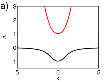
Without the lattice potential, , solutions to the linearized version of Eqs. (1) and (2) are sought for as , which yields the spectrum consisting of two branches,
| (4) |
see Fig. 1(a). The addition of the lattice potential splits this spectrum into multiple bands with the zone folding happening at , see Fig. 1(b). Gaps between the bands are getting wider for deeper lattices (larger ). Unusually, the choice of also affects the gap widths, see Fig. 1(c). This happens because the curvature of the exciton-polariton dispersion without the periodic potential, see Eq. (4), strongly depends on . In contrast, the photonic dispersion is parabolic, and it is modified by the periodic potential in such a way that the width of the primary gap is , being obviously independent of . In Fig. 1(c) we plot the widths of the primary gaps in the two dispersion branches () as functions of . For relatively small , the gaps in the upper and lower polariton branches are approximately the same. Increasing , the dispersion of the upper polariton branch tends to its photonic (light-only) limit, hence the width of the primary gap in the upper branch increases and tends to . For the lower polariton branch, which is the practically important one (see below), first increases and then drops to zero for large , see Fig. 1(c). Below we focus on GSs residing in the principal gap on the lower polariton branch. Our choice of throughout this paper is , which corresponds to modulation period m and matches the experimental conditions of Ref. [10].


III The existence and robustness of gap solitons in the 1D geometry
In order to address the existence of GSs in the model, we first apply the coupled-mode (CM) approximation, which is known to lead to explicit analytical results [13], which are then compared to full numerical solutions of Eqs. (1), (2). To this end, we introduce and assume
| (5) | |||||
where is the frequency as given by Eq. (4) in the middle of the gap, is the polariton eigenvector in the absence of the nonlinearity and periodic potential, and and are slowly varying functions. The substitution of Eq. (5) into Eqs. (1), (2) and manipulations similar to those known in the context of the CM equations for fiber Bragg gratings [13, 23], we derive the CM equations corresponding to the present setting:
| (6) | |||
| (7) |
where is the coefficient of the Bragg-reflection-induced linear coupling between the counterpropagating waves. Figure 1(d) compares the spectra found from the full model and from the CM equations. The good agreement between the two persists for , i.e., for relatively weak potentials.
Using variables and , we obtain from Eqs. (6) and (7) explicit solutions for GSs [13],
| (8) |
| (9) | |||||
| (10) | |||||
| (11) |
where is the frequency detuning relative to the gap center, is the soliton velocity, and .
In Fig. 2 we compare the analytical stationary solitons given by Eqs. (8) and their counterparts found numerically from Eqs. (1) and (2). The overall agreement is reasonable. The main source of the error is the inaccuracy of ratio , which, in the framework of the CM approximation, is taken as per the linear eigenvector at and , therefore it is assumed to remain constant while the soliton’s spectrum is shifting within the gap, following a variation of . However, numerical solutions show a tangible dependence of the ratio on the soliton frequency .


Next, we check the stability of the numerically found GS solutions. To this end, we perturb them by setting , and linearize Eqs. (1), (2) assuming that perturbations and are small. This yields
| (12) | |||||
where . Then, we seek solutions to Eq. (12) as . The existence of eigenvalues with implies instability.
We have found that results of the stability analysis for the full polariton model qualitatively coincide with the known stability properties of the GSs obeying CM equations (6), (7) [22, 23]. In particular, the gap polariton solitons are stable in the lower half of the gap, and feature various instabilities in the upper half, see Fig. 3(a). Figure 3(b) demonstrates that the instability (if any) initiated by random perturbations causes the soliton to ramble erratically across the lattice.


We have also checked numerically mobility and collisions of the GSs in the full model. Figure 4(a) shows a soliton which initially moves through the lattice as prescribed by the CM approximation, but eventually gets pinned around one of the lattice sites. Outcomes of collisions between the solitons are sensitive to both initial velocities and the relative phase of the interacting solitons, as shown in Figs. 4(b)-(d). Collisions between solitons with opposite velocities result in merger of in-phase soliton pairs, and rebound of the solitons with the phase different of , see Figs. 4(b)-(c). Collisions of solitons with different velocities can produce a plethora of outcomes, with one example shown in Fig. 4(c).


IV Gap solitons in the 2D geometry
To examine the relevance of the 1D model elaborated above to the 2D geometry of practical interest, we consider a configuration where the periodic potential acting in the direction is combined with a localized potential applied along the coordinate:
| (18) |
The shape of the above potential is shown in Fig. 5(a). We have found the corresponding 2D soliton solutions numerically, see Fig. 5(b), using a time-independent iteration method.
To check if the dynamics seen in the 1D case is retained in the 2D configuration we have carried out a series of numerical experiments in soliton collisions. The initial conditions were set as
| (19) |
where , and have been chosen to approximate the stationary profile of the numerically found solitons and is the initial soliton momentum. The results of these simulations are shown in Figs. 6 and 7. Similar to the 1D case, the in-phase solitons tend to merge in the course of the collision, while the out-of-phase solitons bounce back. The outcome of the collision of the out-of-phase 2D solitons is similar to what was observed in the 1D model. However, for the in-phase solitons the large-amplitude pattern generated by the merger is, most often, unstable, splitting into two quasi-solitons moving in opposite directions, see Fig. 6. This pair is asymmetric, one of the emerging quasi-solitons being usually larger and slower than the other.


V Summary
We have predicted the existence and studied stability, mobility and interactions of gap polariton solitons in microcavities equipped with periodic photonic potentials. The 1D model has been studied using the CM (coupled-mode) approach, which yields analytical solutions for the solitons, and also by way of the numerical solution of the full system of equations for the photonic and excitonic components of polaritons. Furthermore, we have studied the two-dimensional microcavity with the periodic potential along one dimension and the trapping potential along the other.
B.A.M. appreciates hospitality of the Department of Physics at the University of Bath (UK). A.V.G. and D.V.S. acknowledge support from EPSRC (grant EP/D079225/1).
References
- [1] A. Kavokin, J. J. Baumberg, G. Malpuech, F. P. Laussy, Microcavities (Oxford University Press, 2007).
- [2] A. Baas, J. Ph. Karr, H. Eleuch, E. Giacobino, Phys. Rev. A 69 (2004) 023809.
- [3] N. A. Gippius, S. G. Tikhodeev, V. D. Kulakovskii, D. N. Krizhanovskii, A. I. Tartakovskii, Europhys. Lett. 67 (2004) 997.
- [4] I. Carusotto, C. Ciuti, Phys. Rev. Lett. 93 (2004) 166401.
- [5] P. G. Savvidis, J. J. Baumberg, R. M. Stevenson, M. S. Skolnick, D. M. Whittaker, J. S. Roberts, Phys. Rev. Lett. 84 (2000) 1547.
- [6] A. Amo, D. Sanvitto, F. P. Laussy, D. Ballarini, E. del Valle, M. D. Martin, A. Lemaitre, J. Bloch, D. N. Krizhanovskii, M. S. Skolnick, C. Tejedor, L. Vina, Nature 457 (2009) 291.
- [7] A. M. Kamchatnov, S. A. Darmanyan, M. Neviere, J. of Luminescence 110 (2004) 373.
- [8] A. V. Yulin, O. A. Egorov, F. Lederer, D. V. Skryabin, Phys. Rev. A 78 (2008) 061801.
- [9] O. A. Egorov, D. V. Skryabin, A. V. Yulin, F. Lederer, Phys. Rev. Lett. 102 (2009) 153904.
- [10] C. W. Lai, N. Y. Kim, S. Utsunomiya, G. Roumpos, H. Deng, M.D. Fraser, T. Byrnes, P. Recher, N. Kumada, T. Fujisawa, Y. Yamamoto, Nature 450 (2007) 529.
- [11] K. Cho, K. Okumoto, N. I. Nikolaev, A. L. Ivanov, Phys. Rev. Lett. 94 (2005) 226406 (2005).
- [12] M. M. de Lima, Jr., M. van der Poel, P. V. Santos, J. M. Hvam, Phys. Rev. Lett. 97 (2006) 045501.
- [13] C. M. de Sterke, J. E. Sipe, in: Progress in Optics, vol. 33, edited by E. Wolf (North-Holland:, Amsterdam, 1994), p. 203; Y. S. Kivshar, G. P. Agrawal, Optical Solitons: From Fibers to Photonic Crystals (Academic Press, 2003).
- [14] B. Eiermann, Th. Anker, M. Albiez, M. Taglieber, P. Treutlein, K.-P. Marzlin, M. K. Oberthaler, Phys. Rev. Lett. 92 (2004) 230401.
- [15] B. I. Mantsyzov, Phys. Rev. A 51 (1995) 4939.
- [16] T. Opatrny, B. A. Malomed, G. Kurizki, Phys. Rev. E 60 (1999) 6137.
- [17] E. V. Kazantseva, A. I. Maimistov, Phys. Rev. A 79 (2009) 033812.
- [18] A. Andre and M. D. Lukin, Phys. Rev. Lett. 89 (2002) 143602.
- [19] A. V. Yulin, D. V. Skryabin, P. S. J. Russell, Opt. Express. 13 (2005) 3529; A. G. Vladimirov, D. V. Skryabin, G. Kozyreff, P. Mandel, M. Tlidi, Opt. Express. 14 (2006) 1.
- [20] K. Staliunas, O. Egorov, Y. S. Kivshar, F. Lederer, Phys. Rev. Lett. 101 (2008) 153903.
- [21] A. Zafrany, B. A. Malomed, I. M. Merhasin, Chaos 15 (2005) 037108.
- [22] B. A Malomed and R. S. Tasgal, Phys. Rev. E 49 (1994) 5787; I. V. Barashenkov, D. E. Pelinovsky, E. V. Zemlyanaya, Phys. Rev. Lett. 80 (1998) 5117; A. De Rossi, C. Conti, S. Trillo, Phys. Rev. Lett. 81 (1998) 85.
- [23] A. V. Yulin, D. V. Skryabin, W. J. Firth, Phys. Rev. E 66 (2002) 046603.